Chapter 9: Interferometry and Aperture Synthesis

9.1 Introduction

How can we get higher angular resolution than the simple full width at half maximum of the Airy

function,/D, where D is the largest that we can afford? One answer is indicated in the bottom panel of

Figure 8.18. If we mask off all of our telescope mirror except two small apertures of diameter d at the

edge, the “central peak” of our image becomes twice as sharp as the Airy function but with huge

sidelobes, that is fringes. The figure oversimplifies the situation, since the telescope will still make

superimposed images of diameter /d through each of the apertures, called the primary beam of the

interferometer. If the apertures are separated by a distance D’, the fringe spacing projected up onto the

sky will be /D’, or for convenience if we assume D’ ~ D, /D. Since this angular distance corresponds to

adjacent maxima, the fringe half width at full maximum (or “beam” width) is ~ /2D; that is, we have

doubled the resolution (at the expense of losing a lot of light). In principle, we could try to determine if a

source was resolved by measuring the width of the fringe “peaks”, but it is easier and more quantitative

to base the measurement on the filling-in of the dark fringes as the source becomes larger, the fringe

contrast. We describe this in terms of the visibility:

where Imax and Imin are the maximum and minimum fringe intensities (separated by ~ /2D), respectively.

The structure of a resolved source can be probed by varying the spacing of the apertures and measuring

the visibility as a function of this spacing.

As a thought experiment, one could place pairs of apertures one at a time at all possible distances and

clock angles over the primary mirror of the telescope and use the information (rather painfully) to

reconstruct the image that would have been obtained with the telescope without apertures. At least the

various patterns of fringes should have all the information in that image. This procedure is the basis of

aperture synthesis.

9.2 Radio Interferometry

The Byrd Green Bank Telescope is the largest fully steerable filled-aperture radio telescope, with a size of 100 X 110 meters. The runners up are the Effelsberg telescope, with a diameter of 100 meters, and the Jodrell Bank Lovell Telescope, 76 meters in diameter. The collecting areas of these telescopes are

awesome, but their angular resolutions are poor; at 21 cm wavelength, /D for a 100 meter telescope is about 7 arcmin. These huge structures are difficult to keep in accurate alignment and are subject to huge forces from wind. Proposals for larger telescopes (e.g., the Jodrell Bank Mark IV and V telescopes at 305 and 122 m respectively) pose major engineering challenges for modest improvements in resolution and have also proven to press the limits of what other humans are willing to purchase for astronomers. Other approaches are needed. The Arecibo disk is fixed in the ground and achieves limited ability to point by moving its feed; this concept allows a diameter of 259m. However, the dish must be spherical

and its spherical aberration is corrected near to focus; the operating frequency range extends to 10 GHz, although the ~ 2mm rms surface accuracy results in reduced aperture efficiency at the highest

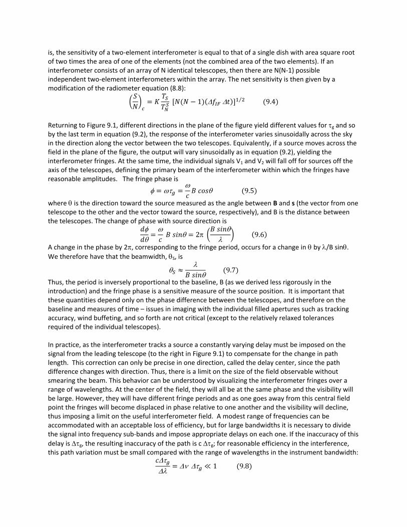
frequencies. The resolution is a bit worse than 2 arcmin (/D) at 21cm. Clearly some other approach is needed to make radio images at resolutions complementary to those in the visible. This approach is to link multiple telescopes through interferometry. Heterodyne receivers provide great flexibility for interferometry because their outputs retain phase information about the incoming signal. Therefore, the functions underlying the interference in the instruments can be conducted off-line. Heterodyne-based interferometers allow implementation of concepts like aperture synthesis, which we explored as a thought experiment in the introduction to this chapter. As a result, very large baselines allow efficient imaging at arcsec or sub-arcsec resolution and large collecting areas can be accumulated by combining the outputs of many telescopes of modest size and cost. 9.2.1 Two-Element Interferometers The basic radio two-element interferometer is shown in Figure 9.1. For simplicity, we assume that the signal is at a single frequency and instant of time so the path difference to the two telescopes can be described by a single phase difference. Since even the most complex combination of multiple radio telescopes can be treated as a large number of two-element interferometers, analyzing the case in Figure 9.1 sets the foundation for the discussion of more advanced telescope arrays used for aperture synthesis. As shown in Figure 9.1, the signals are combined in a cross-correlator, where they are multiplied:

where =2 and RC is the cosine response. The simplification is possible because the terms other than the final one represent multiplication of uncorrelated quantities and hence average to zero. As a result, many potential sources of noise, such as fluctuations in the receiver gains or outside interference, drop out of the signal. The amplitudes V1 and V2 are proportional to the electric field generated from the signal from each telescope, i.e., the gains of the two telescopes. Since the power goes as the autocorrelation of the field, the fields are proportional to the square roots of the telescope areas; therefore, V2 is proportional to the flux density of the source times (A1 A2)1/2, where A1 and A2 are the collecting areas of the two telescopes. Thus, the effective area of the interferometer is

That is, for a two-element interferometer, the effective area is that of one of the elements (assuming they are identical). The noise from the two elements is, however, independent, so the noise in the correlator output is reduced by the square root of two compared with that from a single telescope. That

Figure 9.1. A radio two-element interferometer. After

Garrett.

is, the sensitivity of a two-element interferometer is equal to that of a single dish with area square root of two times the area of one of the elements (not the combined area of the two elements). If an interferometer consists of an array of N identical telescopes, then there are N(N-1) possible independent two-element interferometers within the array. The net sensitivity is then given by a modification of the radiometer equation (8.8):

Returning to Figure 9.1, different directions in the plane of the figure yield different values for g and so by the last term in equation (9.2), the response of the interferometer varies sinusoidally across the sky in the direction along the vector between the two telescopes. Equivalently, if a source moves across the field in the plane of the figure, the output will vary sinusoidally as in equation (9.2), yielding the interferometer fringes. At the same time, the individual signals V1 and V2 will fall off for sources off the axis of the telescopes, defining the primary beam of the interferometer within which the fringes have reasonable amplitudes. The fringe phase is

where is the direction toward the source measured as the angle between B and s (the vector from one telescope to the other and the vector toward the source, respectively), and B is the distance between the telescopes. The change of phase with source direction is

A change in the phase by 2, corresponding to the fringe period, occurs for a change in by /B sin .

We therefore have that the beamwidth, S, is

Thus, the period is inversely proportional to the baseline, B (as we derived less rigorously in the introduction) and the fringe phase is a sensitive measure of the source position. It is important that these quantities depend only on the phase difference between the telescopes, and therefore on the baseline and measures of time – issues in imaging with the individual filled apertures such as tracking accuracy, wind buffeting, and so forth are not critical (except to the relatively relaxed tolerances required of the individual telescopes). In practice, as the interferometer tracks a source a constantly varying delay must be imposed on the signal from the leading telescope (to the right in Figure 9.1) to compensate for the change in path length. This correction can only be precise in one direction, called the delay center, since the path difference changes with direction. Thus, there is a limit on the size of the field observable without smearing the beam. This behavior can be understood by visualizing the interferometer fringes over a range of wavelengths. At the center of the field, they will all be at the same phase and the visibility will be large. However, they will have different fringe periods and as one goes away from this central field point the fringes will become displaced in phase relative to one another and the visibility will decline, thus imposing a limit on the useful interferometer field. A modest range of frequencies can be accommodated with an acceptable loss of efficiency, but for large bandwidths it is necessary to divide the signal into frequency sub-bands and impose appropriate delays on each one. If the inaccuracy of this

delay is g, the resulting inaccuracy of the path is c g; for reasonable efficiency in the interference, this path variation must be small compared with the range of wavelengths in the instrument bandwidth:

From Figure 9.1,

or

where is the angular distance from the delay center. Combining equations (9.6), (9.7), and (9.9), we find the requirement that

to avoid “bandwidth smearing” that broadens the beam in the radial direction. A related requirement is

that the correlator must sample the signals fast enough that the change in beam direction is less than S, or the image will be subject to “time smearing.” In the following, we will ignore these complexities (or assume that the engineering staff has provided sufficient electronics to banish them) and discuss basic interferometer performance. The cosine form in equation (9.2) is sensitive on an extended source only to the symmetric part of the source distribution. The antisymmetric part can be recovered by dividing the output of the telescopes into two signals and applying a 90o phase shift to the signal from one of the telescopes in one of these

pairs. This pair is also cross-correlated to yield an output as in equation (9.2) but with a sin( g) oscillatory component and a sine response analogous to that of equation (9.2).

Correlators with these dual outputs are called complex correlators, because their outputs are generally manipulated as complex numbers combining the amplitude and phase of the signal. The complex visibility is

with the visibility amplitude

and phase

The complex visibility is the response of an interferometer with a complex correlator to an extended source. By the Van Cittert-Zernicke Theorem, the intensity distribution of the source on the sky is the Fourier Transform of the visibility (to be discussed further in Section 9.2.4).

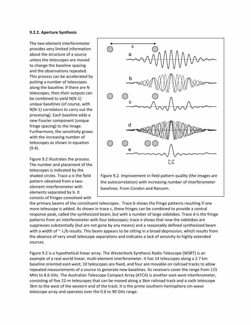
9.2.2. Aperture Synthesis The two-element interferometer provides very limited information about the structure of a source unless the telescopes are moved to change the baseline spacing and the observations repeated. This process can be accelerated by putting a number of telescopes along the baseline; if there are N telescopes, then their outputs can be combined to yield N(N-1) unique baselines (of course, with N(N-1) correlators to carry out the processing). Each baseline adds a new Fourier component (unique fringe spacing) to the image. Furthermore, the sensitivity grows with the increasing number of telescopes as shown in equation (9.4). Figure 9.2 illustrates the process. The number and placement of the telescopes is indicated by the shaded circles. Trace a is the field pattern obtained from a two-element interferometer with elements separated by b. It consists of fringes convolved with the primary beams of the constituent telescopes. Trace b shows the fringe patterns resulting if one more telescope is added. As shown in trace c, these fringes can be combined to provide a central response peak, called the synthesized beam, but with a number of large sidelobes. Trace d is the fringe patterns from an interferometer with four telescopes; trace e shows that now the sidelobes are suppresses substantially (but are not gone by any means) and a reasonably defined synthesized beam

with a width of ~/b results. This beam appears to be sitting in a broad depression, which results from the absence of very small telescope separations and indicates a lack of sensivity to highly extended sources. Figure 9.2 is a hypothetical linear array. The Westerbork Synthesis Radio Telescope (WSRT) is an example of a real-world linear, multi-element interferometer. It has 14 telescopes along a 2.7 km baseline oriented east-west; 10 telescopes are fixed, and four are movable on railroad tracks to allow repeated measurements of a source to generate new baselines. Its receivers cover the range from 115 MHz to 8.6 GHz. The Australian Telescope Compact Array (ATCA) is another east-west interferometer, consisting of five 22-m telescopes that can be moved along a 3km railroad track and a sixth telescope 3km to the west of the western end of the track. It is the prime southern-hemisphere cm-wave telescope array and operates over the 0.6 to 90 GHz range.

Figure 9.2. Improvement in field pattern quality (the images are

the autocorrelation) with increasing number of interferometer

baselines. From Condon and Ransom.

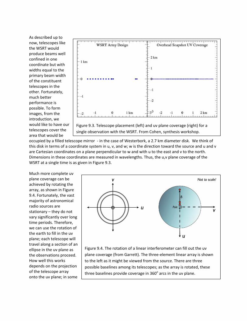
As described up to now, telescopes like the WSRT would produce beams well confined in one coordinate but with widths equal to the primary beam width of the constituent telescopes in the other. Fortunately, much better performance is possible. To form images, from the introduction, we would like to have our telescopes cover the area that would be occupied by a filled telescope mirror - in the case of Westerbork, a 2.7 km diameter disk. We think of this disk in terms of a coordinate system in u, v, and w; w is the direction toward the source and u and v are Cartesian coordinates on a plane perpendicular to w and with u to the east and v to the north. Dimensions in these coordinates are measured in wavelengths. Thus, the u,v plane coverage of the WSRT at a single time is as given in Figure 9.3. Much more complete uv plane coverage can be achieved by rotating the array, as shown in Figure 9.4. Fortunately, the vast majority of astronomical radio sources are stationary – they do not vary significantly over long time periods. Therefore, we can use the rotation of the earth to fill in the uv plane; each telescope will travel along a section of an ellipse in the uv plane as the observations proceed. How well this works depends on the projection of the telescope array onto the uv plane; in some

Figure 9.3. Telescope placement (left) and uv plane coverage (right) for a

single observation with the WSRT. From Cohen, synthesis workshop.

Figure 9.4. The rotation of a linear interferometer can fill out the uv

plane coverage (from Garrett). The three-element linear array is shown

to the left as it might be viewed from the source. There are three

possible baselines among its telescopes; as the array is rotated, these

three baselines provide coverage in 360o arcs in the uv plane.

directions, e.g., at the celestial equator, the ellipses may be significantly foreshortened (for a linear E-W array like Westerbork). The situation for the WSRT is summarized in Figure 9.5, and the foreshortening is illustrated in Figure 9.6.

Figure 9.5. uv plane coverage with Westerbork for full synthesis. The latitude of the telescope is

approximately 53o, accounting for the excellent coverage at a declination of 60o. At the celesctial

equator, the rotation of the earth does not change the array orientation in celestial coordinates.

Other declinations are intermediate in behavior. From Cohen.

Figure 9.6. The uv plane coverage (left) of a two-element

interferometer at 40o latitude, for a radio source at +30o

declination, from Condon and Ransom. The right panel shows

how foreshortening of the array is responsible for the less

extensive coverage in the v direction.

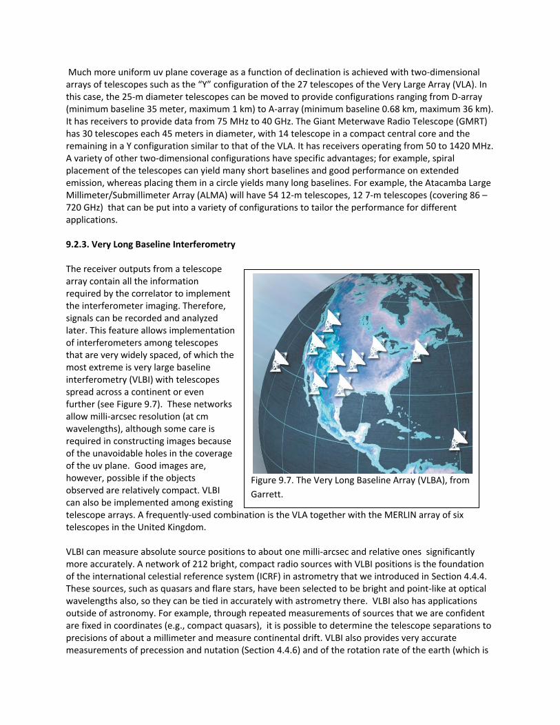
Much more uniform uv plane coverage as a function of declination is achieved with two-dimensional arrays of telescopes such as the “Y” configuration of the 27 telescopes of the Very Large Array (VLA). In this case, the 25-m diameter telescopes can be moved to provide configurations ranging from D-array (minimum baseline 35 meter, maximum 1 km) to A-array (minimum baseline 0.68 km, maximum 36 km). It has receivers to provide data from 75 MHz to 40 GHz. The Giant Meterwave Radio Telescope (GMRT) has 30 telescopes each 45 meters in diameter, with 14 telescope in a compact central core and the remaining in a Y configuration similar to that of the VLA. It has receivers operating from 50 to 1420 MHz. A variety of other two-dimensional configurations have specific advantages; for example, spiral placement of the telescopes can yield many short baselines and good performance on extended emission, whereas placing them in a circle yields many long baselines. For example, the Atacamba Large Millimeter/Submillimeter Array (ALMA) will have 54 12-m telescopes, 12 7-m telescopes (covering 86 – 720 GHz) that can be put into a variety of configurations to tailor the performance for different applications. 9.2.3. Very Long Baseline Interferometry The receiver outputs from a telescope array contain all the information required by the correlator to implement the interferometer imaging. Therefore, signals can be recorded and analyzed later. This feature allows implementation of interferometers among telescopes that are very widely spaced, of which the most extreme is very large baseline interferometry (VLBI) with telescopes spread across a continent or even further (see Figure 9.7). These networks allow milli-arcsec resolution (at cm wavelengths), although some care is required in constructing images because of the unavoidable holes in the coverage of the uv plane. Good images are, however, possible if the objects observed are relatively compact. VLBI can also be implemented among existing telescope arrays. A frequently-used combination is the VLA together with the MERLIN array of six telescopes in the United Kingdom. VLBI can measure absolute source positions to about one milli-arcsec and relative ones significantly more accurately. A network of 212 bright, compact radio sources with VLBI positions is the foundation of the international celestial reference system (ICRF) in astrometry that we introduced in Section 4.4.4. These sources, such as quasars and flare stars, have been selected to be bright and point-like at optical wavelengths also, so they can be tied in accurately with astrometry there. VLBI also has applications outside of astronomy. For example, through repeated measurements of sources that we are confident are fixed in coordinates (e.g., compact quasars), it is possible to determine the telescope separations to precisions of about a millimeter and measure continental drift. VLBI also provides very accurate measurements of precession and nutation (Section 4.4.6) and of the rotation rate of the earth (which is

Figure 9.7. The Very Long Baseline Array (VLBA), from

Garrett.

slowing). Accurate time keeping requires reconciliation of the length of the day with coordinated universal time (UTC) and the occasional slight adjustments (“leap seconds”) are determined from VLBI. Equation (9.3) was discussed in terms of two telescope of equal diameter, but it holds in general. As a result, there are interesting options for VLBI using a modest-sized telescope in orbit or even on the moon to provide a huge baseline. If a very large groundbased telescope is used, the effective area can be reasonably large and hence good sensitivity can be obtained. 9.2.4. Interpretation of Aperture Synthesis Data Ideally, we would use our telescope array (and the rotation of the earth) to measure visibilities for our source densely spaced over the entire uv plane. The Fourier transform of this visibility function V(uv) would give us an image of the target source just as if it had been observed with a filled aperture telescope with diameter equal to the diameter of our telescope array:

(by the Van Cittert-Zernicky Theorem). However, realistic telescope arrays and observing strategies will leave gaps in the uv plane coverage, and as a result we have a “dirty” image:

where S(u,v) is the sampling function over the uv plane, 1 where we have a measurement and 0 otherwise. Consequently, our point spread function will have more artifacts than would have been the case in the ideal case. From the form of equation (9.15) and the convolution theorem, our image is

the true distribution convolved with our point spread function, which may depart significantly from the ideal if S(u,v) is sparse. B(x,y) is termed the dirty beam :

See Figure 9.8 for an example of a dirty beam. Even if our target area is the simple case of a field of unresolved sources, the superposition of the dirty beams for all of them will leave our image looking like a bit of a mess, as in Figure 9.9. The simplest approach to converting data such as in Figure 9.9 into something suitable to show off to others is the Hogbom CLEAN algorithm. To implement it, one: 1.) assumes that the image can be approximated by a field of point sources; 2.) Locates the position of the brightest point in the dirty map; 3.) subtracts a scaled version of the dirty beam from this position; the subtraction should account for only a modest fraction of the brightness at this point; 4.) Records the position and subtracted intensity in a “CLEAN component” file; 5.) Finds the brightest position in the dirty map left from the subtraction;

Figure 9.8. A Dirty Beam, from Garrett

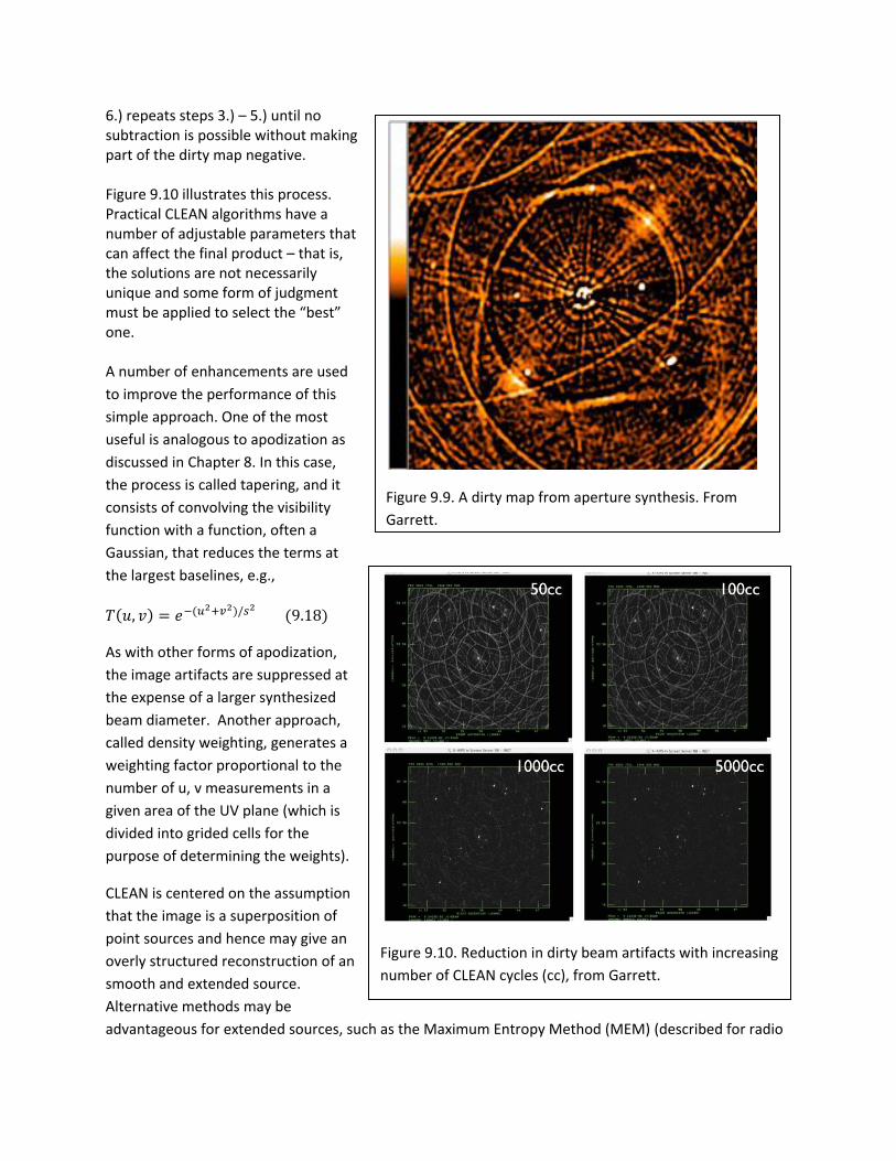
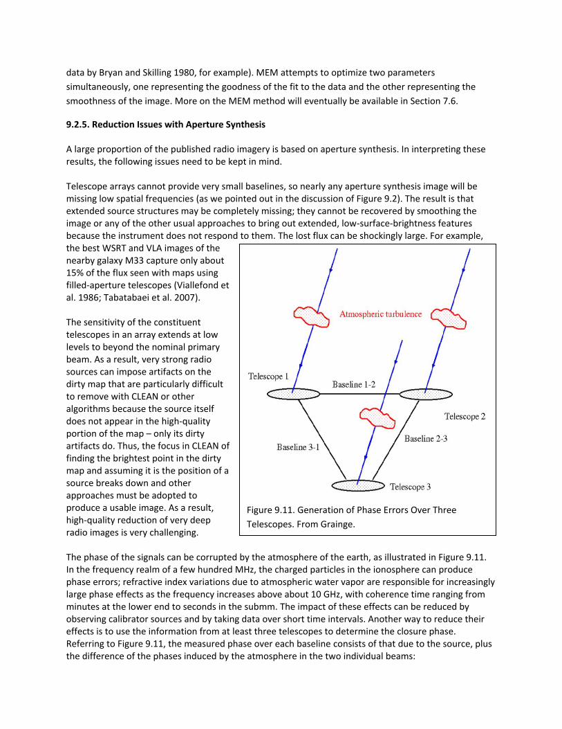
6.) repeats steps 3.) – 5.) until no subtraction is possible without making part of the dirty map negative. Figure 9.10 illustrates this process. Practical CLEAN algorithms have a number of adjustable parameters that can affect the final product – that is, the solutions are not necessarily unique and some form of judgment must be applied to select the “best” one. A number of enhancements are used

to improve the performance of this

simple approach. One of the most

useful is analogous to apodization as

discussed in Chapter 8. In this case,

the process is called tapering, and it

consists of convolving the visibility

function with a function, often a

Gaussian, that reduces the terms at

the largest baselines, e.g.,

As with other forms of apodization,

the image artifacts are suppressed at

the expense of a larger synthesized

beam diameter. Another approach,

called density weighting, generates a

weighting factor proportional to the

number of u, v measurements in a

given area of the UV plane (which is

divided into grided cells for the

purpose of determining the weights).

CLEAN is centered on the assumption

that the image is a superposition of

point sources and hence may give an

overly structured reconstruction of an

smooth and extended source.

Alternative methods may be

advantageous for extended sources, such as the Maximum Entropy Method (MEM) (described for radio

Figure 9.10. Reduction in dirty beam artifacts with increasing

number of CLEAN cycles (cc), from Garrett.

Figure 9.9. A dirty map from aperture synthesis. From

Garrett.

data by Bryan and Skilling 1980, for example). MEM attempts to optimize two parameters

simultaneously, one representing the goodness of the fit to the data and the other representing the

smoothness of the image. More on the MEM method will eventually be available in Section 7.6.

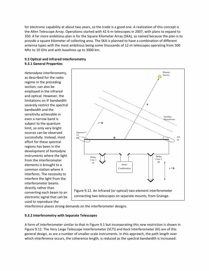
9.2.5. Reduction Issues with Aperture Synthesis A large proportion of the published radio imagery is based on aperture synthesis. In interpreting these results, the following issues need to be kept in mind. Telescope arrays cannot provide very small baselines, so nearly any aperture synthesis image will be missing low spatial frequencies (as we pointed out in the discussion of Figure 9.2). The result is that extended source structures may be completely missing; they cannot be recovered by smoothing the image or any of the other usual approaches to bring out extended, low-surface-brightness features because the instrument does not respond to them. The lost flux can be shockingly large. For example, the best WSRT and VLA images of the nearby galaxy M33 capture only about 15% of the flux seen with maps using filled-aperture telescopes (Viallefond et al. 1986; Tabatabaei et al. 2007). The sensitivity of the constituent telescopes in an array extends at low levels to beyond the nominal primary beam. As a result, very strong radio sources can impose artifacts on the dirty map that are particularly difficult to remove with CLEAN or other algorithms because the source itself does not appear in the high-quality portion of the map – only its dirty artifacts do. Thus, the focus in CLEAN of finding the brightest point in the dirty map and assuming it is the position of a source breaks down and other approaches must be adopted to produce a usable image. As a result, high-quality reduction of very deep radio images is very challenging. The phase of the signals can be corrupted by the atmosphere of the earth, as illustrated in Figure 9.11. In the frequency realm of a few hundred MHz, the charged particles in the ionosphere can produce phase errors; refractive index variations due to atmospheric water vapor are responsible for increasingly large phase effects as the frequency increases above about 10 GHz, with coherence time ranging from minutes at the lower end to seconds in the submm. The impact of these effects can be reduced by observing calibrator sources and by taking data over short time intervals. Another way to reduce their effects is to use the information from at least three telescopes to determine the closure phase. Referring to Figure 9.11, the measured phase over each baseline consists of that due to the source, plus the difference of the phases induced by the atmosphere in the two individual beams:

Figure 9.11. Generation of Phase Errors Over Three

Telescopes. From Grainge.

(9.20)

The sum of equations (9.19) – (9.21) is

In this closure phase the atmospheric-induced phase errors have all canceled. With four telescopes, it is possible to deduce a quantity analogous to the closure phase for the signal amplitudes. By modeling the closure phases and amplitude information in a telescope array, it is possible to deduce the source structure independent of the phase errors. These procedures are most effective on relatively bright sources, so that there is enough signal in a coherence time that the atmospheric effects are stationary. Another approach is called self-calibration. It requires that there is a point source in the primary beam that is bright enough to be detected in all the interferometer baselines within a coherence time. If so, then one can use a beginning model of the source, compute its visibilities and subtract from the observed ones, use CLEAN on the residuals to deduce the implied correction in the model, and repeat the comparison. This iteration is repeated until it converges, as indicated when the corrections are no longer significant. 9.2.6 The Future The VLA has been the flagship aperture synthesis array for cm-wave radio astronomy since its commissioning. The current transmission of signals from the VLA receivers to the correlators has limited IF bandwidth, a problem that is being solved by installation of optical fiber links between the telescopes. Similar upgrades have been made in MERLIN and the European VLBI network. These links will enable bandwidths of ~ 2 GHz, improving the achievable signal to noise by factors of 5-10 (equation 9.4). The broader frequency/wavelength coverage can also substantially improve the coverage of the uv plane; since u and v are measured in wavelength units, a given physical baseline corresponds to a range of positions in uv if the range of wavelengths is significant. We have already mentioned ALMA in the context of telescope configurations for interferometers. This array of 54 12-m telescopes and 12 7-m ones is placed at an altitude of about 5000 meters on the Chajnantor plateau in Chile, above the great majority of the atmospheric water vapor. (Recall from Section 1.4.2 that the scale height for water vapor in the atmosphere is about 2km, so there is only about 8% of the nominal sea-level value at the ALMA altitude). The dramatic reduction in the water vapor over ALMA both enhances the atmospheric transparency in the submm substantially and reduces the phase errors. ALMA incorporates state-of-the art sideband-separating receivers and broadband IF links for very high sensitivity over a range of 86 to 720 GHz. The telescopes can be moved into a variety of configurations to optimize ALMA for specific types of observation. ALMA will begin operation soon with some of its telescopes. Our discussion of the limitations to the sizes of filled-aperture radio telescopes, plus equation 9.4 and the discussion surrounding it, suggests a new approach to very large collecting areas. One could build a huge number of modest sized telescopes (thus providing large primary beams, making imaging and mapping efficient) into an aperture synthesis interferometer. Since the number of correlators grows as the number of baselines, e.g. as N(N-1) for N telescopes, one is trading mechanical challenges for electronic ones. Judging by the growth of optical telescopes over the last century, the doubling time for telescope diameters is about 30 years, whereas the well-known Moore’s Law places the doubling time

for electronic capability at about two years, so the trade is a good one. A realization of this concept is the Allen Telescope Array. Operations started with 42 6-m telescopes in 2007, with plans to expand to 350. A far more ambitious plan is for the Square Kilometer Array (SKA), so named because the plan is to provide a square kilometer of collecting area. The SKA is planned to have a combination of different antenna types with the most ambitious being some thousands of 12-m telescopes operating from 500 Mhz to 10 GHz and with baselines up to 3000 km. 9.3 Optical and Infrared Interferometry 9.3.1 General Properties Heterodyne interferometry, as described for the radio regime in the preceding section, can also be employed in the infrared and optical. However, the limitations on IF bandwidth severely restrict the spectral bandwidth and the sensitivity achievable in even a narrow band is subject to the quantum limit, so only very bright sources can be observed successfully. Instead, most effort for these spectral regions has been in the development of homodyne instruments where the light from the interferometer elements is brought to a common station where it interferes. The necessity to interfere the light from the interferometer beams directly rather than converting each beam to an electronic signal that can be used to reproduce the interference places strong demands on the interferometer designs. 9.3.2 Interferometry with Separate Telescopes A form of interferometer similar to that in Figure 9.1 but incorporating this new restriction is shown in Figure 9.12. The Very Large Telescope Interferometer (VLTI) and Keck Interferometer (KI) are of this general design, as are a number of smaller-scale instruments. In this approach, the path length over which interference occurs, the coherence length, is reduced as the spectral bandwidth is increased:

Figure 9.12. An Infrared (or optical) two-element interferometer

connecting two telescopes on separate mounts, from Grainge.

An optical train or “delay line” with precision moving elements is used to make the path length correction to this level of accuracy. It is too complex to try to correct the path difference to this accuracy over a significant field of view. Therefore, the usable field is very small,

In addition, the correcting optics are in air, so the dispersion of air (equation (7.1)) results in different path length corrections for different wavelengths, or more practically, places a restriction on the spectral band that can be observed for a single correction. For example, for a 100m baseline, a spectral

resolution of / ~ 12 is the maximum allowable at J band (1.25 m) to get good fringe visibilities.

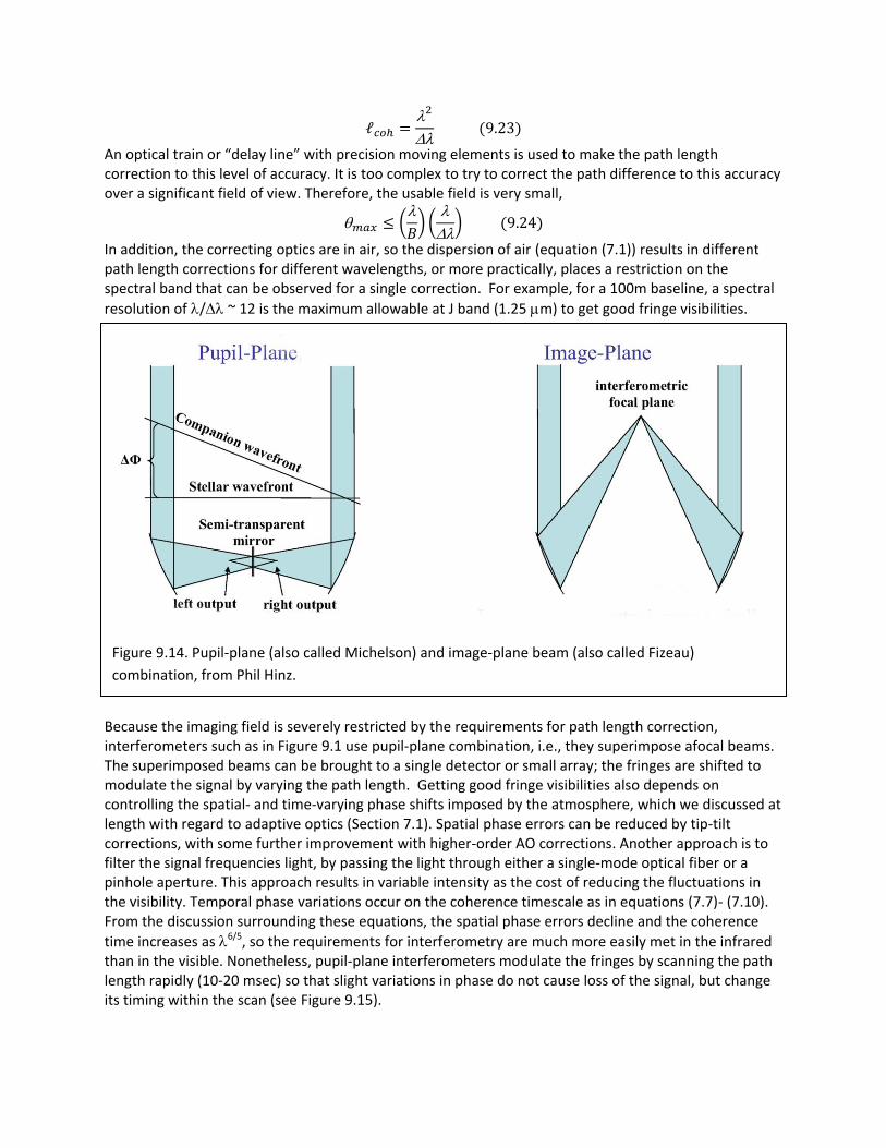
Because the imaging field is severely restricted by the requirements for path length correction, interferometers such as in Figure 9.1 use pupil-plane combination, i.e., they superimpose afocal beams. The superimposed beams can be brought to a single detector or small array; the fringes are shifted to modulate the signal by varying the path length. Getting good fringe visibilities also depends on controlling the spatial- and time-varying phase shifts imposed by the atmosphere, which we discussed at length with regard to adaptive optics (Section 7.1). Spatial phase errors can be reduced by tip-tilt corrections, with some further improvement with higher-order AO corrections. Another approach is to filter the signal frequencies light, by passing the light through either a single-mode optical fiber or a pinhole aperture. This approach results in variable intensity as the cost of reducing the fluctuations in the visibility. Temporal phase variations occur on the coherence timescale as in equations (7.7)- (7.10). From the discussion surrounding these equations, the spatial phase errors decline and the coherence

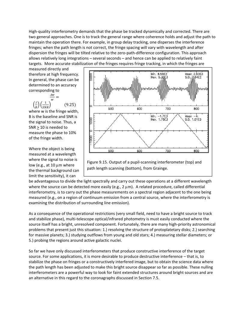
time increases as 6/5, so the requirements for interferometry are much more easily met in the infrared than in the visible. Nonetheless, pupil-plane interferometers modulate the fringes by scanning the path length rapidly (10-20 msec) so that slight variations in phase do not cause loss of the signal, but change its timing within the scan (see Figure 9.15).

Figure 9.14. Pupil-plane (also called Michelson) and image-plane beam (also called Fizeau)

combination, from Phil Hinz.

High-quality interferometry demands that the phase be tracked dynamically and corrected. There are two general approaches. One is to track the general range where coherence holds and adjust the path to maintain the operation there. For example, in group delay tracking, one disperses the interference fringes; when the path length is not correct, the fringe spacing will vary with wavelength and after dispersion the fringes will be tilted relative to the zero-path-difference configuration. This approach allows relatively long integrations – several seconds – and hence can be applied to relatively faint targets. More accurate stabilization of the fringes requires fringe tracking, in which the fringes are measured directly and therefore at high frequency. In general, the phase can be determined to an accuracy corresponding to

where w is the fringe width, B is the baseline and SNR is the signal to noise. Thus, a SNR > 10 is needed to measure the phase to 10% of the fringe width. Where the object is being measured at a wavelength where the signal to noise is

low (e.g., at 10 m where the thermal background can limit the sensitivity), it can be advantageous to divide the light spectrally and carry out these operations at a different wavelength

where the source can be detected more easily (e.g., 2 m). A related procedure, called differential interferometry, is to carry out the phase measurements on a spectral region adjacent to the one being measured (e.g., on a region of continuum emission from a central source, where the interferometry is examining the distribution of surrounding line emission). As a consequence of the operational restrictions (very small field, need to have a bright source to track and stabilize phase), multi-telescope optical/infrared photometry is must easily conducted where the source itself has a bright, unresolved component. Fortunately, there are many high-priority astronomical problems that present just this situation: 1.) resolving the structure of protoplatetary disks; 2.) searching for massive planets; 3.) studying outflows from young and old stars; 4.) measuring stellar diameters; or 5.) probing the regions around active galactic nuclei. So far we have only discussed interferometers that produce constructive interference of the target source. For some applications, it is more desirable to produce destructive interference – that is, to stabilize the phase on fringes or a constructively interfered image, but to obtain the science data where the path length has been adjusted to make this bright source disappear so far as possible. These nulling interferometers are a powerful way to look for faint extended structures around bright sources and are an alternative in this regard to the coronagraphs discussed in Section 7.5.

Figure 9.15. Output of a pupil-scanning interferometer (top) and

path length scanning (bottom), from Grainge.

9.3.3. Common-Mount Interferometry An alternative approach to Figure 9.1 is to use two telescopes on a common mount, arranged so they track a target nominally with no path length difference between their outputs. The true path length difference is then relatively small, so no elaborate delay lines are required to make the necessary adjustments to achieve interference. Of course, to achieve interference, a modest pathlength adjustment is required, and it must be controlled to compensate for the atmospheric phase variations (fast) and flexure in the telescope (slow). The price of this arrangement is that long baselines are not feasible. However, there is potentially another major advantage – such instruments can provide reasonably large fields of view with image diameters corresponding to the interferometer baseline. To provide an imaging field, the interferometer must obey the sine condition requiring that the image plane have the same geometry as the object plane. That is, the relation of the telescopes as viewed from the source must be preserved optically when their outputs are superimposed to cause them to interfere. Preserving the sine condition is virtually impossible with telescopes on separate mounts, hence their small fields of view. However, since placing the two telescopes on the same mount can relieve the issues associated with delay lines, this optical requirement can be met straightforwardly. The outputs of the telescopes need to be brought together with this geometry at an image plane (right side of Figure 9.14). There, the image of a point source will be the Fourier Transform of the entrance aperture(s), and will not vary substantially over the field of the instrument. The image of a spatially resolved object is then the convolution of its spatial distribution of flux with this point spread function. Common-mount interferometers must also satisfy the requirements for phase stability. Because they are imaging instruments, a full AO correction is desirable to provide constant spatial phase over their fields of view. Fringe tracking requires measuring the fringe position in the imaging plane and stabilizing it by feeding back a correction into the pathlength compensator. With separate- and common-mount interferometers, earth rotation is used to fill in the uv plane and probe the structure of a source in two dimensions on the sky, just as discussed for radio interferometers. References Hogbom 1974, A&A Suppl., 15, 417 Tabatabaei, F. S., Krause, M., & Beck, R. 2007, A&A, 472, 785 Viallefond, F., Goss, W. M., van der Hulst, J. M., & Crane, P. C. 1986, A&AS, 64, 237 Further Reading Burke, B. F., and Graham-Smith, F. 2009, “Introduction to Radio Astronomy,” 3rd ed., Cambridge University Press. Condon, J. J., and Ransom, S. M. 2010, “Essential Radio Astronomy,” http://www.cv.nrao.edu/course/astr534/ERA.shtml Kellermann, K. I., and Moran, J. M. 2001, ARAA, 39, 457 Monnier, J. D. 2003, “Optical Interferometry in Astronomy,” Rep Prog. Phys., 66, 789