Chapter 9 Input Modeling Banks, Carson, Nelson & Nicol Discrete-Event System Simulation.
42
Chapter 9 Input Modeling Banks, Carson, Nelson & Nicol Discrete-Event System Simulation
-
Upload
winfred-francis-reeves -
Category
Documents
-
view
383 -
download
40
Transcript of Chapter 9 Input Modeling Banks, Carson, Nelson & Nicol Discrete-Event System Simulation.
Chapter 9 Input Modeling
Banks, Carson, Nelson & Nicol
Discrete-Event System Simulation
2
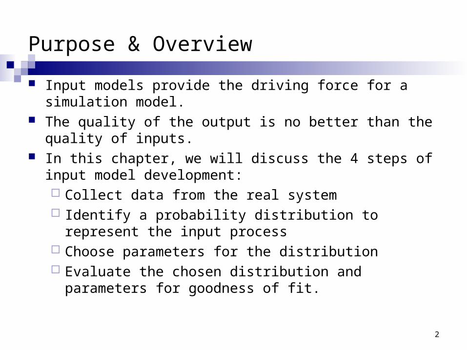
Purpose & Overview
Input models provide the driving force for a simulation model. The quality of the output is no better than the quality of inputs. In this chapter, we will discuss the 4 steps of input model
development: Collect data from the real system Identify a probability distribution to represent the input
process Choose parameters for the distribution Evaluate the chosen distribution and parameters for
goodness of fit.
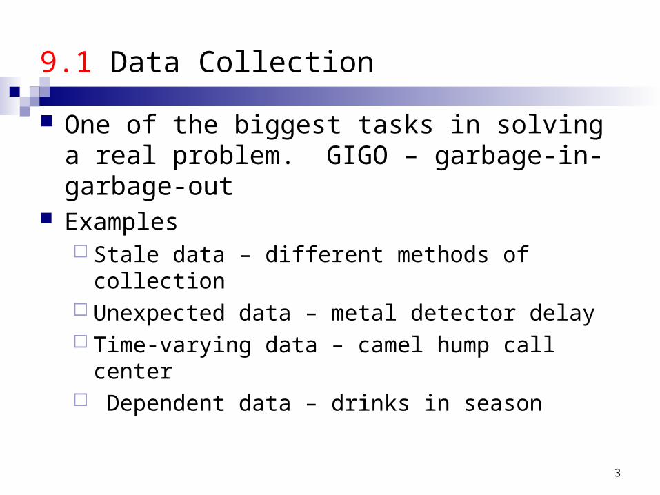
9.1 Data Collection
One of the biggest tasks in solving a real problem. GIGO – garbage-in-garbage-out
Examples Stale data – different methods of collection Unexpected data – metal detector delay Time-varying data – camel hump call center Dependent data – drinks in season
3
4
Data Collection - suggestions start on page 340
Suggestions that may enhance and facilitate data collection: Plan ahead: begin by a practice or pre-observing session, watch
for unusual circumstances Analyze the data as it is being collected: check adequacy Combine homogeneous data sets, e.g. successive time periods,
during the same time period on successive days Be aware of data censoring: the quantity is not observed in its
entirety, danger of leaving out long process times Check for relationship between variables, e.g. build scatter
diagram Check for autocorrelation Collect input data, not performance data
5
9.2 Identifying the Distribution
Histograms Selecting families of distribution Parameter estimation Goodness-of-fit tests Fitting a non-stationary process
6
Histograms [Identifying the distribution]
A frequency distribution or histogram is useful in determining the shape of a distribution
1. Divide the range of data into intervals. (Usually of equal length)
2. Label the horizontal axis to conform to the intervals selected.
3. Find the frequency of occurrences within each interval.4. Label the vertical axis so that the total occurrences
can be plotted for each interval.5. Plot the frequencies on the vertical axis.

Histograms continued
The number of class intervals depends on: The number of observations The dispersion of the data Suggested: the square root of the sample size
For continuous data: Corresponds to the probability density function of a theoretical
distribution For discrete data:
Corresponds to the probability mass function If few data points are available: combine adjacent cells to
eliminate the ragged appearance of the histogram Does this differ from homogeneity in Section 9.1?
7
8
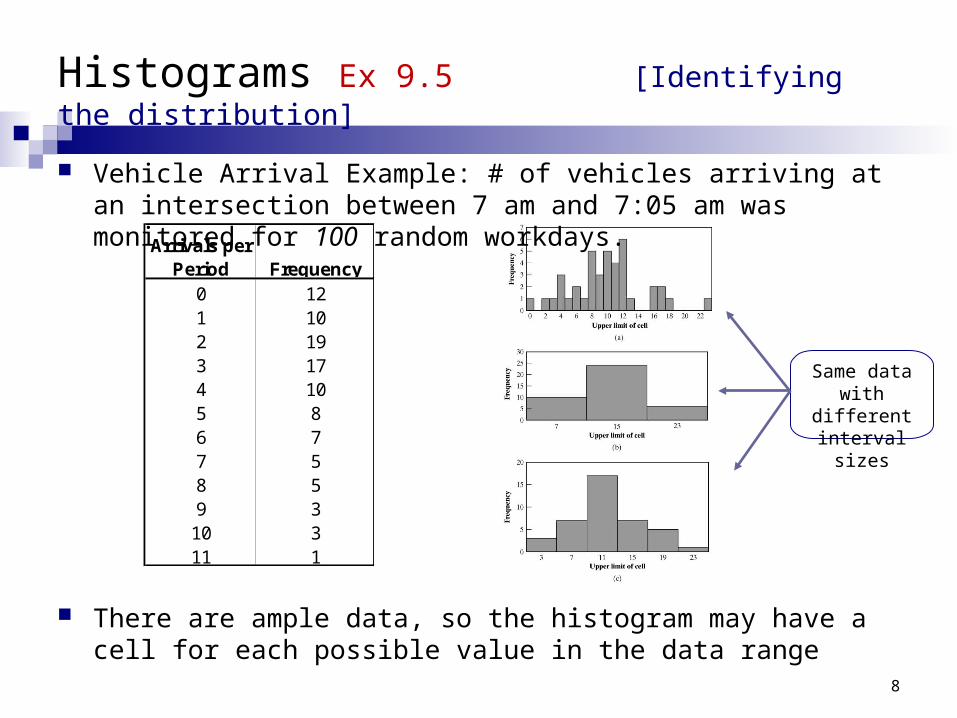
Histograms Ex 9.5 [Identifying the distribution]
Vehicle Arrival Example: # of vehicles arriving at an intersection between 7 am and 7:05 am was monitored for 100 random workdays.
There are ample data, so the histogram may have a cell for each possible value in the data range
Arrivals per Period Frequency
0 121 102 193 174 105 86 77 58 59 310 311 1
Same data with different interval sizes
9
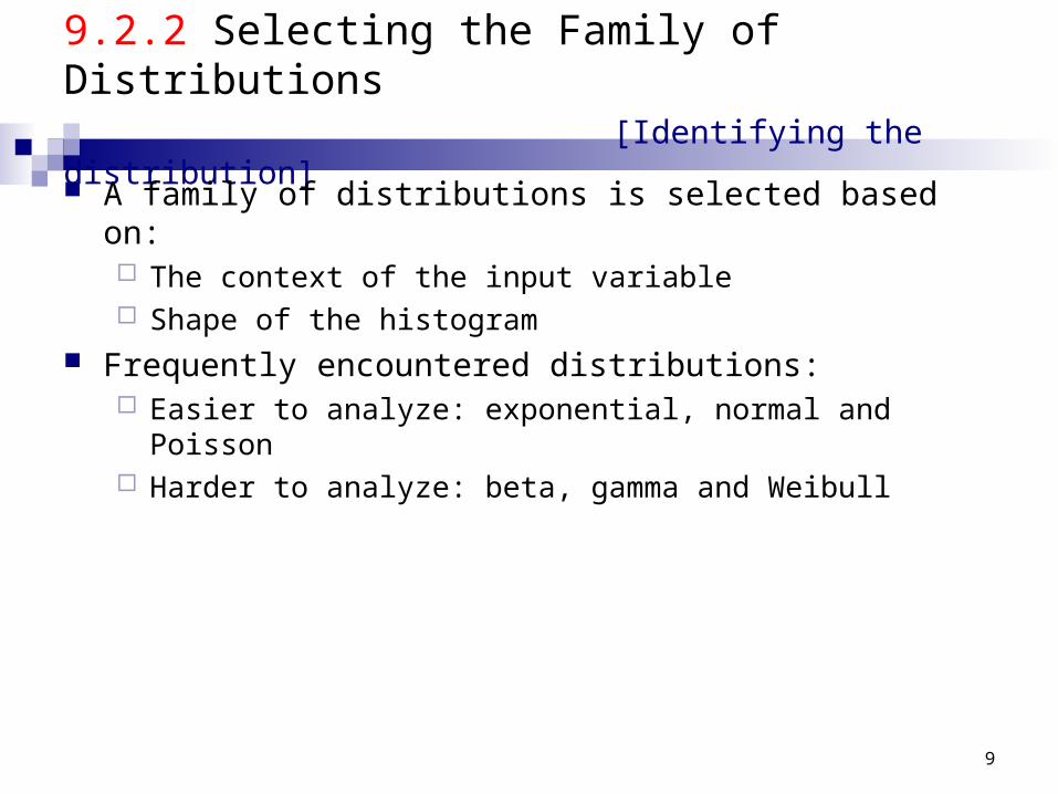
9.2.2 Selecting the Family of Distributions [Identifying the distribution]
A family of distributions is selected based on: The context of the input variable Shape of the histogram
Frequently encountered distributions: Easier to analyze: exponential, normal and Poisson Harder to analyze: beta, gamma and Weibull

10
Selecting the Family of Distributions [Identifying the distribution]
Page 346: Use the physical basis of the distribution as a guide, for example: Binomial: # of successes in n trials Poisson: # of independent events that occur in a fixed amount of
time or space Normal: dist’n of a process that is the sum of a number of
component processes Exponential: time between independent events, or a process time
that is memoryless Weibull: time to failure for components Discrete or continuous uniform: models complete uncertainty Triangular: a process for which only the minimum, most likely,
and maximum values are known Empirical: resamples from the actual data collected
11
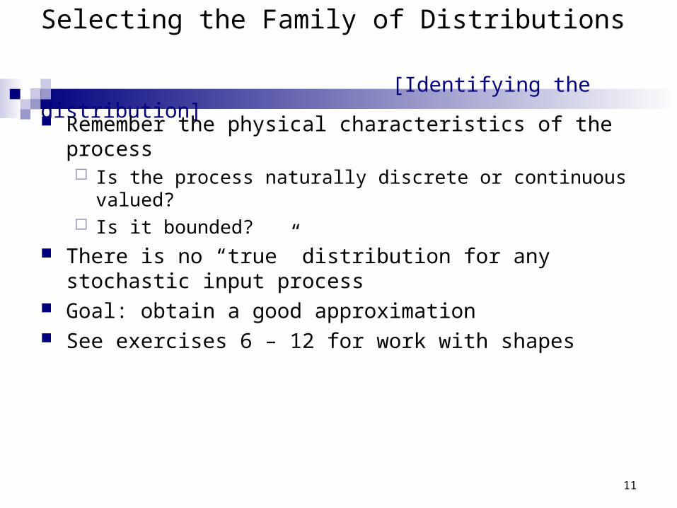
Selecting the Family of Distributions [Identifying the distribution]
Remember the physical characteristics of the process Is the process naturally discrete or continuous valued? Is it bounded?
There is no “true” distribution for any stochastic input process Goal: obtain a good approximation See exercises 6 – 12 for work with shapes

12
Quantile-Quantile Plots [Identifying the distribution]
Q-Q plot is a useful tool for evaluating the fit of the chosen distribution
If X is a random variable with cdf F, then the q-quantile of X is the such that
When F has an inverse, = F-1(q)
Let {xi, i = 1,2, …., n} be a sample of data from X and {yj, j = 1,2, …, n} be the observations in ascending order:
where j is the ranking or order number
, for 0 1F( ) P(X ) q q
1 0.5is approximately -
j
j -y F
n
13
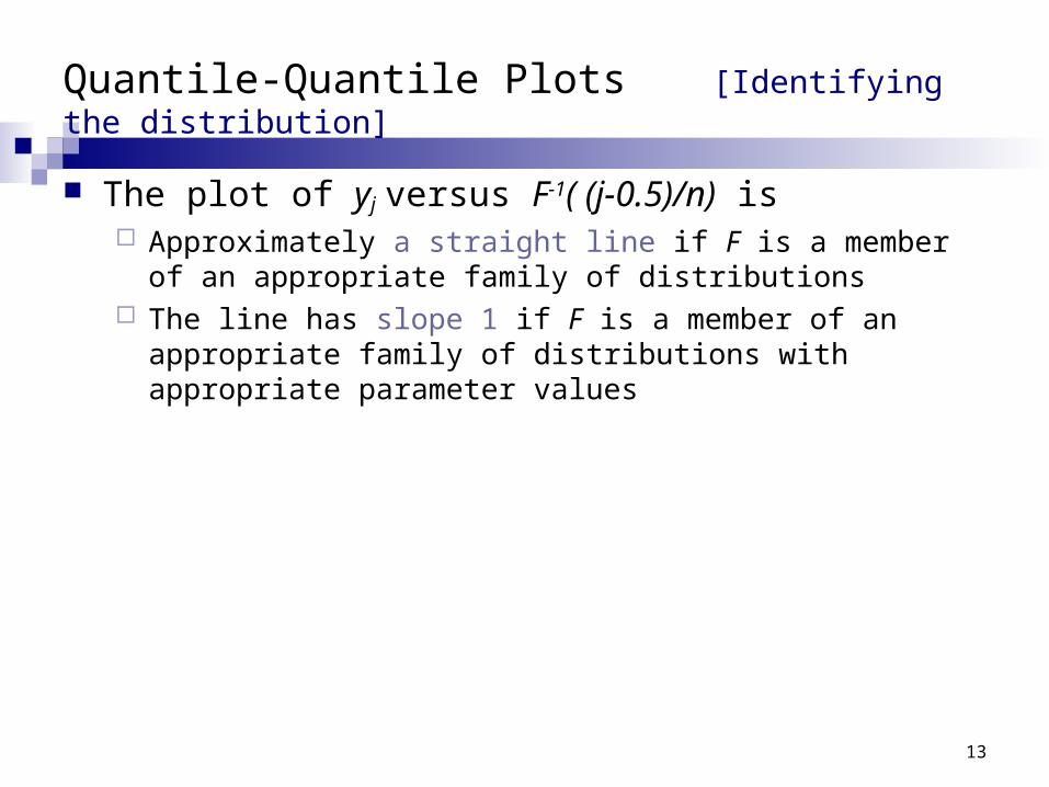
Quantile-Quantile Plots [Identifying the distribution]
The plot of yj versus F-1( (j-0.5)/n) is Approximately a straight line if F is a member of an appropriate
family of distributions The line has slope 1 if F is a member of an appropriate family of
distributions with appropriate parameter values
14
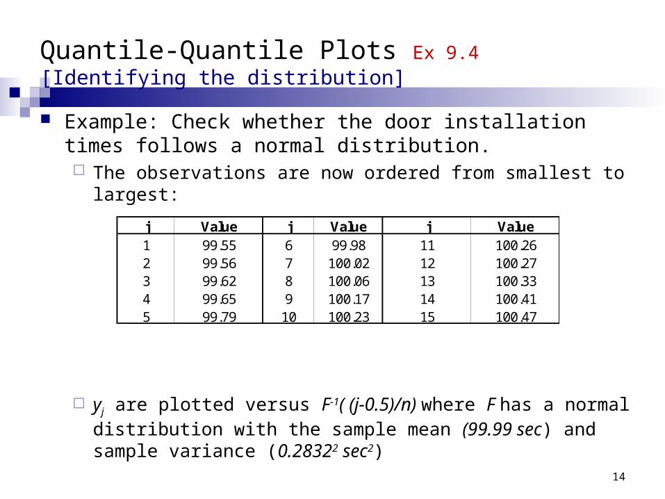
Quantile-Quantile Plots Ex 9.4 [Identifying the distribution]
Example: Check whether the door installation times follows a normal distribution. The observations are now ordered from smallest to largest:
yj are plotted versus F-1( (j-0.5)/n) where F has a normal distribution with the sample mean (99.99 sec) and sample variance (0.28322 sec2)
j Value j Value j Value1 99.55 6 99.98 11 100.262 99.56 7 100.02 12 100.273 99.62 8 100.06 13 100.334 99.65 9 100.17 14 100.415 99.79 10 100.23 15 100.47
15
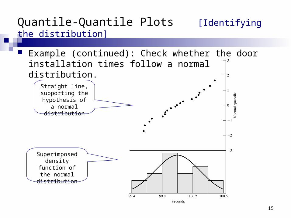
Quantile-Quantile Plots [Identifying the distribution]
Example (continued): Check whether the door installation times follow a normal distribution.
Straight line, supporting the hypothesis of a
normal distribution
Superimposed density function of
the normal distribution
16
Quantile-Quantile Plots [Identifying the distribution]
Consider the following while evaluating the linearity of a q-q plot: The observed values never fall exactly on a straight line The ordered values are ranked and hence not independent,
unlikely for the points to be scattered about the line Variance of the extremes is higher than the middle. Linearity of
the points in the middle of the plot is more important. Q-Q plot can also be used to check homogeneity
Check whether a single distribution can represent both sample sets
Plotting the order values of the two data samples against each other
17
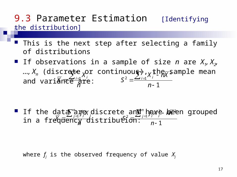
9.3 Parameter Estimation [Identifying the distribution]
This is the next step after selecting a family of distributions If observations in a sample of size n are X1, X2, …, Xn (discrete
or continuous), the sample mean and variance are:
If the data are discrete and have been grouped in a frequency distribution:
where fj is the observed frequency of value Xj
1 1
2221
n
XnXS
n
XX
n
i i
n
i i
1 1
22
21
n
XnXfS
n
XfX
n
j jj
n
j jj

18
Grouped data – example 9.8 on page 350 [Parameter estimation - Identifying the distribution]
Vehicle Arrival Example (continued): Table in the histogram example on slide 6 (Table 9.1 in book) can be analyzed to obtain:
The sample mean and variance are
The histogram suggests X to have a Possion distribution However, note that sample mean is not equal to sample variance. Reason: each estimator is a random variable, is not perfect.
k
j jj
k
j jj XfXf
XfXfn
1
2
1
2211
2080 and ,364 and
,...,1,10,0,12,100
63.799
)64.3(*1002080
3.64100
364
22
S
X
19
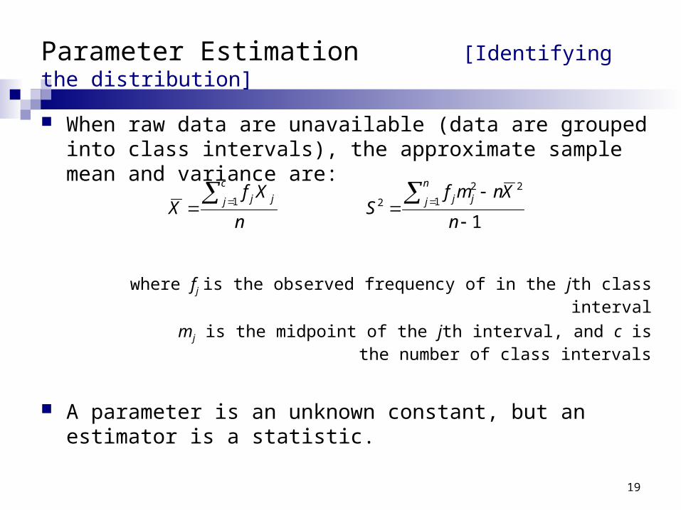
Parameter Estimation [Identifying the distribution]
When raw data are unavailable (data are grouped into class intervals), the approximate sample mean and variance are:
where fj is the observed frequency of in the jth class interval
mj is the midpoint of the jth interval, and c is the number of class intervals
A parameter is an unknown constant, but an estimator is a statistic.
1 1
22
21
n
XnmfS
n
XfX
n
j jj
c
j jj

9.3.2 on page 352
Numerical estimates of the distribution’s parameters are needed to reduce the family of distributions to a specific
distribution test the resulting hypothesis
Suggested estimators (Ch. 5) – see table 9.3
Examples 9.10 through 9.16 Parameter is an unknown constant, but Eestimator is a statistic (or random variable), because it
depends on the sample values
20

21
9.4 Goodness-of-Fit Tests [Identifying the distribution]
Conduct hypothesis testing on input data distribution using: Kolmogorov-Smirnov test Chi-square test
No single correct distribution in a real application exists. If very little data are available, it is unlikely to reject any candidate
distributions If a lot of data are available, it is likely to reject all candidate
distributions
22
Chi-Square test [Goodness-of-Fit Tests]
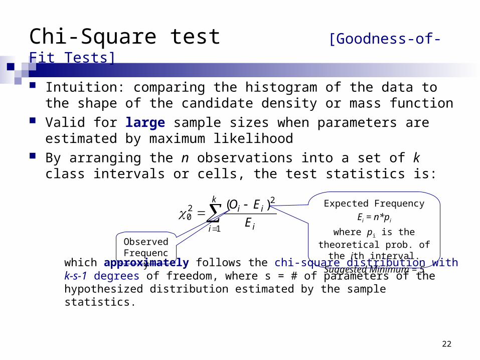
Intuition: comparing the histogram of the data to the shape of the candidate density or mass function
Valid for large sample sizes when parameters are estimated by maximum likelihood
By arranging the n observations into a set of k class intervals or cells, the test statistics is:
which approximately follows the chi-square distribution with k-s-1 degrees of freedom, where s = # of parameters of the hypothesized distribution estimated by the sample statistics.
k
i i
ii
E
EO
1
220
)(
Observed Frequency
Expected Frequency
Ei = n*pi
where pi is the theoretical prob. of the ith interval.
Suggested Minimum = 5
23
Chi-Square test [Goodness-of-Fit Tests]
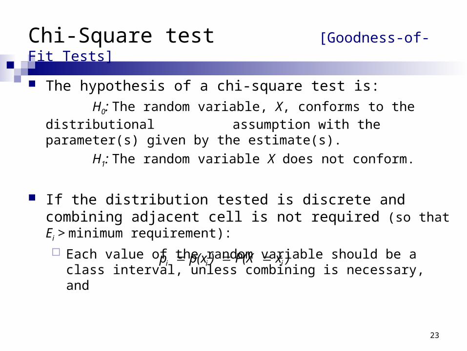
The hypothesis of a chi-square test is:
H0: The random variable, X, conforms to the distributional assumption with the parameter(s) given by the
estimate(s).
H1: The random variable X does not conform.
If the distribution tested is discrete and combining adjacent cell is not required (so that Ei > minimum requirement):
Each value of the random variable should be a class interval, unless combining is necessary, and ) x P(X ) p(x p iii
24
Chi-Square test [Goodness-of-Fit Tests]
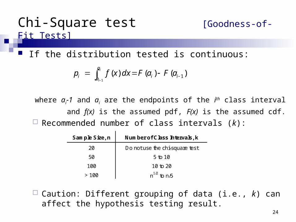
If the distribution tested is continuous:
where ai-1 and ai are the endpoints of the ith class interval
and f(x) is the assumed pdf, F(x) is the assumed cdf. Recommended number of class intervals (k):
Caution: Different grouping of data (i.e., k) can affect the hypothesis testing result.
)()( )( 11
ii
a
ai aFaFdxxf pi
i
Sample Size, n Number of Class Intervals, k
20 Do not use the chi-square test
50 5 to 10
100 10 to 20
> 100 n1/2 to n/5

25
Chi-Square test Ex 9.5,9.12.9.17
Vehicle Arrival : H0: the random variable is Poisson distributed.
H1: the random variable is not Poisson distributed.
Degree of freedom is k-s-1 = 7-1-1 = 5, hence, the hypothesis is rejected at the 0.05 level of significance.
!
)(
x
en
xnpEx
i
xi Observed Frequency, Oi Expected Frequency, Ei (Oi - Ei)2/Ei
0 12 2.61 10 9.62 19 17.4 0.153 17 21.1 0.84 19 19.2 4.415 6 14.0 2.576 7 8.5 0.267 5 4.48 5 2.09 3 0.810 3 0.3
> 11 1 0.1100 100.0 27.68
7.87
11.62 Combined because of min Ei
1.1168.27 25,05.0
20
26
Kolmogorov-Smirnov Test [Goodness-of-Fit Tests]
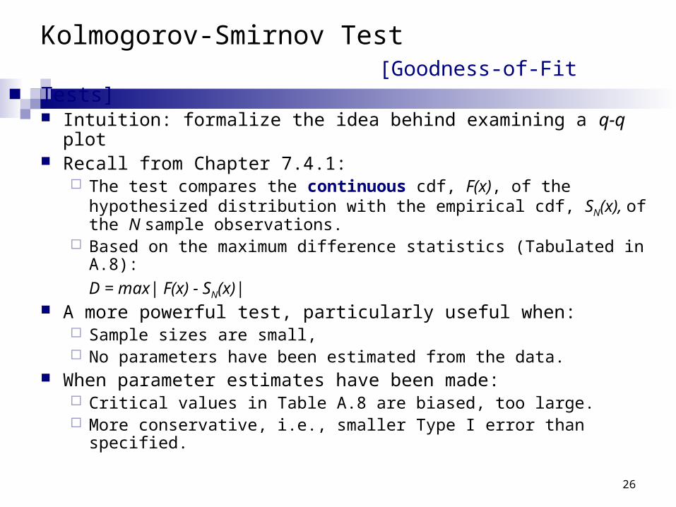
Intuition: formalize the idea behind examining a q-q plot Recall from Chapter 7.4.1:
The test compares the continuous cdf, F(x), of the hypothesized distribution with the empirical cdf, SN(x), of the N sample observations.
Based on the maximum difference statistics (Tabulated in A.8):
D = max| F(x) - SN(x)| A more powerful test, particularly useful when:
Sample sizes are small, No parameters have been estimated from the data.
When parameter estimates have been made: Critical values in Table A.8 are biased, too large. More conservative, i.e., smaller Type I error than specified.

27
p-Values and “Best Fits”[Goodness-of-Fit Tests]
p-value for the test statistics The significance level at which one would just reject H0 for the
given test statistic value. A measure of fit, the larger the better Large p-value: good fit Small p-value: poor fit
Vehicle Arrival Example (cont.): H0: data is Possion
Test statistics: , with 5 degrees of freedom p-value = 0.00004, meaning we would reject H0 with 0.00004
significance level, hence Poisson is a poor fit.
68.2720
28
p-Values and “Best Fits”[Goodness-of-Fit Tests]
Many software use p-value as the ranking measure to automatically determine the “best fit”. Things to be cautious about: Software may not know about the physical basis of the data,
distribution families it suggests may be inappropriate. Close conformance to the data does not always lead to the most
appropriate input model. p-value does not say much about where the lack of fit occurs
Recommended: always inspect the automatic selection using graphical methods.
29
9.5 Fitting a Non-stationary Poisson Process
Fitting a NSPP to arrival data is difficult, possible approaches: Fit a very flexible model with lots of parameters or Approximate constant arrival rate over some basic interval of time,
but vary it from time interval to time interval.
Suppose we need to model arrivals over time [0,T], our approach is the most appropriate when we can: Observe the time period repeatedly and Count arrivals / record arrival times.
Our focus
30
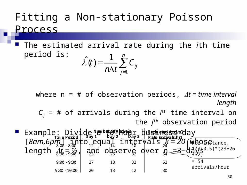
Fitting a Non-stationary Poisson Process
The estimated arrival rate during the ith time period is:
where n = # of observation periods, t = time interval length
Cij = # of arrivals during the ith time interval on the jth observation period
Example: Divide a 10-hour business day [8am,6pm] into equal intervals k = 20 whose length t = ½, and observe over n =3 days
n
jijC
tnt
1
1)(
Day 1 Day 2 Day 3
8:00 - 8:00 12 14 10 24
8:30 - 9:00 23 26 32 54
9:00 - 9:30 27 18 32 52
9:30 - 10:00 20 13 12 30
Number of Arrivals
Time PeriodEstimated Arrival Rate (arrivals/hr)
For instance, 1/3(0.5)*(23+26+32)
= 54 arrivals/hour
31
9.6 Selecting Model without Data
If data is not available, some possible sources to obtain information about the process are: Engineering data: often product or process has performance
ratings provided by the manufacturer or company rules specify time or production standards.
Expert option: people who are experienced with the process or similar processes, often, they can provide optimistic, pessimistic and most-likely times, and they may know the variability as well.
Physical or conventional limitations: physical limits on performance, limits or bounds that narrow the range of the input process.
The nature of the process. The uniform, triangular, and beta distributions are often used
as input models.
32
Selecting Model without Data
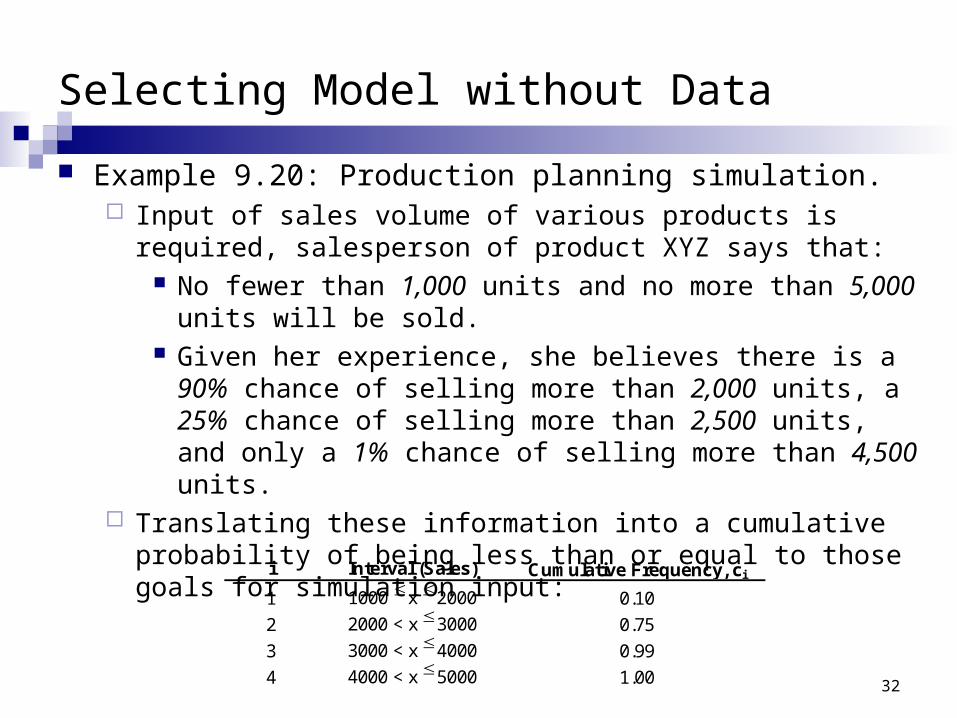
Example 9.20: Production planning simulation. Input of sales volume of various products is required, salesperson
of product XYZ says that: No fewer than 1,000 units and no more than 5,000 units will be
sold. Given her experience, she believes there is a 90% chance of
selling more than 2,000 units, a 25% chance of selling more than 2,500 units, and only a 1% chance of selling more than 4,500 units.
Translating these information into a cumulative probability of being less than or equal to those goals for simulation input:
i Interval (Sales) Cumulative Frequency, ci
1 1000 x 2000 0.10
2 2000 < x 3000 0.75
3 3000 < x 4000 0.99
4 4000 < x 5000 1.00

33
9.7 Multivariate and Time-Series Input Models
Multivariate: For example, lead time and annual demand for an inventory
model, increase in demand results in lead time increase, hence variables are dependent.
Time-series: For example, time between arrivals of orders to buy and sell
stocks, buy and sell orders tend to arrive in bursts, hence, times between arrivals are dependent.
34
Covariance and Correlation[Multivariate/Time Series]
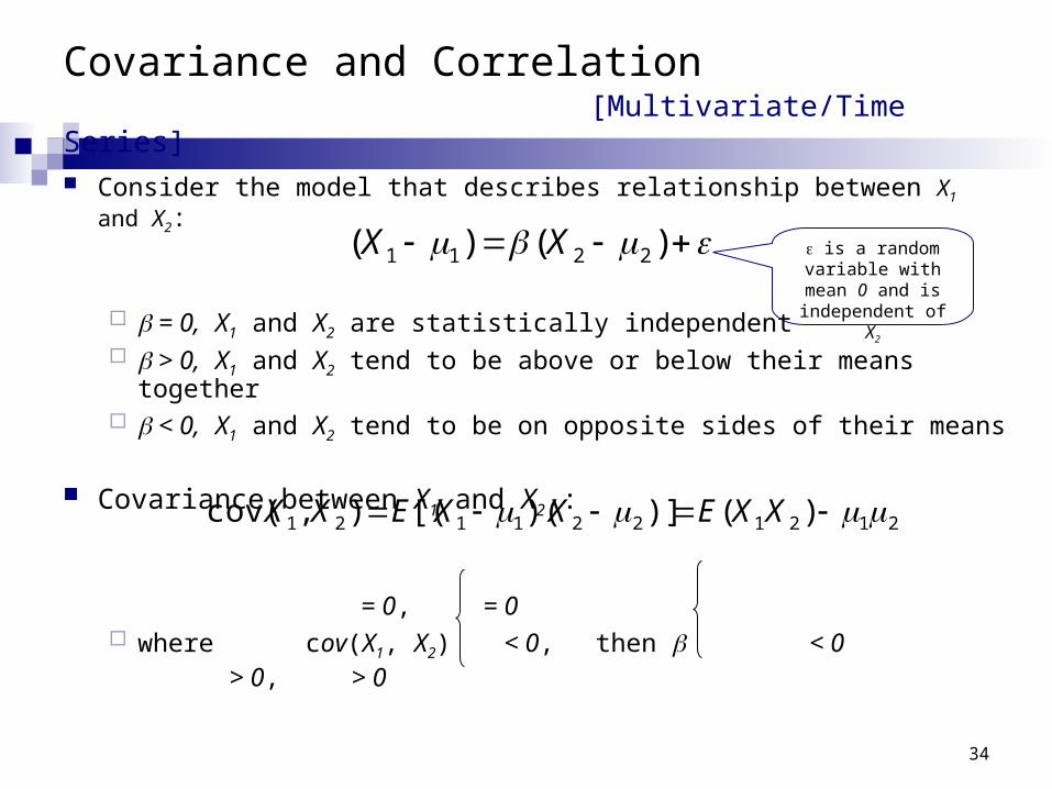
Consider the model that describes relationship between X1 and X2:
= 0, X1 and X2 are statistically independent > 0, X1 and X2 tend to be above or below their means together < 0, X1 and X2 tend to be on opposite sides of their means
Covariance between X1 and X2 :
= 0, = 0 where cov(X1, X2) < 0, then < 0
> 0, > 0
)()( 2211 XX
2121221121 )()])([(),cov( XXEXXEXX
is a random variable with mean 0 and is independent
of X2
35
Covariance and Correlation[Multivariate/Time Series]
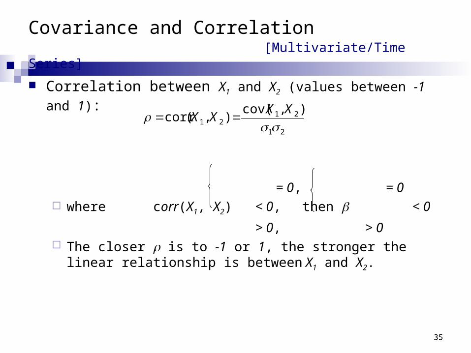
Correlation between X1 and X2 (values between -1 and 1):
= 0, = 0 where corr(X1, X2) < 0, then < 0
> 0, > 0 The closer is to -1 or 1, the stronger the linear relationship is
between X1 and X2.
21
2121
),cov(),(corr
XX
XX

36
Covariance and Correlation[Multivariate/Time Series]
A time series is a sequence of random variables X1, X2, X3, … , are identically distributed (same mean and variance) but dependent. cov(Xt, Xt+h) is the lag-h autocovariance
corr(Xt, Xt+h) is the lag-h autocorrelation
If the autocovariance value depends only on h and not on t, the time series is covariance stationary

37
Multivariate Input Models[Multivariate/Time Series]
If X1 and X2 are normally distributed, dependence between them can be modeled by the bivariate normal distribution with 1, 2, 1
2, 22 and correlation
To Estimate 1, 2, 12, 2
2, see “Parameter Estimation” (Section
9.3.2) To Estimate , suppose we have n independent and identically
distributed pairs (X11, X21), (X12, X22), … (X1n, X2n), then:
n
jjj
n
jjj
XXnXXn
XXXXn
XX
12121
1221121
ˆˆ1
1
)ˆ)(ˆ(1
1),v(oc
21
21
ˆˆ),v(oc
ˆ
XX
Sample deviation
38
Time-Series Input Models[Multivariate/Time Series]
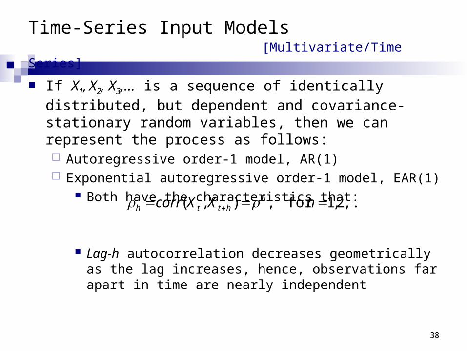
If X1, X2, X3,… is a sequence of identically distributed, but dependent and covariance-stationary random variables, then we can represent the process as follows: Autoregressive order-1 model, AR(1) Exponential autoregressive order-1 model, EAR(1)
Both have the characteristics that:
Lag-h autocorrelation decreases geometrically as the lag increases, hence, observations far apart in time are nearly independent
,...2,1for ,),( hXXcorr hhtth
39
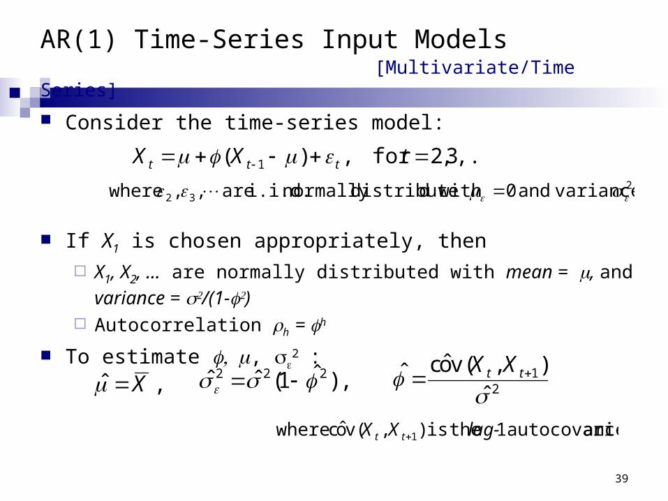
AR(1) Time-Series Input Models[Multivariate/Time Series]
Consider the time-series model:
If X1 is chosen appropriately, then
X1, X2, … are normally distributed with mean = , and variance =
/(1-) Autocorrelation h = h
To estimate , 2:
,...3,2for ,)( 1 tXX ttt 2
32 varianceand 0 with ddistributenormally i.i.d. are , , where
21
ˆ),v(ocˆ
tt XX
anceautocovari 1 theis ),v(oc where 1 lag-XX tt
, ˆ X , )ˆ1(ˆˆ 222
40
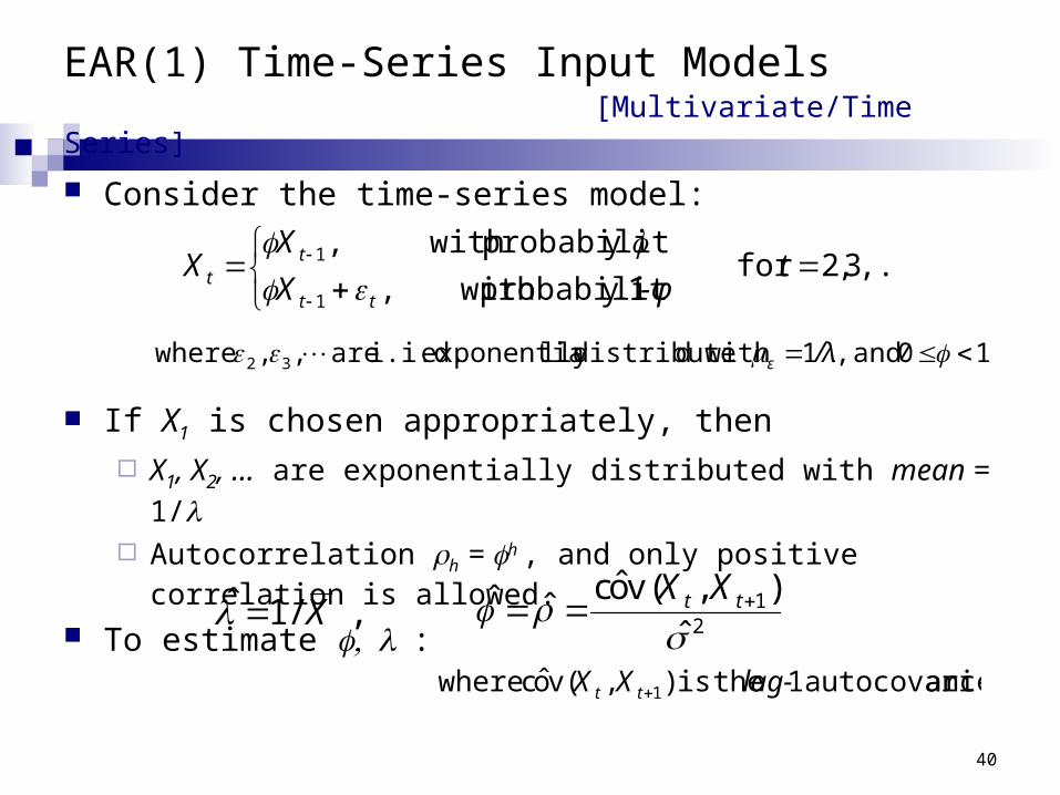
EAR(1) Time-Series Input Models[Multivariate/Time Series]
Consider the time-series model:
If X1 is chosen appropriately, then
X1, X2, … are exponentially distributed with mean = 1/ Autocorrelation h = h , and only positive correlation is allowed.
To estimate :
,...3,2for 1y probabilit with ,
y probabilit with ,
1
1
t-φX
XX
tt
tt
1 0 and ,1 with ddistributelly exponentia i.i.d. are , , where 32 /λε
21
ˆ),v(oc
ˆˆ
tt XX
anceautocovari 1 theis ),v(oc where 1 lag-XX tt
, /1ˆ X

Normal to Anything
The NORTA method on page 375
41
42
Summary
In this chapter, we described the 4 steps in developing input data models: Collecting the raw data Identifying the underlying statistical distribution Estimating the parameters Testing for goodness of fit