Chapter 8 Rootlocustechniques
47
Chapter 8: Root Locus Techniques
-
Upload
manjula-pandarikar -
Category
Documents
-
view
53 -
download
4
description
Control sytstem
Transcript of Chapter 8 Rootlocustechniques

Chapter 8: Root Locus Techniques

Muhamad Arfauz Bin A [email protected]
Robotic & Automation, FKP UTeM
2
Overview Introduction Defining the Root Locus Properties of the Root Locus Sketching the Root Locus Refining the Sketch An Example Transient Response Design via Gain Adjustment Generalized Root Locus Root Locus for Positive-Feedback Systems Pole Sensitivity

Muhamad Arfauz Bin A [email protected]
Robotic & Automation, FKP UTeM
3
Objectives Definition of a root locus How to sketch a root locus How to refine your sketch of a root locus How to use the root locus to find the poles of a
closed-loop system How to use the root locus to describe qualitatively the
changes in transient response and stability of a system as a system parameter is varied
How to use the root locus to design a parameter value to meet a transient response specification for systems of order 2 and higher

Muhamad Arfauz Bin A [email protected]
Robotic & Automation, FKP UTeM
4
Introduction What is root locus?
Root locus is a graphical representation of the closed-loop poles as a system parameter is varied
It can be used to describe qualitatively the performance of a system as various parameters are changed
It gives graphic representation of a system’s transient response and also stability
We can see the range of stability, instability, and the conditions that cause a system to break into oscillation

Muhamad Arfauz Bin A [email protected]
Robotic & Automation, FKP UTeM
5
The Control System Problem The poles of the open loop
transfer function are easily found by inspection and they do not change with changes in system gain. But the poles of the closed loop transfer function are more difficult to find and they change with changes in system gain
Consider the closed loop system in the next figurea) Closed loop systemb) Equivalent transfer function
Note: KG(s)H(s) = Open Loop Transfer Function, or loop gain

Muhamad Arfauz Bin A [email protected]
Robotic & Automation, FKP UTeM
6
If
G(s) = NG(s) / DG(s)
And
H(s) = NH(s) / DH(s)
Then
T(s) = KG(s) / 1 + K(s)H(s)
Therefore T(s) = KNG(s)DH(s) / DG(s)DH(s) + KNG(s)NH(s)
Observations: The zero of T(s) consist of the zeros of G(s) and The poles of H(s) The poles of T(s) are not immediately known without factoring the
denominator and they are a function of K Since the system’s performance depends on the knowledge of the
poles’ location, we will not be able to know the system performance readily
Root locus can be used to give us a picture of the poles of T(s) as the system gain, K, Varies

Muhamad Arfauz Bin A [email protected]
Robotic & Automation, FKP UTeM
7
Vector representation of complex number Vector has a magnitude
and a direction Complex number (σ +
jω) can be described in Cartesian coordinates or in polar form. It can also be represented by a vector
If a complex number is substituted into a complex function, F(s), another complex number will result
Muhamad Arfauz Bin A [email protected]
Robotic & Automation, FKP UTeM
8
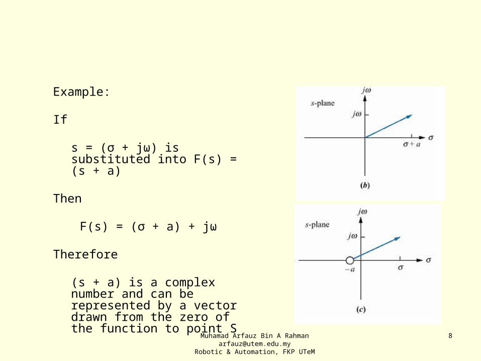
Example:
If
s = (σ + jω) is substituted into F(s) = (s + a)
Then
F(s) = (σ + a) + jω
Therefore
(s + a) is a complex number and can be represented by a vector drawn from the zero of the function to point S

Muhamad Arfauz Bin A [email protected]
Robotic & Automation, FKP UTeM
9
Draw the vector representation of (s + 7)|s5 + j2
Recall
F(s) =
Or
Where
∏ = Product
Or
F(s) = M∟θ (in polar form)
(s +z1)(s +z2)…(s + p1)(s + p2)…
F(s) = ∏ (s + zi) / ∏ (s + pj)m n
I =1 j =1

Muhamad Arfauz Bin A [email protected]
Robotic & Automation, FKP UTeM
10
Summary
M = ∏ zero lengths / ∏ pole lengths
Θ = Σ zero angles – Σ pole angles
n
jj
m
ii
ps
zsM
|)(|
|)(|
m
i
n
jji pszs )()(

Muhamad Arfauz Bin A [email protected]
Robotic & Automation, FKP UTeM
11
Given F(s) = , Find F(s) at the point s = -3 + j4Graphically:
For (s +1):(s + 1)|s-3 + j4
= (-3 + j4) + 1= -2 + j4= 4.47 ∟116.56o
Similarly:s|s-3 + j4 = 5 ∟126.9o
(s + 2)|s-3 + j4 = -1 + j4= 4.12 ∟
104.03o
ThereforeM∟θ = F(s)| s-3 + j4 = 4.47 / 5(4.12)
∟116.56o – 126.9o +104.03o
= 0.217 ∟ -114.3o
(s + 1)s(s + 2)

Muhamad Arfauz Bin A [email protected]
Robotic & Automation, FKP UTeM
12
Defining the Root LocusConsider the system
represented by block diagram next:
The C.L.T.F.
= K / s2 +10s + K
Where K = K1K2
If we plot the poles of the C.L.T.F. for value K = 0 50, we will obtain the following plots

Muhamad Arfauz Bin A [email protected]
Robotic & Automation, FKP UTeM
15
Observations: Root locus is the representation of the path of the closed loop poles as the gain is varied Root locus show the changes in the transient response as the gain K, variesFor 0 < K < 25
- poles are real and distinct (jω = 0)- Overdamped response
For K = 25- Poles are real and multiples- Critical response
For 25 < K < 50 (or K > 25)- Poles are complex conjugate- Underdamped response- Since Ts is inversely ∞ to the real part of the pole and the real part remains the same for K > 25- Therefore, the settling time, Ts, remains the same regardless of the value of gain (Note that Ts = 4 / σd)
For K > 25- as the gain increases, the damping ratio, ζ = cos θ decreases and thus the %OS decreases too- Note: %OS = e-[ζπ/√(1-ζ2)]*100- As the gain increases, the damped freq. of oscillation, ωd, which is the imaginary part of the complex pole also increase- Since peak time, Tp = π / ωd , thus an increase in ωd will result in an increase in Tp- Finally, since the root locus never crosses over into the RHP, the system is always stable, regardless of the value of gain
Muhamad Arfauz Bin A [email protected]
Robotic & Automation, FKP UTeM
16
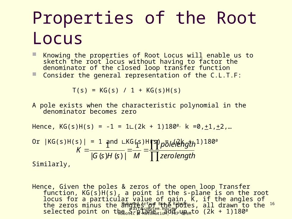
Properties of the Root Locus Knowing the properties of Root Locus will enable us to sketch the root locus
without having to factor the denominator of the closed loop transfer function Consider the general representation of the C.L.T.F:
T(s) = KG(s) / 1 + KG(s)H(s)
A pole exists when the characteristic polynomial in the denominator becomes zero
Hence, KG(s)H(s) = -1 = 1∟(2k + 1)1800, k =0,+1,+2,…
Or |KG(s)H(s)| = 1 and ∟KG(s)H(s) = (2k + 1)1800
Similarly,
Hence, Given the poles & zeros of the open loop Transfer function, KG(s)H(s), a point in the s-plane is on the root locus for a particular value of gain, K, if the angles of the zeros minus the angles of the poles, all drawn to the selected point on the S-plane, add up to (2k + 1)1800
lengthzerolengthpole
MsHsGK 1
|)()(|1

Muhamad Arfauz Bin A [email protected]
Robotic & Automation, FKP UTeM
17
Given a unity feedback system that has a the following forward transfer function:
a. Calculate the angle of G(s) at the point (-3 + j0) by finding the algebraic sum of angle of the vectors drawn from the zeros & poles of G(s) to the given point
b. Determine if the point specified in (a) is on the root locus
c. If the point is on the Root Locus, find the gain K using the lengths of the vectors
)134()2()( 2
sSsKsG

Muhamad Arfauz Bin A [email protected]
Robotic & Automation, FKP UTeM
18
)32)(32()2(
)134()2()( 2 jsjs
sKsS
sKsG
Σ angles = 1800 + θ1 + θ2 = 1800 -108.430 + 108.430 = 1800
Or
∟G(s)|s=-3j0= Σθzeros – Σθpoles
= 1800 – (-108.430 + 108.430) = 1800
Since the angle is 1800, the point is on Root Locus
101
)31)(31( 2222
ZerolengthPolelength
K
j3
-j3
-3 -2 -1
θ2
θ1
S-Plane
jω
σ

Muhamad Arfauz Bin A [email protected]
Robotic & Automation, FKP UTeM
19
Sketching the Root Locus Based on the properties of root locus, some rules are established to
enable us to sketch the Root Locus:

Muhamad Arfauz Bin A [email protected]
Robotic & Automation, FKP UTeM
20
No. of branches
The no. of branches of the R.L equals the number of closed-loop poles. (Since a branch is the path that one poles traverses.)
1st
2nd
Muhamad Arfauz Bin A [email protected]
Robotic & Automation, FKP UTeM
21
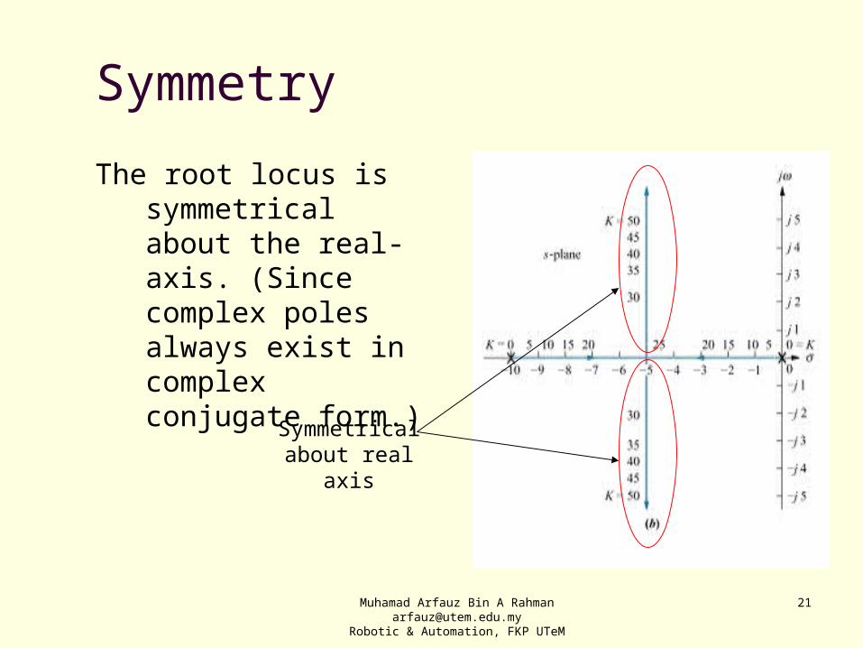
Symmetry
The root locus is symmetrical about the real-axis. (Since complex poles always exist in complex conjugate form.)
Symmetrical about real axis

Muhamad Arfauz Bin A [email protected]
Robotic & Automation, FKP UTeM
22
Real-axis segment
On the real-axis, for K>0, the root locus exists to the left of an odd number of real-axis, finite open-loop poles and/or finite open-loop zeros. (Due to the angle property of R-L.)
To the left of an odd number

Muhamad Arfauz Bin A [email protected]
Robotic & Automation, FKP UTeM
23
Starting & Ending Points
The root locus begins at the finite & infinite poles of G(s)H(s) & ends at the finite & infinite zeros of G(s)H(s).
Ending
Starting

Muhamad Arfauz Bin A [email protected]
Robotic & Automation, FKP UTeM
24
Concept of Infinite pole & zero Infinite pole: If the function approaches ∞ as s
approaches ∞, then the function has an infinite pole. Infinite zero: If the function approaches zero as s
approaches ∞, then, the function has an infinite zero Example: KG(s)H(s) = K / s(s + 1)(s + 2) This function has 3 finite poles at 0, -1, -2 & 3 infinite
zeros. Every function of s has an equal no. of poles & zeros
if we included the infinite poles & zeros as well as the finite poles & zeros.

Muhamad Arfauz Bin A [email protected]
Robotic & Automation, FKP UTeM
25
Behavior at infinity The root locus approaches straight lines as
asymptotes as the locus approaches infinity. The equation of the asymptotes is given by the real-
axis intercept, σa & angle θa :
Where k = 0, +1, +2, + 3, and the angle is given in radians w.r.t. the positive extension of the real-axis.
zerosfinitepolesfinitek
zerosfinitepolesfinitezerosfinitepolesfinite
a
a
##)12(##

Muhamad Arfauz Bin A [email protected]
Robotic & Automation, FKP UTeM
26
Example: Sketch the root locus for the system shown
Notice that there are 4 finite poles & 1 finite zero.
Thus there will be 3 infinite zeros.
Calculate the asymptotes of the infinite zeros:
Intercept on real-axis.2
35
1
03
##)12(
34
14)3()421(##
kfor
kfor
kfor
zerosfinitepolesfinitek
zerosfinitepolesfinitezerosfinitepolesfinite
a
a
a

Muhamad Arfauz Bin A [email protected]
Robotic & Automation, FKP UTeM
27
Root locus and asymptotes for the system of previous example
Real axis intercept
Π /3
5Π /3

Muhamad Arfauz Bin A [email protected]
Robotic & Automation, FKP UTeM
29
Real-Axis Breakaway & Break-in Points
Breakaway point is the point where the locus leaves the real-axis. (-σ1 in the figure)
Break-in point is the point where the locus returns to the real-axis.(σ2 in the figure)
Muhamad Arfauz Bin A [email protected]
Robotic & Automation, FKP UTeM
30
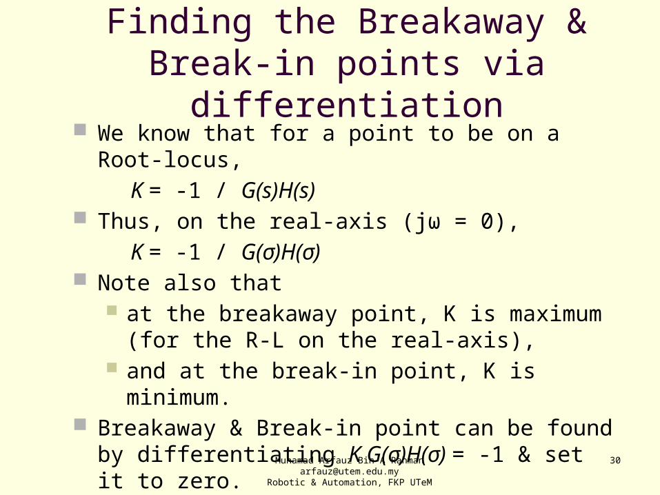
Finding the Breakaway & Break-in points via differentiation
We know that for a point to be on a Root-locus, K = -1 / G(s)H(s)
Thus, on the real-axis (jω = 0), K = -1 / G(σ)H(σ)
Note also that at the breakaway point, K is maximum (for the R-L
on the real-axis), and at the break-in point, K is minimum.
Breakaway & Break-in point can be found by differentiating K G(σ)H(σ) = -1 & set it to zero.

Muhamad Arfauz Bin A [email protected]
Robotic & Automation, FKP UTeM
31
Find the breakaway & break-in points for the root locus shown
82.3,45.1
0)158(
)612611(
1)23(
)158(
)()(1)()(,&
)23()158(
)2)(1()5)(3()()(
22
2
2
2
2
2
dk
K
HKGsHsKGaxisrealtheonlocusroottheOn
ssssK
ssssKsHsKG
LocusRoottheFrom
0)(:
dGtakeweifresultsamethegetwillWeNote

Muhamad Arfauz Bin A [email protected]
Robotic & Automation, FKP UTeM
32
Finding Breakaway & Break-in Points by transition method
This method eliminates the step of differentiation.
Derivation in Appendix J.2. on CD-Rom.
This method states that: Breakaway & break-in
points satisfy the following relationship:
Where Zi & Pi are the negative of the zero & pole values, respectively, of G(s)H(s).
n
i
m
i pz 11
11
82.3,45.10612611
21
11
51
31
)2)(1()5)(3()()(
Re
2
ssssKsHsKG
methodthiswithexamplepreviousthepeat

Muhamad Arfauz Bin A [email protected]
Robotic & Automation, FKP UTeM
33
Finding the jω axis crossings Jω axis crossing is a point on the R-L that separates the stable
operation of the system from the unstable operation. The value of ω at the axis crossing yields the frequency of oscillation. The gain at the jω axis crossing yields the max. positive gain for
system stability.
Jω-axis crossing can be found by using Routh-Hurwitz criterion as follows:
Forcing a row of zeros in the Routh Table will yield the gain. Going back one row to the even polynomial equation & solving for the
roots yields the frequency at the imaginary axis crossing.
(Recall that a row of zeros in the Routh Table indicates the existence of poles on the jω axis.)

Muhamad Arfauz Bin A [email protected]
Robotic & Automation, FKP UTeM
34
For the system shown, find the frequency & gain, K, for which the root locus crosses the imaginary axis. For what range of K is the system stable?
KsKssssKsT
where
sHsHsG
sGsTofFTLC
3)8(147)3()(
1)(,)()(1
)()(...
234

Muhamad Arfauz Bin A [email protected]
Robotic & Automation, FKP UTeM
35
Construction of Routh table

Muhamad Arfauz Bin A [email protected]
Robotic & Automation, FKP UTeM
36
Continuation of Previous Problem Solving
For +ve K, only s1 row can be all zeros.
Let -K2 -65K+720 / 90-K = 0 to find value of K on jω-axis.-K2 -65K+720 = 0K = 9.65
To find the frequency on the jω axis crossing, form the even polynomial by using the s2 row & with K= 9.65,
(90 -K)s2 + 21K = 080.35s2 + 202.7 = 0s2 = -202.7 / 80.35s = +j1.59
The root-locus crosses the jω axis at + j1.59 at a gain of 9.65
The system is stable for 0 < K < 9.65

Muhamad Arfauz Bin A [email protected]
Robotic & Automation, FKP UTeM
37
Angle of departure & arrival from complex poles & zeros
Recall that a condition for a point on the s-plane to be on the root locus is that the angles of the zeros minus the angles of the poles, all drawn to the selected point on the s-plane, add up to (2k + 1) 180°.
Example∟KG(s)H (s) = (2k + 1 ) 180°
Consider the next Figure:

Muhamad Arfauz Bin A [email protected]
Robotic & Automation, FKP UTeM
38
Angle of departure & arrival Assume ε is a point on the root
locus close to a complex pole.
Sum of all angles drawn from all other poles & zeros to the pole that is near to ε is:
-θ1, + θ2 + θ3 – θ4 – θ5 + θ6 =(2k+I)180°
The angle of departure is:
θ1 = θ2 + θ3 – θ4 – θ5,+ θ6 - (2k+1)180°
Similarly, for complex zero:
-θ1 + θ2 + θ3 – θ4 – θ5 + θ6 = (2k+I)180°
The angle of arrival is:
θ2 = θ1 - θ3 + θ4 + θ5,- θ6 + (2k+1)180°

Muhamad Arfauz Bin A [email protected]
Robotic & Automation, FKP UTeM
39
Example:Given the unity feedback system, find the angle of departure from the complex poles & sketch the root locus
)11)(11)(3()2()()(
1)(,)22)(3(
)2()()( 2
jsjsssKsHsKG
where
sHsSs
sKsHsKG
Root locus for the systemshowing angle of departure

Muhamad Arfauz Bin A [email protected]
Robotic & Automation, FKP UTeM
40
Continuation of Previous Problem Solving
)(4.108
4.1086.251
1805.264590
18021tan
11tan90
)0(180180)12(
0
00
00001
01101
004321
axisrealtheaboutsymmetryispolecomplextheofdepartureofangleThe
kk
Muhamad Arfauz Bin A [email protected]
Robotic & Automation, FKP UTeM
41
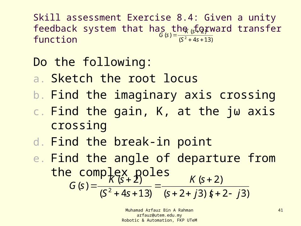
Skill assessment Exercise 8.4: Given a unity feedback system that has the forward transfer function
Do the following:a. Sketch the root locusb. Find the imaginary axis crossingc. Find the gain, K, at the jω axis crossingd. Find the break-in pointe. Find the angle of departure from the
complex poles
)134()2()( 2
sSsKsG
)32)(32()2(
)134()2()( 2 jsjs
sKsS
sKsG

Muhamad Arfauz Bin A [email protected]
Robotic & Automation, FKP UTeM
42
An Example Sketching the root locus & Finding the critical points
Find the exact point and gain where the locus crosses the 0.45 damping ratio line
Find the exact point and gain where the locus crosses the jw-axis
Find the breakaway point on the real axis Find the range K within which the system is stable

Muhamad Arfauz Bin A [email protected]
Robotic & Automation, FKP UTeM
43
Transient Response Design via Gain Adjustment Use Second order approximation which satisfy the following conditions:
Higher order poles are much farther into the left half of the s-plane than the dominant second order pair of poles. The response that results from a higher order pole does not appreciably change the transient response expected from the dominant second order poles
Closed loop zeros near the closed loop second order pole pair are nearly cancelled by the close proximity of higher order closed loop poles
Closed loop zeros not cancelled by the close proximity of higher order closed loop poles are far removed from the closed loop second order pole pair

Muhamad Arfauz Bin A [email protected]
Robotic & Automation, FKP UTeM
44
Please Read!!!
Generalized Root Locus Root Locus for Positive-Feedback Systems

Muhamad Arfauz Bin A [email protected]
Robotic & Automation, FKP UTeM
45
Pole Sensitivity Since Root Locus is a plot of the Closed Loop Poles
as a system parameter is varied any change in the parameter will change the system performance too!
Root Locus exhibits nonlinear relationship between gain and pole Along some sections of the RL – very small changes in
gain yield very large changes in pole location and hence performance High Sensitivity to changes in gain
Along other sections of the RL – very large changes in gain yield very small changes in pole location Low Sensitivity to changes in gain
Preferences Low Sensitivity to changes in gain

Muhamad Arfauz Bin A [email protected]
Robotic & Automation, FKP UTeM
46
Applying Definition of sensitivity root sensitivity is the ratio of the fractional change in a closed loop pole to the fractional change in a system parameter (e.g. gain)
Using Equation in Ch. 7, sensitivity of a closed loop pole, s, to gain, K:
S is the current pole location K is the current gain
Converting the partials to finite increments, the actual change in the closed loop pole can be approximate as:
Δs is the change in pole location ΔK/K is the fractional Change in gain K
Ks
sKS Ks
:
KKSsS Ks
)( :

Muhamad Arfauz Bin A [email protected]
Robotic & Automation, FKP UTeM
47
Example: Root Sensitivity of a closed loop system to gain variations Find the root sensitivity of the system in Figure 8.4 at
s = -9.47 and -5+j5. also calculate the change in the pole location for a 10% change in K
System C.E. found from closed loop transfer function denominator is s2 +10s + K = 0
ateDifferenti