CHAPTER 8 REVIEW: BINOMIAL AND GEOMETRIC DISTRIBUTIONS

Kristy Fan and Karey Duane

Overview

You should be able to:

Identify a random variable as a binomial or geometric

Use the formula to determine binomial or geometric probabilities

Calculate cumulative distribution functions for binomial random variables and geometric random variables and construct cumulative distribution tables and histograms

Calculate means, expected values, and standard deviations of binomial and geometric variables

Use Normal approximation to the binomial distribution to compute probabilities

Binomial vs. Geometric Variables

Counts the number of successes X in a given number of trials n

Counts the number of trials X needed to get the first success

Binomial Geometric

Both are discrete random variables.

Binomial Setting

Each observation falls into one of two categories: success or failure

Observations are all independent: knowing the result of one observation tells you nothing about the others

Probability of success (p) is the same for each observation

Fixed number (n) of observations

Variables and Parameters

X= binomial random variable that is the number of successes

Probability distribution of X is a binomial distribution

Parameters:

n= number of observations

p= probability of success of any one observation

0<X<n, whole numbers only

Sampling Distribution

choose an SRS of size n from the population with proportion p of successes

when population is at least 10 times larger than the sample (N>10n), X number of successes in sample has approximate binomial distribution with parameters n and p

X = B(n,p)

Binomial Coefficient

Number of ways of arranging k successes among n observations

Note: not n divided by k, but n choose k

nkknk

n

k

n0,

)!(!

!

Combination Shortcuts

Binomial Probability

P(X=k)

Binomial coefficient X probability of any arrangement of k success

X=# of successes

n=# of observations

p= probability of success each time

k= a value of x

)1()( ppknk

k

nkXP

pdf vs. cdf

Probability distribution function (pdf)

assigns a probability to each value of X

Cumulative distribution function (cdf)

calculates the sum of the probabilities for 0,1,2…. up to the value of X, including the value of X

calculates the probability of obtaining at most X successes in n trials

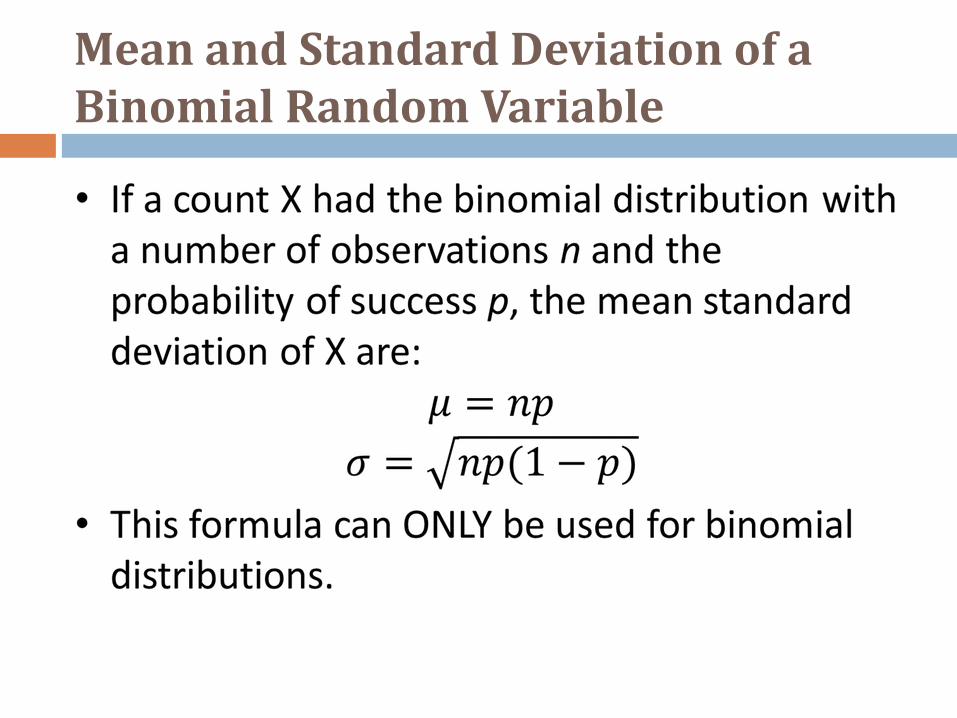
Mean and Standard Deviation of a Binomial Random Variable

Normal Approximations for Binomial Distributions

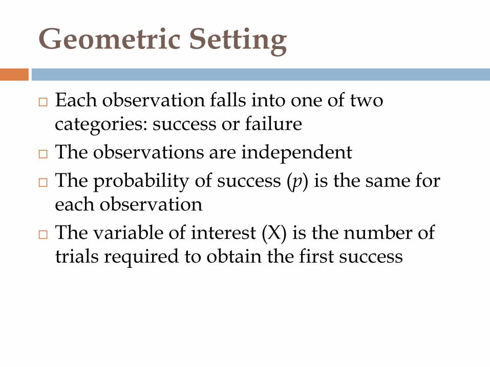
Geometric Setting

Each observation falls into one of two categories: success or failure

The observations are independent

The probability of success (p) is the same for each observation

The variable of interest (X) is the number of trials required to obtain the first success

Rule for Calculating Geometric Probabilities

Mean and Standard Deviation of a Geometric Random Variable

Calculator Keystrokes

To… Do This…

Calculate binomial probability of X 2nd→vars→A: binompdf(

P(X=k)=binompdf(n,p,X)

Calculate binomial probability up to or

equal to X

2nd→vars→A: binomcdf(

P(X=k)=binomcdf(n,p,X)

Simulate many trials in a binomial setting Math→PRB→7: randBin(

randBin(1,p,n)

1=success; 0=failure

Count the number of successes in n trials Simulate many trials

STO→L1: sum (L1)

Execute Math→PRB→3: nCr

n nCr k

Calculate geometric probability 2nd→VARS→E:geometpdf(

geometpdf(p of failing, n)

k

n