Chapter 8

Interference

Version 0408.2.K.pdf, 22 November 2004. [Changes since 0408.1.k: minor typos corrected]Please send comments, suggestions, and errata via email to kip@tapir.caltech.edu and tordb@caltech.edu, or on paper to Kip Thorne, 130-33 Caltech, Pasadena CA 91125

8.1 Overview

In the last chapter, we considered superpositions of waves that pass through a (typicallylarge) aperture. The foundation for our analysis was an expression for the field at a chosenpoint P as a sum of contributions from all points on a closed surface surrounding P. The spa-tially varying field pattern resulting from this superposition of many different contributionswas called diffraction.

In this chapter, we continue our discussion of the effects of superposition, but for themore special case where only two or at most several discrete beams are being superposed.For this special case one uses the term interference rather than diffraction. Interferenceis important in a wide variety of practical instruments designed to measure or utilize thespatial and temporal structures of electromagnetic radiation. However interference is not justof practical importance. Attempting to understand it forces us to devise ways of describingthe radiation field that are independent of the field’s origin and independent of the meansby which it is probed; and such descriptions lead us naturally to the concept of coherence(Sec. 8.2).

The light from a distant, monochromatic point source is effectively a plane wave; we callit “perfectly coherent” radiation. In fact, there are two different types of coherence present:lateral or spatial coherence (coherence in the angular structure of the radiation field), andtemporal or longitudinal coherence (coherence in the field’s temporal structure, which clearlymust imply something also about its frequency structure). We see in Sec. 8.2 that for bothtypes of coherence there is a measurable quantity, called the degree of coherence, that isthe Fourier transform of either the angular intensity distribution or the spectrum of theradiation.

Interspersed with our development of the theory of coherence are applications to thestellar interferometer by which Michelson measured the diameters of Jupiter’s moons andseveral bright stars using spatial coherence (Sec. 8.2.5), and a Michelson interferometer

1

2

a

a

F

Fmax

Fmin

Fmax

+ Fmin

arg ( )

(c)(b)(a)

Fmax

Fmin=

θ

θ

θ

−

F

θ

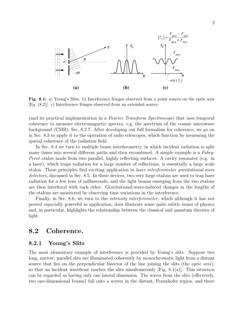
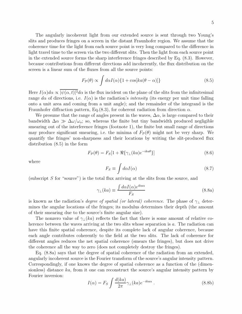
Fig. 8.1: a) Young’s Slits. b) Interference fringes observed from a point source on the optic axis[Eq. (8.2)]. c) Interference fringes observed from an extended source.

(and its practical implementation in a Fourier Transform Spectroscope) that uses temporalcoherence to measure electromagnetic spectra, e.g. the spectrum of the cosmic microwavebackground (CMB); Sec. 8.2.7. After developing our full formalism for coherence, we go onin Sec. 8.3 to apply it to the operation of radio telescopes, which function by measuring thespatial coherence of the radiation field.

In Sec. 8.4 we turn to multiple beam interferometry, in which incident radiation is splitmany times into several different paths and then recombined. A simple example is a Fabry-Perot etalon made from two parallel, highly reflecting surfaces. A cavity resonator (e.g. ina laser), which traps radiation for a large number of reflections, is essentially a large scaleetalon. These principles find exciting application in laser interferometer gravitational-wavedetectors, discussed in Sec. 8.5. In these devices, two very large etalons are used to trap laserradiation for a few tens of milliseconds, and the light beams emerging from the two etalonsare then interfered with each other. Gravitational-wave-induced changes in the lengths ofthe etalons are monitored by observing time variations in the interference.

Finally, in Sec. 8.6, we turn to the intensity interferometer, which although it has notproved especially powerful in application, does illustrate some quite subtle issues of physicsand, in particular, highlights the relationship between the classical and quantum theories oflight.

8.2 Coherence.

8.2.1 Young’s Slits

The most elementary example of interference is provided by Young’s slits. Suppose twolong, narrow, parallel slits are illuminated coherently by monochromatic light from a distantsource that lies on the perpendicular bisector of the line joining the slits (the optic axis),so that an incident wavefront reaches the slits simultaneously [Fig. 8.1(a)]. This situationcan be regarded as having only one lateral dimension. The waves from the slits (effectively,two one-dimensional beams) fall onto a screen in the distant, Fraunhofer region, and there

3

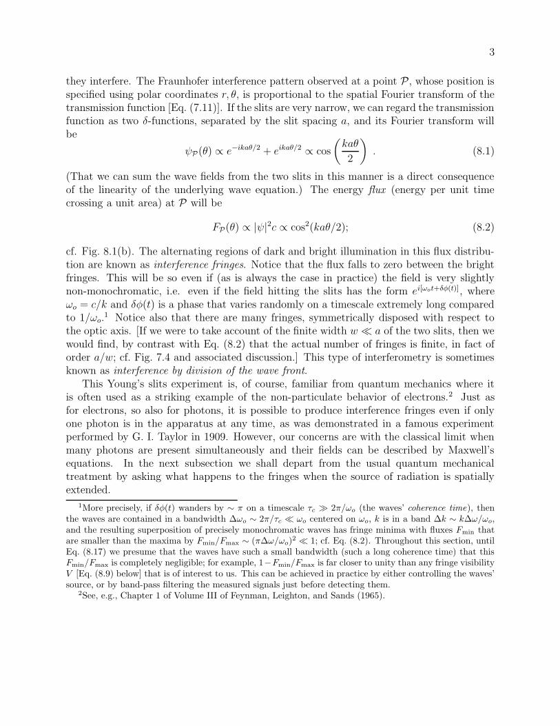
they interfere. The Fraunhofer interference pattern observed at a point P, whose position isspecified using polar coordinates r, θ, is proportional to the spatial Fourier transform of thetransmission function [Eq. (7.11)]. If the slits are very narrow, we can regard the transmissionfunction as two δ-functions, separated by the slit spacing a, and its Fourier transform willbe

ψP(θ) ∝ e−ikaθ/2 + eikaθ/2 ∝ cos

(

kaθ

2

)

. (8.1)

(That we can sum the wave fields from the two slits in this manner is a direct consequenceof the linearity of the underlying wave equation.) The energy flux (energy per unit timecrossing a unit area) at P will be

FP(θ) ∝ |ψ|2c ∝ cos2(kaθ/2); (8.2)

cf. Fig. 8.1(b). The alternating regions of dark and bright illumination in this flux distribu-tion are known as interference fringes. Notice that the flux falls to zero between the brightfringes. This will be so even if (as is always the case in practice) the field is very slightlynon-monochromatic, i.e. even if the field hitting the slits has the form ei[ωot+δφ(t)], whereωo = c/k and δφ(t) is a phase that varies randomly on a timescale extremely long comparedto 1/ωo.

1 Notice also that there are many fringes, symmetrically disposed with respect tothe optic axis. [If we were to take account of the finite width w a of the two slits, then wewould find, by contrast with Eq. (8.2) that the actual number of fringes is finite, in fact oforder a/w; cf. Fig. 7.4 and associated discussion.] This type of interferometry is sometimesknown as interference by division of the wave front.

This Young’s slits experiment is, of course, familiar from quantum mechanics where itis often used as a striking example of the non-particulate behavior of electrons.2 Just asfor electrons, so also for photons, it is possible to produce interference fringes even if onlyone photon is in the apparatus at any time, as was demonstrated in a famous experimentperformed by G. I. Taylor in 1909. However, our concerns are with the classical limit whenmany photons are present simultaneously and their fields can be described by Maxwell’sequations. In the next subsection we shall depart from the usual quantum mechanicaltreatment by asking what happens to the fringes when the source of radiation is spatiallyextended.

1More precisely, if δφ(t) wanders by ∼ π on a timescale τc 2π/ωo (the waves’ coherence time), thenthe waves are contained in a bandwidth ∆ωo ∼ 2π/τc ωo centered on ωo, k is in a band ∆k ∼ k∆ω/ωo,and the resulting superposition of precisely monochromatic waves has fringe minima with fluxes Fmin thatare smaller than the maxima by Fmin/Fmax ∼ (π∆ω/ωo)

2 1; cf. Eq. (8.2). Throughout this section, untilEq. (8.17) we presume that the waves have such a small bandwidth (such a long coherence time) that thisFmin/Fmax is completely negligible; for example, 1−Fmin/Fmax is far closer to unity than any fringe visibilityV [Eq. (8.9) below] that is of interest to us. This can be achieved in practice by either controlling the waves’source, or by band-pass filtering the measured signals just before detecting them.

2See, e.g., Chapter 1 of Volume III of Feynman, Leighton, and Sands (1965).

4

8.2.2 Interference with an Extended Source: Van Cittert-Zernike

Theorem.

We shall approach the topic of extended sources in steps. Our first step was taken in the lastsubsection, where we dealt with an idealized, single, incident plane wave, such as might beproduced by an ideal, distant laser. We have called this type of radiation perfectly coherent,which we have implicitly taken to mean that the field oscillates with a fixed frequency ωo anda randomly but very slowly varying phase δφ(t) (see footnote 1), and thus, for all practicalpurposes, there is a time-independent phase difference between any two points within theregion under consideration.

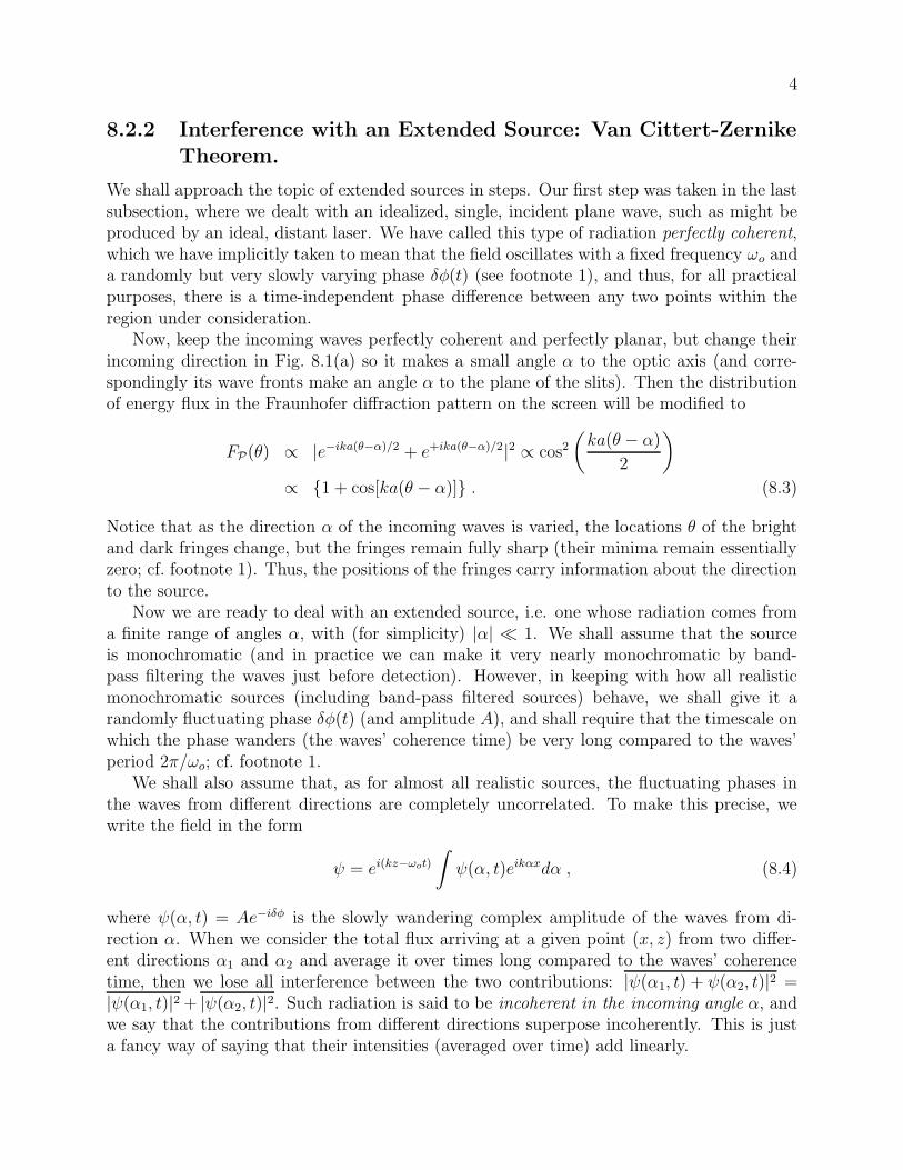
Now, keep the incoming waves perfectly coherent and perfectly planar, but change theirincoming direction in Fig. 8.1(a) so it makes a small angle α to the optic axis (and corre-spondingly its wave fronts make an angle α to the plane of the slits). Then the distributionof energy flux in the Fraunhofer diffraction pattern on the screen will be modified to

FP(θ) ∝ |e−ika(θ−α)/2 + e+ika(θ−α)/2|2 ∝ cos2

(

ka(θ − α)

2

)

∝ 1 + cos[ka(θ − α)] . (8.3)

Notice that as the direction α of the incoming waves is varied, the locations θ of the brightand dark fringes change, but the fringes remain fully sharp (their minima remain essentiallyzero; cf. footnote 1). Thus, the positions of the fringes carry information about the directionto the source.

Now we are ready to deal with an extended source, i.e. one whose radiation comes froma finite range of angles α, with (for simplicity) |α| 1. We shall assume that the sourceis monochromatic (and in practice we can make it very nearly monochromatic by band-pass filtering the waves just before detection). However, in keeping with how all realisticmonochromatic sources (including band-pass filtered sources) behave, we shall give it arandomly fluctuating phase δφ(t) (and amplitude A), and shall require that the timescale onwhich the phase wanders (the waves’ coherence time) be very long compared to the waves’period 2π/ωo; cf. footnote 1.

We shall also assume that, as for almost all realistic sources, the fluctuating phases inthe waves from different directions are completely uncorrelated. To make this precise, wewrite the field in the form

ψ = ei(kz−ωot)

∫

ψ(α, t)eikαxdα , (8.4)

where ψ(α, t) = Ae−iδφ is the slowly wandering complex amplitude of the waves from di-rection α. When we consider the total flux arriving at a given point (x, z) from two differ-ent directions α1 and α2 and average it over times long compared to the waves’ coherencetime, then we lose all interference between the two contributions: |ψ(α1, t) + ψ(α2, t)|2 =|ψ(α1, t)|2 + |ψ(α2, t)|2. Such radiation is said to be incoherent in the incoming angle α, andwe say that the contributions from different directions superpose incoherently. This is justa fancy way of saying that their intensities (averaged over time) add linearly.

5

The angularly incoherent light from our extended source is sent through two Young’sslits and produces fringes on a screen in the distant Fraunhofer region. We assume that thecoherence time for the light from each source point is very long compared to the difference inlight travel time to the screen via the two different slits. Then the light from each source pointin the extended source forms the sharp interference fringes described by Eq. (8.3). However,because contributions from different directions add incoherently, the flux distribution on thescreen is a linear sum of the fluxes from all the source points:

FP(θ) ∝∫

dαI(α)1 + cos[ka(θ − α)] (8.5)

Here I(α)dα ∝ |ψ(α, t)|2dα is the flux incident on the plane of the slits from the infinitesimalrange dα of directions, i.e. I(α) is the radiation’s intensity (its energy per unit time fallingonto a unit area and coming from a unit angle); and the remainder of the integrand is theFraunhofer diffraction pattern, Eq.(8.3), for coherent radiation from direction α.

We presume that the range of angles present in the waves, ∆α, is large compared to theirbandwidth ∆α ∆ω/ωo; so, whereas the finite but tiny bandwidth produced negligiblesmearing out of the interference fringes (footnote 1), the finite but small range of directionsmay produce significant smearing, i.e. the minima of FP(θ) might not be very sharp. Wequantify the fringes’ non-sharpness and their locations by writing the slit-produced fluxdistribution (8.5) in the form

FP(θ) = FS[1 + <γ⊥(ka)e−ikaθ] (8.6)

where

FS ≡∫

dαI(α) (8.7)

(subscript S for “source”) is the total flux arriving at the slits from the source, and

γ⊥(ka) ≡∫

dαI(α)eikaα

FS

(8.8a)

is known as the radiation’s degree of spatial (or lateral) coherence. The phase of γ⊥ deter-mines the angular locations of the fringes; its modulus determines their depth (the amountof their smearing due to the source’s finite angular size).

The nonzero value of γ⊥(ka) reflects the fact that there is some amount of relative co-herence between the waves arriving at the two slits whose separation is a. The radiation canhave this finite spatial coherence, despite its complete lack of angular coherence, becauseeach angle contributes coherently to the field at the two slits. The lack of coherence fordifferent angles reduces the net spatial coherence (smears the fringes), but does not drivethe coherence all the way to zero (does not completely destroy the fringes).

Eq. (8.8a) says that the degree of spatial coherence of the radiation from an extended,angularly incoherent source is the Fourier transform of the source’s angular intensity pattern.Correspondingly, if one knows the degree of spatial coherence as a function of the (dimen-sionless) distance ka, from it one can reconstruct the source’s angular intensity pattern byFourier inversion:

I(α) = FS

∫

d(ka)

2πγ⊥(ka)e−ikaα . (8.8b)

6

The two Fourier relations (8.8a), (8.8b) are called the van Cittert-Zernike Theorem. InEx. 8.7, we shall see that this theorem is a complex-variable version of Chap. 5’s Wiener-Khintchine Theorem for random processes.

Because of its relationship to the source’s angular intensity pattern, the degree of spatialcoherence is of great practical importance. For a given choice of ka (a given distance betweenthe slits), γ⊥ is a complex number that one can read off the interference fringes of Eq. (8.6)and Fig. 8.1(c) as follows: Its modulus is

|γ⊥| ≡ V =Fmax − Fmin

Fmax + Fmin(8.9)

where Fmax and Fmin are the maximum and minimum values of the flux FP on the screen;and its phase arg(γ⊥) is ka times the displacement ∆θ of the centers of the bright fringesfrom the optic axis. The modulus is called the fringe visibility because of its measuringthe fractional contrast in the fringes [Eq. (8.9)], and this name is the reason for the symbolV . Analogously, the complex quantity γ⊥ (or a close relative) is sometimes known as thecomplex fringe visibility. Notice that V can lie anywhere in the range from zero (no contrast;fringes completely undetectable) to unity (monochromatic plane wave; contrast as large aspossible). When the phase arg(γ⊥) of the complex visibility (degree of coherence) is zero,there is a bright fringe precisely on the optic axis. This will be the case, e.g., for a sourcethat is symmetric about the optic axis. If the symmetry point of such a source is graduallymoved off the optic axis by an angle δα, the fringe pattern will shift correspondingly byδα = δθ, and this will show up as a corresponding shift in the argument of the fringevisibility, arg(γ⊥) = kaδα.

The above analysis shows that Young’s slits are nicely suited to measuring both themodulus and the phase of the complex fringe visibility (the degree of spatial coherence) ofthe radiation from an extended source.

8.2.3 More General Formulation of Spatial Coherence; Lateral

Coherence Length

It is not necessary to project the light onto a screen to determine the contrast and angularpositions of the fringes. For example, if we had measured the field at the locations of the twoslits, we could have combined the signals electronically and cross correlated them numericallyto determine what the fringe pattern would be with slits. All we are doing with the Young’sslits is sampling the wave field at two different points, which we now shall label 1 and 2.Observing the fringes corresponds to adding a phase φ (= kaθ) to the field at one of thepoints and then adding the fields and measuring the flux ∝ |ψ1 +ψ2e

iφ|2 averaged over manyperiods. Now, since the source is far away, the rms value of the wave field will be the sameat the two slits, |ψ1|2 = |ψ2|2 ≡ |ψ|2. We can therefore express this time averaged flux in thesymmetric-looking form

FP(φ) ∝ (ψ1 + ψ2eiφ)(ψ∗1 + ψ∗

2e−iφ)

∝ 1 + <(

ψ1ψ∗2

|ψ|2e−iφ

)

. (8.10)

7

Here a bar denotes an average over times long compared to the coherence times for ψ1 andψ2. Comparing with Eq. (8.6) and using φ = kaθ, we identify

γ⊥12 =ψ1ψ∗

2

|ψ|2(8.11)

as the degree of spatial coherence in the radiation field between the two points 1, 2. Equa-tion (8.11) is the general definition of degree of spatial coherence. Equation (8.6) is thespecial case for points separated by a lateral distance a.

If the radiation field is strongly correlated between the two points, we describe it ashaving strong spatial or lateral coherence. Correspondingly, we shall define a field’s lateralcoherence length l⊥ as the linear size of a region over which the field is strongly correlated(has V = |γ⊥| ∼ 1). If the angle subtended by the source is ∼ δα, then by virtue of the vanCittert-Zernike theorem (8.8) and the usual reciprocal relation for Fourier transforms, theradiation field’s lateral coherence length will be

l⊥ ∼ 2π

kδα=

λ

δα. (8.12)

This relation has a simple physical interpretation. Consider two beams of radiation comingfrom opposite sides of the brightest portion of the source. These beams will be separatedby the incoming angle δα. As one moves laterally in the plane of the Young’s slits, one willsee a varying relative phase delay between these two beams. The coherence length l⊥ is thedistance over which the variations in that relative phase delay are of order 2π, kδα l⊥ ∼ 2π.

8.2.4 Generalization to two dimensions

We have so far just considered a one-dimensional intensity distribution I(α) observed throughthe familiar Young’s slits. However, most sources will be two dimensional, so in order toinvestigate the full radiation pattern, we should allow the waves to come from 2-dimensionalangular directions α so

ψ = ei(kz−ωot)

∫

ψ(α, t)eikα·xd2α ≡ ei(kz−ωot)ψ(x, t) (8.13)

where ψ(α, t) is slowly varying, and we should use several pairs of slits aligned along differentdirections. Stated more generally, we should sample the wave field (8.13) at a variety ofpoints separated by a variety of two-dimensional vectors a transverse to the direction of wavepropagation. The complex visibility (degree of spatial coherence) will then be a function ofka,

γ⊥(ka) =ψ(x, t)ψ∗(x + a, t)

|ψ|2, (8.14)

and the van Cittert-Zernike Theorem (8.8) [actually the Wiener-Khintchine theorem in dis-guise; Ex. 8.7] will take the two-dimensional form

γ⊥(ka) =

∫

dΩαI(α)eika·α

FS

, (8.15a)

8

I(α) = FS

∫

d2(ka)

(2π)2γ⊥(ka)e−ika·α. (8.15b)

Here I(α) ∝ |ψ(α, t)|2 is the source’s intensity (energy per unit time crossing a unitarea from a unit solid angle dΩα; FS =

∫

dΩαI(α) is the source’s total energy flux; andd2(ka) = k2d2a is a (dimensionless) surface area element in the lateral plane.

****************************

EXERCISES

Exercise 8.1 Problem: Single Mirror Interference

X-rays with wavelength 8.33A (0.833 nm) can be reflected at shallow angles of incidencefrom a plane mirror. The direct ray from a point source to a detector 3m away interfereswith the reflected ray to produce fringes with spacing 25µm. Calculate the distance ofthe X-ray source from the mirror plane.

Exercise 8.2 Problem: Lateral Coherence of solar radiation

How closely separated must a pair of Young’s slits be to see strong fringes from thesun (angular diameter ∼ 0.5) at visual wavelengths? Suppose that this condition isjust satisfied and the slits are 10µm in width. Roughly how many fringes would youexpect to see?

Exercise 8.3 Problem: Degree of Coherence for a Gaussian source

A circularly symmetric light source has an intensity distribution I(α) = I0 exp(−α2/2α20),

where α is the angular radius measured from the optic axis. Compute the degree ofspatial coherence. What is the lateral coherence length? What happens to the degreeof spatial coherence and the interference fringe pattern if the source is displaced fromthe optic axis?

****************************

8.2.5 Michelson Stellar Interferometer

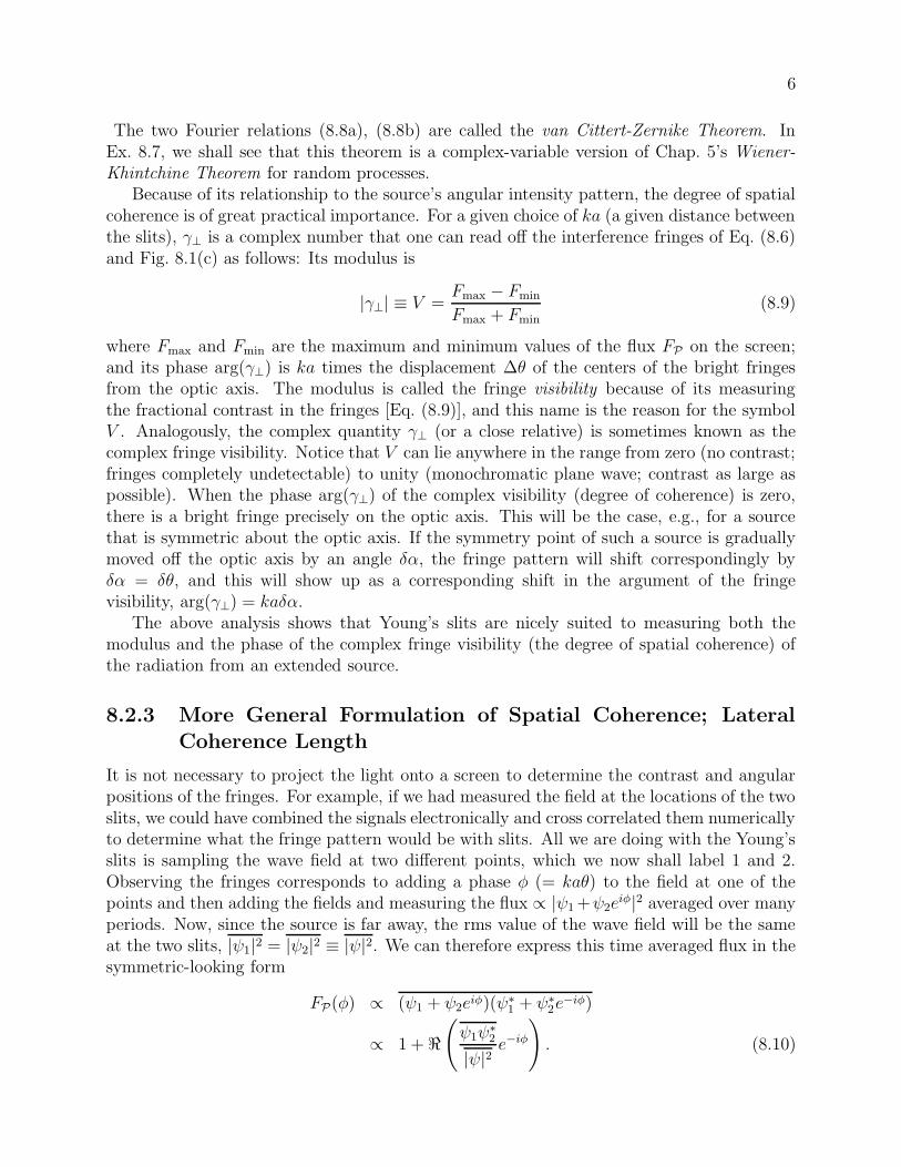
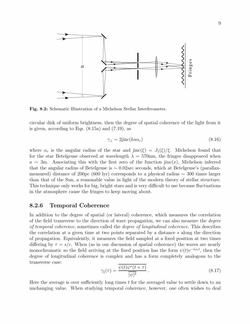
The classic implementation of Young’s slits for measuring spatial coherence is Michelson’sstellar interferometer, which Michelson used for measuring the angular diameters of Jupiter’smoons and some bright stars in 1920 and a bit earlier. The light is sampled at two smallmirrors separated by a variable distance a and then reflected onto a telescope to form in-terference fringes; cf. Fig. 8.2. (As we have emphasized, the way in which the fringes areformed is unimportant; all that matters is the two locations where the light is sampled, i.e.the first two mirrors in Fig. 8.2.) It is found that as the separation a between the mirrorsis increased, the fringe visibility V decreases. If we model a star (rather badly in fact) as a

9

a

Fri

ng

es

Fig. 8.2: Schematic Illustration of a Michelson Stellar Interferometer.

circular disk of uniform brightness, then the degree of spatial coherence of the light from itis given, according to Eqs. (8.15a) and (7.19), as

γ⊥ = 2jinc(kaαr) (8.16)

where αr is the angular radius of the star and jinc(ξ) = J1(ξ)/ξ. Michelson found thatfor the star Betelgeuse observed at wavelength λ = 570nm, the fringes disappeared whena ∼ 3m. Associating this with the first zero of the function jinc(x), Michelson inferredthat the angular radius of Betelgeuse is ∼ 0.02arc seconds, which at Betelgeuse’s (parallax-measured) distance of 200pc (600 lyr) corresponds to a physical radius ∼ 300 times largerthan that of the Sun, a reasonable value in light of the modern theory of stellar structure.This technique only works for big, bright stars and is very difficult to use because fluctuationsin the atmosphere cause the fringes to keep moving about.

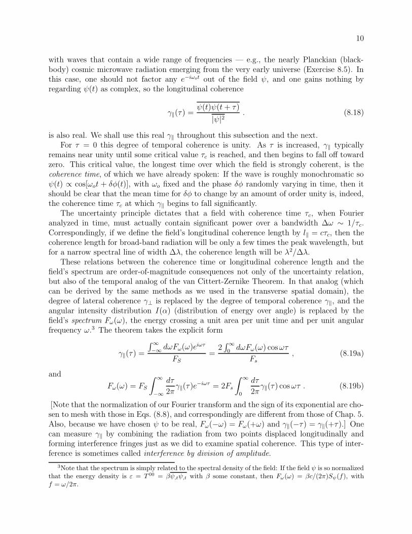
8.2.6 Temporal Coherence

In addition to the degree of spatial (or lateral) coherence, which measures the correlationof the field transverse to the direction of wave propagation, we can also measure the degreeof temporal coherence, sometimes called the degree of longitudinal coherence. This describesthe correlation at a given time at two points separated by a distance s along the directionof propagation. Equivalently, it measures the field sampled at a fixed position at two timesdiffering by τ = s/c. When (as in our discussion of spatial coherence) the waves are nearlymonochromatic so the field arriving at the fixed position has the form ψ(t)e−iωot, then thedegree of longitudinal coherence is complex and has a form completely analogous to thetransverse case:

γ‖(τ) =ψ(t)ψ∗(t+ τ)

|ψ|2. (8.17)

Here the average is over sufficiently long times t for the averaged value to settle down to anunchanging value. When studying temporal coherence, however, one often wishes to deal

10

with waves that contain a wide range of frequencies — e.g., the nearly Planckian (black-body) cosmic microwave radiation emerging from the very early universe (Exercise 8.5). Inthis case, one should not factor any e−iωot out of the field ψ, and one gains nothing byregarding ψ(t) as complex, so the longitudinal coherence

γ‖(τ) =ψ(t)ψ(t+ τ)

|ψ|2. (8.18)

is also real. We shall use this real γ‖ throughout this subsection and the next.For τ = 0 this degree of temporal coherence is unity. As τ is increased, γ‖ typically

remains near unity until some critical value τc is reached, and then begins to fall off towardzero. This critical value, the longest time over which the field is strongly coherent, is thecoherence time, of which we have already spoken: If the wave is roughly monochromatic soψ(t) ∝ cos[ωot + δφ(t)], with ωo fixed and the phase δφ randomly varying in time, then itshould be clear that the mean time for δφ to change by an amount of order unity is, indeed,the coherence time τc at which γ‖ begins to fall significantly.

The uncertainty principle dictates that a field with coherence time τc, when Fourieranalyzed in time, must actually contain significant power over a bandwidth ∆ω ∼ 1/τc.Correspondingly, if we define the field’s longitudinal coherence length by l‖ = cτc, then thecoherence length for broad-band radiation will be only a few times the peak wavelength, butfor a narrow spectral line of width ∆λ, the coherence length will be λ2/∆λ.

These relations between the coherence time or longitudinal coherence length and thefield’s spectrum are order-of-magnitude consequences not only of the uncertainty relation,but also of the temporal analog of the van Cittert-Zernike Theorem. In that analog (whichcan be derived by the same methods as we used in the transverse spatial domain), thedegree of lateral coherence γ⊥ is replaced by the degree of temporal coherence γ‖, and theangular intensity distribution I(α) (distribution of energy over angle) is replaced by thefield’s spectrum Fω(ω), the energy crossing a unit area per unit time and per unit angularfrequency ω.3 The theorem takes the explicit form

γ‖(τ) =

∫∞

−∞dωFω(ω)eiωτ

FS

=2∫∞

0dωFω(ω) cosωτ

Fs

, (8.19a)

and

Fω(ω) = FS

∫ ∞

−∞

dτ

2πγ‖(τ)e

−iωτ = 2Fs

∫ ∞

0

dτ

2πγ‖(τ) cosωτ . (8.19b)

[Note that the normalization of our Fourier transform and the sign of its exponential are cho-sen to mesh with those in Eqs. (8.8), and correspondingly are different from those of Chap. 5.Also, because we have chosen ψ to be real, Fω(−ω) = Fω(+ω) and γ‖(−τ) = γ‖(+τ).] Onecan measure γ‖ by combining the radiation from two points displaced longitudinally andforming interference fringes just as we did to examine spatial coherence. This type of inter-ference is sometimes called interference by division of amplitude.

3Note that the spectrum is simply related to the spectral density of the field: If the field ψ is so normalizedthat the energy density is ε = T 00 = βψ,tψ,t with β some constant, then Fω(ω) = βc/(2π)Sψ(f), withf = ω/2π.

11

LightSource

beam

splitt

er

InterferenceFringes

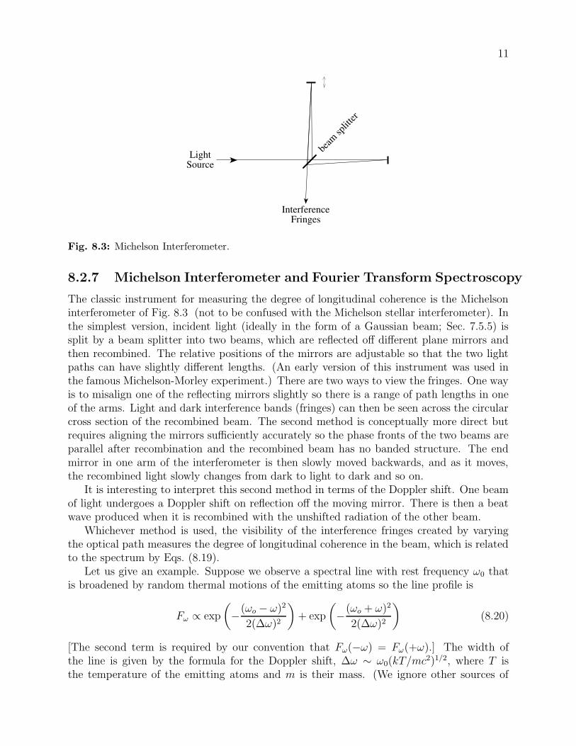
Fig. 8.3: Michelson Interferometer.

8.2.7 Michelson Interferometer and Fourier Transform Spectroscopy

The classic instrument for measuring the degree of longitudinal coherence is the Michelsoninterferometer of Fig. 8.3 (not to be confused with the Michelson stellar interferometer). Inthe simplest version, incident light (ideally in the form of a Gaussian beam; Sec. 7.5.5) issplit by a beam splitter into two beams, which are reflected off different plane mirrors andthen recombined. The relative positions of the mirrors are adjustable so that the two lightpaths can have slightly different lengths. (An early version of this instrument was used inthe famous Michelson-Morley experiment.) There are two ways to view the fringes. One wayis to misalign one of the reflecting mirrors slightly so there is a range of path lengths in oneof the arms. Light and dark interference bands (fringes) can then be seen across the circularcross section of the recombined beam. The second method is conceptually more direct butrequires aligning the mirrors sufficiently accurately so the phase fronts of the two beams areparallel after recombination and the recombined beam has no banded structure. The endmirror in one arm of the interferometer is then slowly moved backwards, and as it moves,the recombined light slowly changes from dark to light to dark and so on.

It is interesting to interpret this second method in terms of the Doppler shift. One beamof light undergoes a Doppler shift on reflection off the moving mirror. There is then a beatwave produced when it is recombined with the unshifted radiation of the other beam.

Whichever method is used, the visibility of the interference fringes created by varyingthe optical path measures the degree of longitudinal coherence in the beam, which is relatedto the spectrum by Eqs. (8.19).

Let us give an example. Suppose we observe a spectral line with rest frequency ω0 thatis broadened by random thermal motions of the emitting atoms so the line profile is

Fω ∝ exp

(

−(ωo − ω)2

2(∆ω)2

)

+ exp

(

−(ωo + ω)2

2(∆ω)2

)

(8.20)

[The second term is required by our convention that Fω(−ω) = Fω(+ω).] The width ofthe line is given by the formula for the Doppler shift, ∆ω ∼ ω0(kT/mc

2)1/2, where T isthe temperature of the emitting atoms and m is their mass. (We ignore other sources of

12

line broadening, e.g. natural broadening and pressure broadening, which actually dominateunder normal conditions.) For example with Hydrogen at 103K, ∆ω ∼ 10−5ω0.

By Fourier transforming this line profile, using the well known result that the Fouriertransform of a Gaussian is another Gaussian, and invoking the fundamental relations (8.19)between the spectrum and temporal coherence, we obtain

γ‖(τ) = exp

(

−τ2(∆ω)2

2

)

cosωoτ . (8.21)

If we had used the nearly monochromatic formalism with the field written as ψ(t)e−iωot,then we would have obtained γ‖(τ) = exp[−τ 2(∆ω)2/2]eiωoτ , the real part of which is ourbroad-band formalism’s γ‖. In either case, γ‖ oscillates with frequency ωo, and the amplitudeof this oscillation is the fringe visibility V :

V = exp

(

−τ2(∆ω)2

2

)

. (8.22)

The variation V (τ) of this visibility with lag time τ is sometimes called an interferogram.For time lags τ (∆ω)−1, the line appears to be monochromatic and fringes with unitvisibility should be seen. However for lags τ & (∆ω)−1, the fringe visibility will decreaseexponentially with τ 2. In our example, if the rest frequency is ω0 ∼ 3 × 1015rad s−1, thenthe longitudinal coherence length will be l‖ = cτc ∼ 10mm and no fringes will be seen whenthe radiation is combined from points separated by much more than this distance.

This procedure is an example of Fourier transform spectroscopy, in which, by measuringthe degree of temporal coherence γ‖(τ) and then Fourier tranforming it, one infers the shapeof the radiation’s spectrum, or in this case, the width of a specific spectral line.

When (as in Exercise 8.5) the waves are very broad band, the degree of longitudinal co-herence γ‖(τ) will not have the form of a sinusoidal oscillation (regular fringes) with slowlyvarying amplitude (visibility). Nevertheless, the van Cittert-Zernike theorem still guaran-tees that the spectrum will be the Fourier transform of the coherence γ‖(τ), which can bemeasured by a Michelson interferometer.

****************************

EXERCISES

Exercise 8.4 Problem: Longitudinal coherence of radio waves

An FM radio station has a carrier frequency of 91.3 MHz and transmits heavy metalrock music. Estimate the coherence length of the radiation.

Exercise 8.5 Problem: Cosmic Microwave Background Radiation

An example of a Michelson interferometer is the Far Infrared Absolute Spectropho-tometer (FIRAS) carried by the Cosmic Background Explorer Satellite (COBE). Oneof the goals of the COBE mission was to see if the cosmic microwave background

13

(CMB) spectrum really had the shape of 2.7K black body (Planckian) radiation, or ifit was highly distorted as some measurements made on rocket flights had suggested.The spectrophotometer used Fourier transform spectroscopy to meet this goal: it com-pared accurately the degree of longitudinal coherence γ‖ of the CMB radiation withthat of a calibrated source on board the spacecraft, which was known to be a blackbody at about 2.7K. The comparison was made by alternately feeding radiation fromthe microwave background and radiation from the calibrated source into the sameMichelson interferometer and comparing their fringe spacings. The result (Mather et.al. 1994) was that the background radiation has a spectrum that is Planckian withtemperature 2.726 ± 0.010K over the wavelength range 0.5–5 mm, in agreement withsimple cosmological theory that we shall explore in the last chapter of this book.

(a) Suppose that the CMB had had a Wien spectrum Fω ∝ |ω|3 exp(−~|ω|/kT ) whereT = 2.74K. Show that the visibility of the fringes would have been

V = |γ‖| ∝|s4 − 6s2

0s2 + s4

0|(s2 + s2

0)4

(8.23)

where s = cτ is longitudinal distance, and calculate a numerical value for s0.

(b) Compute the interferogram for a Planck function either analytically (perhaps withthe help of a computer) or numerically using a Fast Fourier Transform. Comparegraphically the interferogram for the Wien and Planck spectra.

****************************

8.2.8 Degree of Coherence; Relation to Theory of Random Pro-

cesses

Having separately discussed spatial and temporal coherence, we now can easily perform afinal generalization and define the full degree of coherence of the radiation field betweentwo points separated both laterally by a vector a and longitudinally by a distance s, orequivalently by a time τ = s/c. If we take the time-separation viewpoint, so x1 and x2 havea purely transverse spatial separation a = x2 − x1, and if we restrict ourselves to nearlymonochromatic waves and use the complex formalism of Eq. (8.13), then

γ12(ka, τ) ≡ψ(x1, t)ψ∗(x1 + a, t + τ)

[|ψ(x1, t)|2 |ψ(x1 + a, t)|2]1/2=ψ(x1, t)ψ∗(x1 + a, t + τ)

|ψ|2. (8.24)

In the second expression we have used the fact that, because the source is far away, |ψ|2is independent of the spatial location at which it is evaluated, in the region of interest.Consistent with the definition (8.24), we can define a volume of coherence as the product ofthe longitudinal coherence length l‖ = cτc and the square of the transverse coherence lengthl2⊥.

14

The three-dimensional version of the van Cittert-Zernike theorem relates the degree ofcoherence (8.24) to the radiation’s specific intensity, Iω(α, ω), i.e. to the energy crossing aunit area per unit time per unit solid angle and per unit angular frequency (energy “per uniteverything”). (Since the frequency ν and the angular frequency ω are related by ω = 2πν,the specific intensity Iω of this chapter and that Iν of Chap. 2 are related by Iν = 2πIω.)The van Cittert-Zernike theorem states that

γ12(ka, τ) =

∫

dΩαdωIω(α, ω)ei(ka·α+ωτ)

FS

, (8.25a)

and

Iω(α, ω) = FS

∫

dτd2ka

(2π)3γ12(ka, τ)e

−i(ka·α+ωτ) . (8.25b)

There obviously must be an intimate relationship between the theory of random processes,as developed in Chap. 5, and the theory of a wave’s coherence, as we have developed it inthis section, Sec. 8.2. That relationship is explained in Ex. 8.7. Most especially, it is shownthat the van Cittert-Zernike theorem is nothing but the wave’s Wiener-Khintchine theoremin disguise.

****************************

EXERCISES

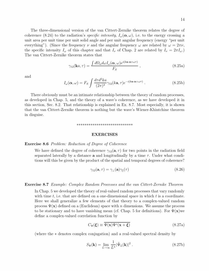
Exercise 8.6 Problem: Reduction of Degree of Coherence

We have defined the degree of coherence γ12(a, τ) for two points in the radiation fieldseparated laterally by a distance a and longitudinally by a time τ . Under what condi-tions will this be given by the product of the spatial and temporal degrees of coherence?

γ12(a, τ) = γ⊥(a)γ‖(τ) (8.26)

Exercise 8.7 Example: Complex Random Processes and the van Cittert-Zernike Theorem

In Chap. 5 we developed the theory of real-valued random processes that vary randomlywith time t, i.e. that are defined on a one-dimensional space in which t is a coordinate.Here we shall generalize a few elements of that theory to a complex-valued randomprocess Ψ(x) defined on a (Euclidean) space with n dimensions. We assume the processto be stationary and to have vanishing mean (cf. Chap. 5 for definitions). For Ψ(x)wedefine a complex-valued correlation function by

CΨ(ξ) ≡ Ψ(x)Ψ∗(x + ξ) (8.27a)

(where the ∗ denotes complex conjugation) and a real-valued spectral density by

SΨ(k) = limL→∞

1

Ln|ΨL(k)|2 . (8.27b)

15

Here ΨL is Ψ confined to a box of side L (i.e. set to zero outside that box), and thetilde denotes a Fourier transform defined using the conventions of Chap. 5:

ΨL(k) =

∫

ΨL(x)e−ik·xdnx , ΨL(x) =

∫

ΨL(k)e+ik·x dnk

(2π)n. (8.28)

Because Ψ is complex rather than real, CΨ(ξ) is complex; and as we shall see below, itscomplexity implies that [although SΨ(k) is real], SΨ(−k) 6= SΨ(k). This fact preventsus from folding negative k into positive k and thereby making SΨ(k) into a “single-sided” spectral density as we did for real random processes in Chap. 5. In this complexcase we must distinguish −k from +k and similarly −ξ from +ξ.

(a) The complex Wiener-Khintchine theorem [analog of Eqs. (5.42) and (5.43)] says that

SΨ(k) =

∫

CΨ(ξ)e+ik·ξdnξ , (8.29a)

CΨ(ξ) =

∫

SΨ(k)e−ik·ξ dnk

(2π)n. (8.29b)

Derive these relations. [Hint: use Parseval’s theorem in the form∫

A(x)B∗(x)dnx =∫

A(k)B∗(k)dnk/(2π)n with A(x) = ΨL(x) and B(x) = ΨL(x + ξ), and then takethe limit as L → ∞.] Because SΨ(k) is real, this Wiener-Khintchine theorem im-plies that CΨ(−ξ) = C∗

Ψ(ξ). Show that this is so directly from the definition (8.27a)of CΨ(ξ). Because CΨ(ξ) is complex, the Wiener-Khintchine theorem implies thatSΨ(k) 6= SΨ(−k).

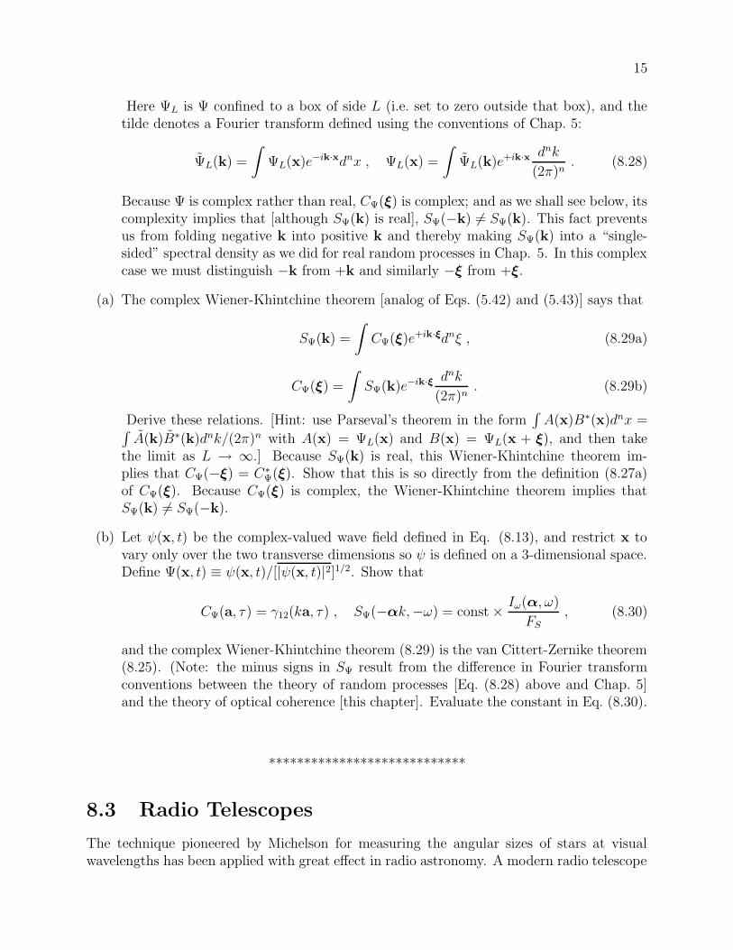
(b) Let ψ(x, t) be the complex-valued wave field defined in Eq. (8.13), and restrict x tovary only over the two transverse dimensions so ψ is defined on a 3-dimensional space.Define Ψ(x, t) ≡ ψ(x, t)/[|ψ(x, t)|2]1/2. Show that

CΨ(a, τ) = γ12(ka, τ) , SΨ(−αk,−ω) = const × Iω(α, ω)

FS, (8.30)

and the complex Wiener-Khintchine theorem (8.29) is the van Cittert-Zernike theorem(8.25). (Note: the minus signs in SΨ result from the difference in Fourier transformconventions between the theory of random processes [Eq. (8.28) above and Chap. 5]and the theory of optical coherence [this chapter]. Evaluate the constant in Eq. (8.30).

****************************

8.3 Radio Telescopes

The technique pioneered by Michelson for measuring the angular sizes of stars at visualwavelengths has been applied with great effect in radio astronomy. A modern radio telescope

16

Telescope& Amplifier

Delay Correlator

vγ (a)

v

a

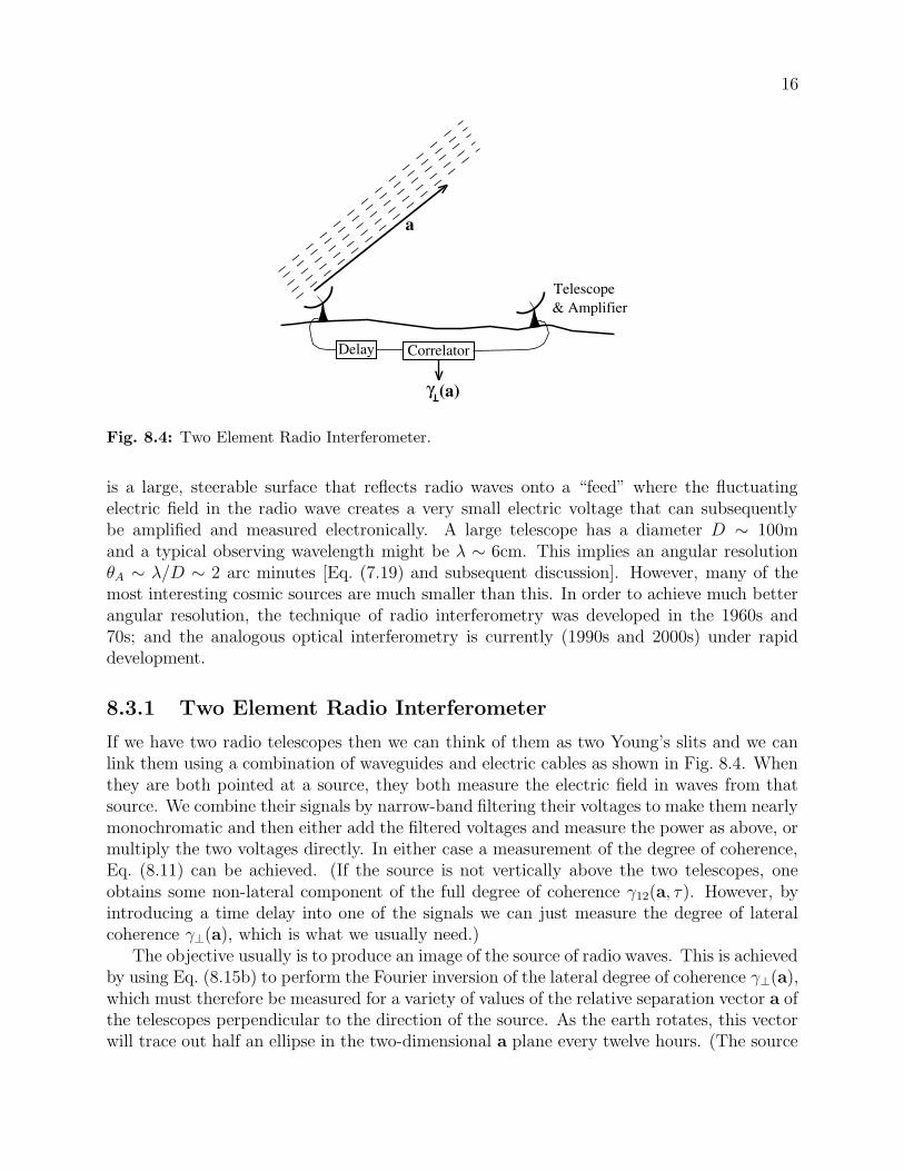
Fig. 8.4: Two Element Radio Interferometer.

is a large, steerable surface that reflects radio waves onto a “feed” where the fluctuatingelectric field in the radio wave creates a very small electric voltage that can subsequentlybe amplified and measured electronically. A large telescope has a diameter D ∼ 100mand a typical observing wavelength might be λ ∼ 6cm. This implies an angular resolutionθA ∼ λ/D ∼ 2 arc minutes [Eq. (7.19) and subsequent discussion]. However, many of themost interesting cosmic sources are much smaller than this. In order to achieve much betterangular resolution, the technique of radio interferometry was developed in the 1960s and70s; and the analogous optical interferometry is currently (1990s and 2000s) under rapiddevelopment.

8.3.1 Two Element Radio Interferometer

If we have two radio telescopes then we can think of them as two Young’s slits and we canlink them using a combination of waveguides and electric cables as shown in Fig. 8.4. Whenthey are both pointed at a source, they both measure the electric field in waves from thatsource. We combine their signals by narrow-band filtering their voltages to make them nearlymonochromatic and then either add the filtered voltages and measure the power as above, ormultiply the two voltages directly. In either case a measurement of the degree of coherence,Eq. (8.11) can be achieved. (If the source is not vertically above the two telescopes, oneobtains some non-lateral component of the full degree of coherence γ12(a, τ). However, byintroducing a time delay into one of the signals we can just measure the degree of lateralcoherence γ⊥(a), which is what we usually need.)

The objective usually is to produce an image of the source of radio waves. This is achievedby using Eq. (8.15b) to perform the Fourier inversion of the lateral degree of coherence γ⊥(a),which must therefore be measured for a variety of values of the relative separation vector a ofthe telescopes perpendicular to the direction of the source. As the earth rotates, this vectorwill trace out half an ellipse in the two-dimensional a plane every twelve hours. (The source

17

2

31

2

31

a12

a31

a23

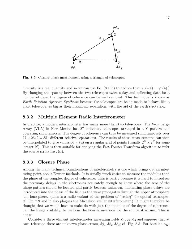
Fig. 8.5: Closure phase measurement using a triangle of telescopes.

intensity is a real quantity and so we can use Eq. (8.15b) to deduce that γ⊥(−a) = γ∗⊥(a).)By changing the spacing between the two telescopes twice a day and collecting data for anumber of days, the degree of coherence can be well sampled. This technique is known asEarth Rotation Aperture Synthesis because the telescopes are being made to behave like agiant telescope, as big as their maximum separation, with the aid of the earth’s rotation.

8.3.2 Multiple Element Radio Interferometer

In practice, a modern interferometer has many more than two telescopes. The Very LargeArray (VLA) in New Mexico has 27 individual telescopes arranged in a Y pattern andoperating simultaneosly. The degree of coherence can thus be measured simultaneously over27 × 26/2 = 351 different relative separations. The results of these measurements can thenbe interpolated to give values of γ⊥(a) on a regular grid of points (usually 2N × 2N for someinteger N). This is then suitable for applying the Fast Fourier Transform algorithm to inferthe source structure I(α).

8.3.3 Closure Phase

Among the many technical complications of interferometry is one which brings out an inter-esting point about Fourier methods. It is usually much easier to measure the modulus thanthe phase of the complex degree of coherence. This is partly because it is hard to introducethe necessary delays in the electronics accurately enough to know where the zero of thefringe pattern should be located and partly because unknown, fluctuating phase delays areintroduced into the phase of the field as the wave propagates through the upper atmosphereand ionosphere. (This is a radio variant of the problem of “seeing” for optical telescopes,cf. Ex. 7.9 and it also plagues the Michelson stellar interferometer.) It might therefore bethought that we would have to make do with just the modulus of the degree of coherence,i.e. the fringe visibility, to perform the Fourier inversion for the source structure. This isnot so.

Consider a three element interferometer measuring fields ψ1, ψ2, ψ3 and suppose that ateach telescope there are unknown phase errors, δφ1, δφ2, δφ3; cf. Fig. 8.5. For baseline a12,

18

we measure the degree of coherence γ⊥12 ∝ ψ1ψ∗2 , a complex number with phase Φ12 =

φ12 + δφ1 − δφ2, where φ12 is the phase of γ⊥12 in the absence of phase errors. If we alsomeasure the degrees of coherence for the other two pairs of telescopes in the triangle andderive their phases Φ23,Φ31, we can then calculate the quantity

C123 = Φ12 + Φ23 + Φ31

= φ12 + φ23 + φ31 (8.31)

from which the phase errors cancel out.The quantity C123, known as the closure phase, can be measured with high accuracy. In

the VLA, there are 27×26×25/6 = 2925 such closure phases, and they can all be measuredwith considerable redundancy. Although absolute phase information cannot be recovered,93 per cent of the relative phases can be inferred in this manner and used to construct animage far superior to what one would get without any phase information.

8.3.4 Angular Resolution

When the telescope spacings are well sampled and the source is bright enough to carry outthese image processing techniques, an interferometer can have an angular resolving powerapproaching that of an equivalent filled aperture as large as the maximum telescope spacing.For the VLA this is 35km, giving an angular resolution of a fraction of a second of arc at6cm wavelength, which is 350 times better than the resolution of a single 100m telescope.

Even greater angular resolution is achieved in the technique known as Very Long BaselineInterferometry (VLBI). Here the telescopes can be located on different continents and insteadof linking them directly, the oscillating field amplitudes ψ(t) are stored on magnetic tapeand then combined digitally long after the observation, to compute the complex degree ofcoherence and thence the source structure I(α). In this way angular resolutions over 300times better than those achievable by the VLA can be obtained. Structure smaller than amilliarcsecond corresponding to a few light years at cosmological distances can be measuredin this manner.

****************************

EXERCISES

Exercise 8.8 Example: Interferometry from Space

The longest radio-telescope separation currently available is that between telescopeson the earth’s surface and an 8-m diameter radio telescope in the Japanese HALCAsatellite, which orbits the earth at 6 earth radii. Radio Astronomers conventionallydescribe the specific intensity Iω(α, ω) of a source in terms of its brightness temper-ature. This is the temperature Tb(ω) that a black body would have to have in orderto emit, in the Rayleigh-Jeans (low-frequency) end of its spectrum, the same specificintensity as the source.

19

(a) Show that for a single (linear or circular) polarization, if the solid angle subtended bya source is ∆Ω and the specific flux (also called spectral flux ) measured from the sourceis Fω ≡

∫

IωdΩ = Iω∆Ω, then the brightness temperature is

Tb =2(2π)3c2IωkBω2

=2(2π)3c2Fω

kBω2∆Ω, (8.32)

where kB is Boltzmann’s constant.

(b) The brightest quasars emit radio spectral fluxes of about Fω = 10−25W m−2Hz−1,independent of frequency. The smaller is such a quasar, the larger will be its brightnesstemperature. Thus, one can characterize the smallest sources that a radio telescopesystem can resolve by the highest brightness temperatures it can measure. Show thatthe maximum brightness temperature measurable by the earth-to-orbit interferometeris independent of the frequency at which the observation is made, and estimate itsnumerical value.

****************************

8.4 Etalons and Fabry-Perot Interferometers

We have shown how a Michelson Interferometer can be used as a fourier transform spectrom-eter: one measures the complex fringe visibility as a function of the two arms’ optical pathdifference and then takes the visibility’s Fourier transform to obtain the spectrum of theradiation. The inverse process is also powerful: One can drive a Michelson interferometerwith radiation with a known, steady spectrum, and look for time variations of the positionsof its fringes caused by changes in the relative optical path lengths of the interferometer’stwo arms. This was the philosophy of the famous Michelson-Morely experiment to search forether drift, and it is also the underlying principle of a laser interferometer (“interferometric”)gravitational-wave detector.

To reach the sensitivity required for gravitational-wave detection one must to modify theMichelson interferometer by making the light travel back and forth in each arm many times.This is achieved by converting each arm into a Fabry-Perot interferometer. In this sectionwe shall study Fabry-Perot interferometers and some of their other applications, and in thenext section we shall explore their use in gravitational-wave detection.

8.4.1 Multiple Beam Interferometry; Etalons

Fabry-Perot interferometry is based on the trapping of monochromatic light between twohighly reflecting surfaces. To understand such trapping, let us consider the concrete situationwhere the reflecting surfaces are flat and parallel to each other, and the transparent mediumbetween the surfaces has one index of refraction n, while the medium on the other side of thesurfaces has another index n′. Such a device is sometimes called an etalon. One example is a

20

d

n’ n n’ n’ n n’

(a) (b)

br

t

ai

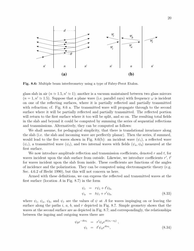
Fig. 8.6: Multiple beam interferometry using a type of Fabry-Perot Etalon.

glass slab in air (n ' 1.5, n′ ' 1); another is a vacuum maintained between two glass mirrors(n = 1, n′ ' 1.5). Suppose that a plane wave (i.e. parallel rays) with frequency ω is incidenton one of the reflecting surfaces, where it is partially reflected and partially transmittedwith refraction; cf. Fig. 8.6 a. The transmitted wave will propagate through to the secondsurface where it will be partially reflected and partially transmitted. The reflected portionwill return to the first surface where it too will be split, and so on. The resulting total fieldsin the slab and beyond it could be computed by summing the series of sequential reflectionsand transmissions. Alternatively, they can be computed as follows:

We shall assume, for pedagogical simplicity, that there is translational invariance alongthe slab (i.e. the slab and incoming wave are perflectly planar). Then the series, if summed,would lead to the five waves shown in Fig. 8.6(b): an incident wave (ψi), a reflected wave(ψr), a transmitted wave (ψt), and two internal waves with fields (ψa, ψb) measured at thefirst surface.

We now introduce amplitude reflection and transmission coefficients, denoted r and t, forwaves incident upon the slab surface from outside. Likewise, we introduce coefficients r ′, t′

for waves incident upon the slab from inside. These coefficients are functions of the anglesof incidence and the polarization. They can be computed using electromagnetic theory (e.g.Sec. 4.6.2 of Hecht 1990), but this will not concern us here.

Armed with these definitions, we can express the reflected and transmitted waves at thefirst surface (location A in Fig. 8.7) in the form

ψr = rψi + t′ψb,

ψa = tψi + r′ψb, (8.33)

where ψi, ψa, ψb, and ψr are the values of ψ at A for waves impinging on or leaving thesurface along the paths i, a, b, and r depicted in Fig. 8.7. Simple geometry shows that thewaves at the second surface are as depicted in Fig. 8.7; and correspondingly, the relationshipsbetween the ingoing and outgoing waves there are

ψbe−iks1 = r′ψae

ik(s1−s2) ,

ψt = t′ψaeiks1, (8.34)

21

b e-iks1

aeik(s1-s 2)

b

r

i

a

t

r i

a b da

A

2d tan

s2=2d tan sin s1 =

d sec

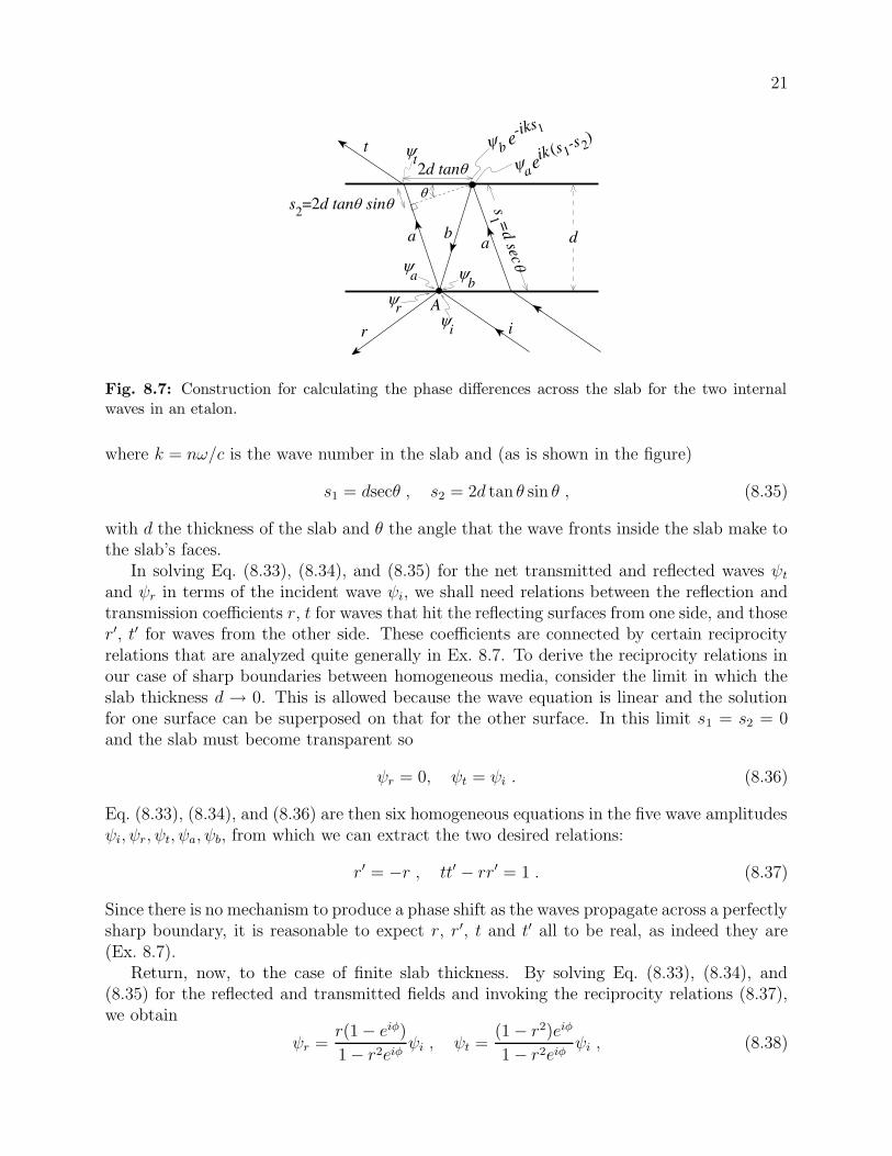
t

Fig. 8.7: Construction for calculating the phase differences across the slab for the two internalwaves in an etalon.

where k = nω/c is the wave number in the slab and (as is shown in the figure)

s1 = dsecθ , s2 = 2d tan θ sin θ , (8.35)

with d the thickness of the slab and θ the angle that the wave fronts inside the slab make tothe slab’s faces.

In solving Eq. (8.33), (8.34), and (8.35) for the net transmitted and reflected waves ψt

and ψr in terms of the incident wave ψi, we shall need relations between the reflection andtransmission coefficients r, t for waves that hit the reflecting surfaces from one side, and thoser′, t′ for waves from the other side. These coefficients are connected by certain reciprocityrelations that are analyzed quite generally in Ex. 8.7. To derive the reciprocity relations inour case of sharp boundaries between homogeneous media, consider the limit in which theslab thickness d → 0. This is allowed because the wave equation is linear and the solutionfor one surface can be superposed on that for the other surface. In this limit s1 = s2 = 0and the slab must become transparent so

ψr = 0, ψt = ψi . (8.36)

Eq. (8.33), (8.34), and (8.36) are then six homogeneous equations in the five wave amplitudesψi, ψr, ψt, ψa, ψb, from which we can extract the two desired relations:

r′ = −r , tt′ − rr′ = 1 . (8.37)

Since there is no mechanism to produce a phase shift as the waves propagate across a perfectlysharp boundary, it is reasonable to expect r, r′, t and t′ all to be real, as indeed they are(Ex. 8.7).

Return, now, to the case of finite slab thickness. By solving Eq. (8.33), (8.34), and(8.35) for the reflected and transmitted fields and invoking the reciprocity relations (8.37),we obtain

ψr =r(1 − eiφ)

1 − r2eiφψi , ψt =

(1 − r2)eiφ

1 − r2eiφψi , (8.38)

22

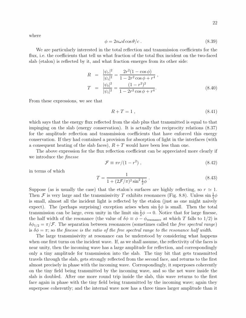
whereφ = 2nωd cos θ/c . (8.39)

We are particularly interested in the total reflection and transmission coefficients for theflux, i.e. the coefficients that tell us what fraction of the total flux incident on the two-facedslab (etalon) is reflected by it, and what fraction emerges from its other side:

R =|ψr|2|ψi|2

=2r2(1 − cosφ)

1 − 2r2 cosφ+ r4,

T =|ψt|2|ψi|2

=(1 − r2)2

1 − 2r2 cosφ+ r4. (8.40)

From these expressions, we see that

R + T = 1 , (8.41)

which says that the energy flux reflected from the slab plus that transmitted is equal to thatimpinging on the slab (energy conservation). It is actually the reciprocity relations (8.37)for the amplitude reflection and transmission coefficients that have enforced this energyconservation. If they had contained a provision for absorption of light in the interfaces (witha consequent heating of the slab faces), R + T would have been less than one.

The above expression for the flux reflection coefficient can be appreciated more clearly ifwe introduce the finesse

F ≡ πr/(1 − r2) , (8.42)

in terms of which

T =1

1 + (2F/π)2 sin2 12φ. (8.43)

Suppose (as is usually the case) that the etalon’s surfaces are highly reflecting, so r ' 1.Then F is very large and the transmissivity T exhibits resonances (Fig. 8.8). Unless sin 1

2φ

is small, almost all the incident light is reflected by the etalon (just as one might naivelyexpect). The (perhaps surprising) exception arises when sin 1

2φ is small. Then the total

transmission can be large, even unity in the limit sin 12φ → 0. Notice that for large finesse,

the half width of the resonance (the value of δφ ≡ φ − φresonance at which T falls to 1/2) isδφ1/2 = π/F . The separation between resonances (sometimes called the free spectral range)is δφ = π; so the finesse is the ratio of the free spectral range to the resonance half width.

The large transmissivity at resonance can be understood by considering what happenswhen one first turns on the incident wave. If, as we shall assume, the reflectivity of the faces isnear unity, then the incoming wave has a large amplitude for reflection, and correspondinglyonly a tiny amplitude for transmission into the slab. The tiny bit that gets transmittedtravels through the slab, gets strongly reflected from the second face, and returns to the firstalmost precisely in phase with the incoming wave. Correspondingly, it superposes coherentlyon the tiny field being transmitted by the incoming wave, and so the net wave inside theslab is doubled. After one more round trip inside the slab, this wave returns to the firstface again in phase with the tiny field being transmitted by the incoming wave; again theysuperpose coherently; and the internal wave now has a three times larger amplitude than it

23

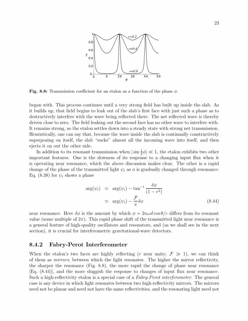
2 3 4 5

0.2

0.4

0.6

0.8

1

00 π π π ππ

φ

T

r=0.2

r=0.4

r=0.9

Fig. 8.8: Transmission coefficient for an etalon as a function of the phase φ.

began with. This process continues until a very strong field has built up inside the slab. Asit builds up, that field begins to leak out of the slab’s first face with just such a phase as todestructively interfere with the wave being reflected there. The net reflected wave is therebydriven close to zero. The field leaking out the second face has no other wave to interfere with.It remains strong, so the etalon settles down into a steady state with strong net transmission.Heuristically, one can say that, because the wave inside the slab is continually constructivelysuperposing on itself, the slab “sucks” almost all the incoming wave into itself, and thenejects it on out the other side.

In addition to its resonant transmission when | sin 12φ| 1, the etalon exhibits two other

important features. One is the slowness of its response to a changing input flux when itis operating near resonance, which the above discussion makes clear. The other is a rapidchange of the phase of the transmitted light ψt as φ is gradually changed through resonance:Eq. (8.38) for ψt shows a phase

arg(ψt) ' arg(ψi) − tan−1 δφ

(1 − r2)

' arg(ψi) −Fπδφ (8.44)

near resonance. Here δφ is the amount by which φ = 2nωd cos θ/c differs from its resonantvalue (some multiple of 2π). This rapid phase shift of the transmitted light near resonance isa general feature of high-quality oscillators and resonators, and (as we shall see in the nextsection), it is crucial for interferometric gravitational-wave detectors.

8.4.2 Fabry-Perot Interferometer

When the etalon’s two faces are highly reflecting (r near unity; F 1), we can thinkof them as mirrors, between which the light resonates. The higher the mirror reflectivity,the sharper the resonance (Fig. 8.8), the more rapid the change of phase near resonance[Eq. (8.44)], and the more sluggish the response to changes of input flux near resonance.Such a high-reflectivity etalon is a special case of a Fabry-Perot interferometer. The generalcase is any device in which light resonates between two high-reflectivity mirrors. The mirrorsneed not be planar and need not have the same reflectivities, and the resonating light need not

24

be plane fronted. For example, in an interferometric gravitational-wave detector (Fig. 8.11below) each detector arm is a Fabry-Perot cavity with spherical mirrors at its ends, themirrors have very different but high reflectivities, and the resonating light has a Gaussian-beam profile.

In the case of a Fabry-Perot etalon (parallel mirrors, plane-parallel light beam), theresonant transmission enables the etalon to be used as a spectrometer. The round-tripphase change φ = 2nωd cos θ/c inside the etalon varies linearly with the wave’s frequencyω, but only waves with phases φ near integer multiples of 2π will be transmitted efficiently.The etalon can be tuned to a particular frequency by varying either the slab width d orthe angle of incidence of the radiation (and thence the angle θ inside the etalon). Eitherway, impressively good chromatic resolving power can be achieved. We say that waves withtwo nearby frequencies can just be resolved by an etalon when the half power point of thetransmission coefficient of one wave coincides with the half power point of the transmissioncoefficient of the other. Using Eq. (8.40) we find that the phases for the two frequencies mustdiffer by δφ ∼ 2π/F ; and correspondingly, since φ = 2nωd cos θ/c, the chromatic resolvingpower is

R =λ

δλ=

2πnd

λvacδφ=

2ndFλvac

. (8.45)

Here λvac is the wavelength in vacuum — i.e. outside the etalon. If we regard the etalonas a resonant cavity, then the finesse F can be regarded as the effective quality factor Qfor the resonator. It is roughly the number of times a typical photon traverses the etalonbefore escaping. Correspondingly, the response time of the etalon on resonance, when onechanges the incoming flux, is roughly the round-trip travel time for light inside the etalon,multiplied by the finesse. Note, moreover, that as one slowly changes the round-trip phaseφ, the rate of change of the phase of the transmitted wave, d arg(ψt)/dφ, is π−1 times thefinesse [Eq. (8.44)].

8.4.3 Lasers

Fabry-Perot interferometers are exploited in the construction of many types of lasers. Forexample, in a gas phase laser, the atoms are excited to emit a spectral line. This radiationis spontaneously emitted isotropically over a wide range of frequencies. Placing the gasbetween the mirrors of a Fabry-Perot interferometer allows one or more highly collimatedand narrow-band modes to be trapped and, while trapped, to be amplified by stimulatedemission.

****************************

EXERCISES

Exercise 8.9 Example: Reciprocity Relations for a Locally Planar Optical Device

Modern mirrors, etalons, beam splitters, and other optical devices are generally madeof glass or fused silica (quartz), with dielectric coatings on their surfaces. The coatingsconsist of alternating layers of materials with different dielectric constants, so the

25

ψi eiki.x r ψi e

ikr .x

t ψi eikt .x’

ψi* e-iki.x r* ψi* e

-ikr .x

t* ψi* e-ikt .x’

(a) (b)

z

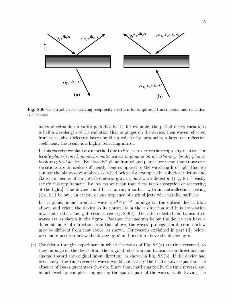
Fig. 8.9: Construction for deriving reciprocity relations for amplitude transmission and reflectioncoefficients.

index of refraction n varies periodically. If, for example, the period of n’s variationsis half a wavelength of the radiation that impinges on the device, then waves reflectedfrom successive dielectric layers build up coherently, producing a large net reflectioncoefficient; the result is a highly reflecting mirror.

In this exercise we shall use a method due to Stokes to derive the reciprocity relations forlocally plane-fronted, monochromatic waves impinging on an arbitrary, locally planar,lossless optical device. [By “locally” plane-fronted and planar, we mean that transversevariations are on scales sufficiently long compared to the wavelength of light that wecan use the plane-wave analysis sketched below; for example, the spherical mirrors andGaussian beams of an interferometric gravitational-wave detector (Fig. 8.11) easilysatisfy this requirement. By lossless we mean that there is no absorption or scatteringof the light.] The device could be a mirror, a surface with an antireflection coating(Ex. 8.11 below), an etalon, or any sequence of such objects with parallel surfaces.

Let a plane, monochromatic wave ψieiki·xe−iωt impinge on the optical device from

above, and orient the device so its normal is in the z direction and it is translationinvariant in the x and y directions; see Fig. 8.9(a). Then the reflected and transmittedwaves are as shown in the figure. Because the medium below the device can have adifferent index of refraction from that above, the waves’ propagation direction belowmay be different from that above, as shown. For reasons explained in part (d) below,we denote position below the device by x′ and position above the device by x.

(a) Consider a thought experiment in which the waves of Fig. 8.9(a) are time-reversed, sothey impinge on the device from the original reflection and transmission directions andemerge toward the original input direction, as shown in Fig. 8.9(b). If the device hadbeen lossy, the time-reversed waves would not satisfy the field’s wave equation; theabsence of losses guarantees they do. Show that, mathematically, the time reversal canbe achieved by complex conjugating the spatial part of the waves, while leaving the

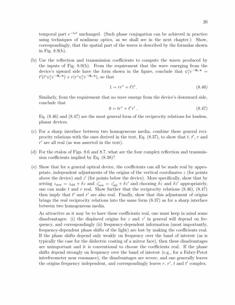
26

temporal part e−iωt unchanged. (Such phase conjugation can be achieved in practiceusing techniques of nonlinear optics, as we shall see in the next chapter.) Show,correspondingly, that the spatial part of the waves is described by the formulas shownin Fig. 8.9(b).

(b) Use the reflection and transmission coefficients to compute the waves produced bythe inputs of Fig. 8.9(b). From the requirement that the wave emerging from thedevice’s upward side have the form shown in the figure, conclude that ψ∗

i e−iki·x =

t′(t∗ψ∗i e

−iki·x) + r(r∗ψ∗i e

−iki·x), so that

1 = rr∗ + t′t∗. (8.46)

Similarly, from the requirement that no wave emerge from the device’s downward side,conclude that

0 = tr∗ + t∗r′ . (8.47)

Eq. (8.46) and (8.47) are the most general form of the reciprocity relations for lossless,planar devices.

(c) For a sharp interface between two homogeneous media, combine these general reci-procity relations with the ones derived in the text, Eq. (8.37), to show that t, t′, r andr′ are all real (as was asserted in the text).

(d) For the etalon of Figs. 8.6 and 8.7, what are the four complex reflection and transmis-sion coefficients implied by Eq. (8.38)?

(e) Show that for a general optical device, the coefficients can all be made real by appro-priate, independent adjustments of the origins of the vertical coordinates z (for pointsabove the device) and z′ (for points below the device). More specifically, show that bysetting znew = zold + δz and z′new = z′old + δz′ and choosing δz and δz′ appropriately,one can make t and r real. Show further that the reciprocity relations (8.46), (8.47)then imply that t′ and r′ are also real. Finally, show that this adjustment of originsbrings the real reciprocity relations into the same form (8.37) as for a sharp interfacebetween two homogeneous media.

As attractive as it may be to have these coefficients real, one must keep in mind somedisadvantages: (i) the displaced origins for z and z′ in general will depend on fre-quency, and correspondingly (ii) frequency-dependent information (most importantly,frequency-dependent phase shifts of the light) are lost by making the coefficients real.If the phase shifts depend only weakly on frequency over the band of interest (as istypically the case for the dielectric coating of a mirror face), then these disadvantagesare unimportant and it is conventional to choose the coefficients real. If the phaseshifts depend strongly on frequency over the band of interest (e.g., for a Fabry-Perotinterferometer near resonance), the disadvantages are severe, and one generally leavesthe origins frequency independent, and correspondingly leaves r, r′, t and t′ complex.

27

LB

T

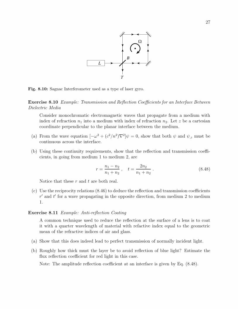
Fig. 8.10: Sagnac Interferometer used as a type of laser gyro.

Exercise 8.10 Example: Transmission and Reflection Coefficients for an Interface BetweenDielectric Media

Consider monochromatic electromagnetic waves that propagate from a medium withindex of refraction n1 into a medium with index of refraction n2. Let z be a cartesiancoordinate perpendicular to the planar interface between the medium.

(a) From the wave equation [−ω2 + (c2/n2)∇2]ψ = 0, show that both ψ and ψ,z must becontinuous across the interface.

(b) Using these continuity requirements, show that the reflection and transmission coeffi-cients, in going from medium 1 to medium 2, are

r =n1 − n2

n1 + n2, t =

2n2

n1 + n2. (8.48)

Notice that these r and t are both real.

(c) Use the reciprocity relations (8.46) to deduce the reflection and transmission coefficientsr′ and t′ for a wave propagating in the opposite direction, from medium 2 to medium1.

Exercise 8.11 Example: Anti-reflection Coating

A common technique used to reduce the reflection at the surface of a lens is to coatit with a quarter wavelength of material with refactive index equal to the geometricmean of the refractive indices of air and glass.

(a) Show that this does indeed lead to perfect transmission of normally incident light.

(b) Roughly how thick must the layer be to avoid reflection of blue light? Estimate theflux reflection coefficient for red light in this case.

Note: The amplitude reflection coefficient at an interface is given by Eq. (8.48).

28

Exercise 8.12 Problem: Sagnac Interferometer

A Sagnac interferometer is a rudimentary version of a laser gyroscope for measur-ing rotation with respect to an inertial frame. The optical configuration is shown inFig. 8.10. Light from a laser L is split by a beam splitter B and travels both clockwiseand counter-clockwise around the optical circuit, reflecting off three plane mirrors. Thelight is then combined at B and interference fringes are viewed through the telescopeT . The whole assembly rotates with angular velocity Ω.

Calculate the difference in the time it takes light to traverse the circuit in the twodirections and show that the consequent fringe shift (total number of fringes passingsome cross hairs in T ), can be expressed as ∆N = 4AΩ/cλ, where λ is the wavelengthand A is the area bounded by the beams.

****************************

8.5 Laser Interferometer Gravitational Wave Detec-

tors

As we shall discuss in Part VI, gravitational waves are predicted to exist by general relativitytheory, and their emission by a binary neutron-star system has already been monitored,via their back-action on the system’s orbital motion, at a rate consistent with the theory(leading to the award of the 1993 Nobel prize to Russell Hulse and Joseph Taylor of PrincetonUniversity). However, the gravitational analog of Hertz’s famous laboratory emission anddetection of electromagnetic waves has not yet been performed, and probably cannot bein the authors’ lifetime because of the waves’ extreme weakness. For waves strong enoughto be detectable, one must turn to violent astrophysical events, such as the collision andcoalescence of two neutron stars or black holes.

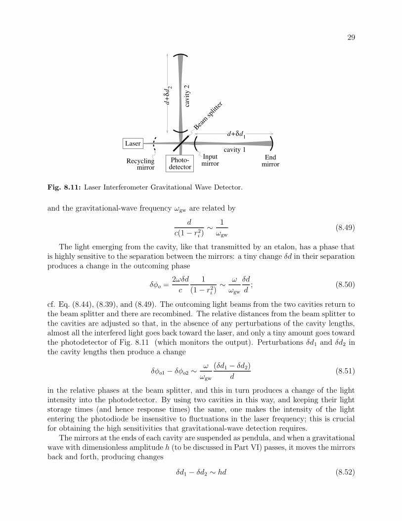
When they reach earth and pass through a laboratory, the gravitational waves shouldproduce tiny relative accelerations of free test masses. The tiny, oscillatory variation of thespacing between two such masses can be measured optically using a Michelson interferometer,in which (to increase the signal strength) each of the two arms is operated as a Fabry-Perotcavity.

The two cavities are aligned along perpendicular directions as shown in Fig. 8.11. AGaussian beam of light from a laser passes through a beam splitter, creating two beams withcorrelated phases. The beams excite the two cavities near resonance. Each cavity has an endmirror with extremely high reflectivity 1− r2

e < 10−4), and a corner mirror (“input mirror”)with a lower reflectivity, 1 − r2

i ∼ 0.01. Because of this lower reflectivity, by contrast withthe etalons discussed above, the resonant light leaks out through the input mirror instead ofthrough the end mirror. The reflectivity of the input mirror is so adjusted that the typicalphoton is stored in the cavity for roughly half the period of the expected gravitational waves(a few milliseconds), which means that the input mirror’s reflectivity r2

i , the arm length d,

29

Beam sp

litter

Endmirror

cavi

ty 2

Inputmirror

Laser

Photo-detector

cavity 1

d+d 2

δ

d+ d1δ

mirrorRecycling

Fig. 8.11: Laser Interferometer Gravitational Wave Detector.

and the gravitational-wave frequency ωgw are related by

d

c(1 − r2i )

∼ 1

ωgw(8.49)

The light emerging from the cavity, like that transmitted by an etalon, has a phase thatis highly sensitive to the separation between the mirrors: a tiny change δd in their separationproduces a change in the outcoming phase

δφo =2ωδd

c

1

(1 − r2i )

∼ ω

ωgw

δd

d; (8.50)

cf. Eq. (8.44), (8.39), and (8.49). The outcoming light beams from the two cavities return tothe beam splitter and there are recombined. The relative distances from the beam splitter tothe cavities are adjusted so that, in the absence of any perturbations of the cavity lengths,almost all the interfered light goes back toward the laser, and only a tiny amount goes towardthe photodetector of Fig. 8.11 (which monitors the output). Perturbations δd1 and δd2 inthe cavity lengths then produce a change

δφo1 − δφo2 ∼ω

ωgw

(δd1 − δd2)

d(8.51)

in the relative phases at the beam splitter, and this in turn produces a change of the lightintensity into the photodetector. By using two cavities in this way, and keeping their lightstorage times (and hence response times) the same, one makes the intensity of the lightentering the photodiode be insensitive to fluctuations in the laser frequency; this is crucialfor obtaining the high sensitivities that gravitational-wave detection requires.

The mirrors at the ends of each cavity are suspended as pendula, and when a gravitationalwave with dimensionless amplitude h (to be discussed in Part VI) passes, it moves the mirrorsback and forth, producing changes

δd1 − δd2 ∼ hd (8.52)

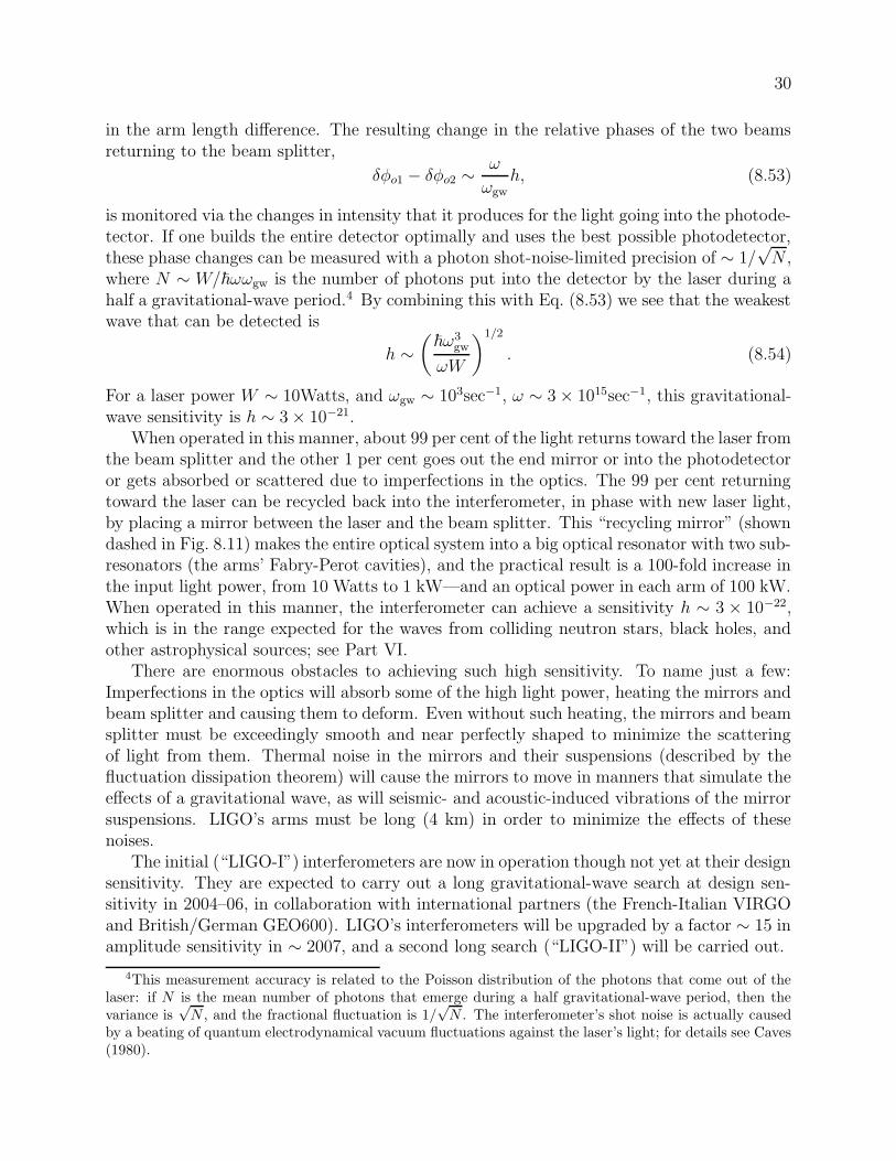
30

in the arm length difference. The resulting change in the relative phases of the two beamsreturning to the beam splitter,

δφo1 − δφo2 ∼ω

ωgwh, (8.53)

is monitored via the changes in intensity that it produces for the light going into the photode-tector. If one builds the entire detector optimally and uses the best possible photodetector,these phase changes can be measured with a photon shot-noise-limited precision of ∼ 1/

√N ,

where N ∼ W/~ωωgw is the number of photons put into the detector by the laser during ahalf a gravitational-wave period.4 By combining this with Eq. (8.53) we see that the weakestwave that can be detected is

h ∼(

~ω3gw

ωW

)1/2

. (8.54)

For a laser power W ∼ 10Watts, and ωgw ∼ 103sec−1, ω ∼ 3 × 1015sec−1, this gravitational-wave sensitivity is h ∼ 3 × 10−21.

When operated in this manner, about 99 per cent of the light returns toward the laser fromthe beam splitter and the other 1 per cent goes out the end mirror or into the photodetectoror gets absorbed or scattered due to imperfections in the optics. The 99 per cent returningtoward the laser can be recycled back into the interferometer, in phase with new laser light,by placing a mirror between the laser and the beam splitter. This “recycling mirror” (showndashed in Fig. 8.11) makes the entire optical system into a big optical resonator with two sub-resonators (the arms’ Fabry-Perot cavities), and the practical result is a 100-fold increase inthe input light power, from 10 Watts to 1 kW—and an optical power in each arm of 100 kW.When operated in this manner, the interferometer can achieve a sensitivity h ∼ 3 × 10−22,which is in the range expected for the waves from colliding neutron stars, black holes, andother astrophysical sources; see Part VI.

There are enormous obstacles to achieving such high sensitivity. To name just a few:Imperfections in the optics will absorb some of the high light power, heating the mirrors andbeam splitter and causing them to deform. Even without such heating, the mirrors and beamsplitter must be exceedingly smooth and near perfectly shaped to minimize the scatteringof light from them. Thermal noise in the mirrors and their suspensions (described by thefluctuation dissipation theorem) will cause the mirrors to move in manners that simulate theeffects of a gravitational wave, as will seismic- and acoustic-induced vibrations of the mirrorsuspensions. LIGO’s arms must be long (4 km) in order to minimize the effects of thesenoises.

The initial (“LIGO-I”) interferometers are now in operation though not yet at their designsensitivity. They are expected to carry out a long gravitational-wave search at design sen-sitivity in 2004–06, in collaboration with international partners (the French-Italian VIRGOand British/German GEO600). LIGO’s interferometers will be upgraded by a factor ∼ 15 inamplitude sensitivity in ∼ 2007, and a second long search (“LIGO-II”) will be carried out.

4This measurement accuracy is related to the Poisson distribution of the photons that come out of thelaser: if N is the mean number of photons that emerge during a half gravitational-wave period, then thevariance is

√N , and the fractional fluctuation is 1/

√N . The interferometer’s shot noise is actually caused

by a beating of quantum electrodynamical vacuum fluctuations against the laser’s light; for details see Caves(1980).

31

Photodetector

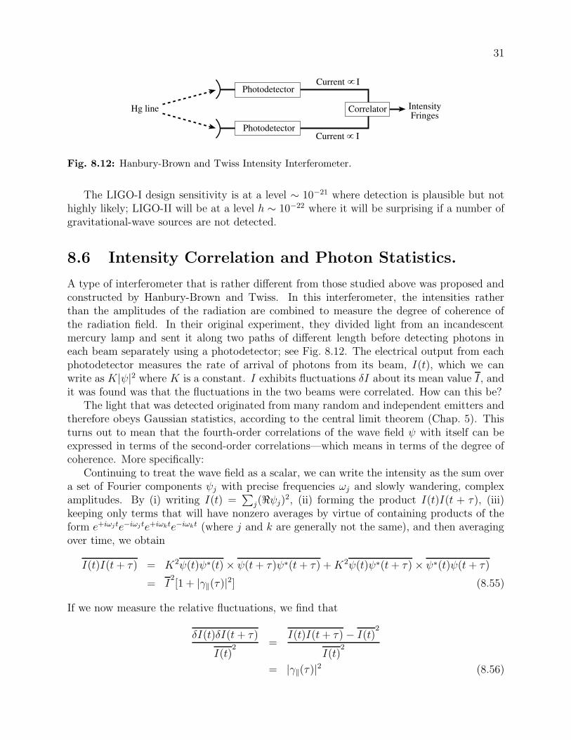
CorrelatorHg line IntensityFringes

PhotodetectorCurrent I

Current I

Fig. 8.12: Hanbury-Brown and Twiss Intensity Interferometer.

The LIGO-I design sensitivity is at a level ∼ 10−21 where detection is plausible but nothighly likely; LIGO-II will be at a level h ∼ 10−22 where it will be surprising if a number ofgravitational-wave sources are not detected.

8.6 Intensity Correlation and Photon Statistics.

A type of interferometer that is rather different from those studied above was proposed andconstructed by Hanbury-Brown and Twiss. In this interferometer, the intensities ratherthan the amplitudes of the radiation are combined to measure the degree of coherence ofthe radiation field. In their original experiment, they divided light from an incandescentmercury lamp and sent it along two paths of different length before detecting photons ineach beam separately using a photodetector; see Fig. 8.12. The electrical output from eachphotodetector measures the rate of arrival of photons from its beam, I(t), which we canwrite as K|ψ|2 where K is a constant. I exhibits fluctuations δI about its mean value I, andit was found was that the fluctuations in the two beams were correlated. How can this be?

The light that was detected originated from many random and independent emitters andtherefore obeys Gaussian statistics, according to the central limit theorem (Chap. 5). Thisturns out to mean that the fourth-order correlations of the wave field ψ with itself can beexpressed in terms of the second-order correlations—which means in terms of the degree ofcoherence. More specifically:

Continuing to treat the wave field as a scalar, we can write the intensity as the sum overa set of Fourier components ψj with precise frequencies ωj and slowly wandering, complexamplitudes. By (i) writing I(t) =

∑

j(<ψj)2, (ii) forming the product I(t)I(t + τ), (iii)

keeping only terms that will have nonzero averages by virtue of containing products of theform e+iωj te−iωj te+iωkte−iωkt (where j and k are generally not the same), and then averagingover time, we obtain

I(t)I(t+ τ) = K2ψ(t)ψ∗(t) × ψ(t+ τ)ψ∗(t+ τ) +K2ψ(t)ψ∗(t+ τ) × ψ∗(t)ψ(t+ τ)

= I2[1 + |γ‖(τ)|2] (8.55)

If we now measure the relative fluctuations, we find that

δI(t)δI(t+ τ)

I(t)2 =

I(t)I(t+ τ) − I(t)2

I(t)2

= |γ‖(τ)|2 (8.56)

32

We therefore find that the fluxes as well as the amplitudes of coherent radiation shouldexhibit positive longitudinal correlation; and the degree of coherence for the fluxes is equalto the squared modulus of the degree of coherence for the amplitudes. Although this resultwas rather controversial at the time the experiments were first performed, it is easy tointerpret qualitatively if we think in terms of photons rather then classical waves. Photonsare bosons and are therefore positively correlated even in thermal equilibrium; cf. Chaps. 2and 3. When they arrive at the beam splitter, they clump more than would be expected fora random distribution of classical particles. In fact treating the problem from the point ofview of photon statistics gives an answer equivalent to Eq. (8.56).

Some practical considerations should be mentioned. The first is that our result, Eq. (8.56)derived for a scalar wave, is really only valid for completely polarised radiation. If the incidentradiation is unpolarized, then the intensity fluctuations are reduced by a factor two. Thesecond point is that the photon counts are actually averaged over longer times than thecorrelation time of the incident radiation. This reduces the magnitude of the measuredeffect further.

Nevertheless, after successfully measuring temporal intensity correlations, Hanbury-Brownand Twiss constructed a Stellar Interferometer with which they were able to measure theangular diameters of bright stars. This method had the advantage that, as it did not dependupon the phase of the incident radiation, the results were not sensitive to atmospheric fluc-tuations, one of the drawbacks of the Michelson Stellar Interferometer. Indeed it is not evennecessary to use accurately ground mirrors to measure the effect. The method has the dis-advantage that it can only measure the modulus of the degree of coherence; the phase is lost.

****************************

EXERCISES

Exercise 8.13 Derivation: Intensity Correlations

By expressing the field as either a Fourier sum or a Fourier integral complete theargument outlined in Eq. (8.55).

Exercise 8.14 Problem: Electron Intensity Interferometry.

Is it possible to construct an intensity interferometer to measure the coherence prop-erties of an electron source? What qualitative differences do you expect there to befrom a photon intensity interferometer?

****************************

Bibliography

Caves, C. M. 1980 Quantum-mechanical radiation pressure fluctuations in an interfer-ometer Physical Review Letters 45 75

33

Feynman, R. P., Leighton, R. B., & Sands, M. 1965 The Feynman Lectures on PhysicsNew York: Addison Wesley

Francon, M. 1966 Optical Interferometry New York: Academic Press

Goodman, J. W. 1968 Introduction to Fourier Optics New York: McGraw-Hill

Hecht, E. 1998 Optics New York: Addison Wesley

Klein, M. V. & Furtak, T. E. 1986 Optics New York: Wiley

Mather, J. C. et al 1994 Measurement of the cosmic microwave background spectrumby the COBE FIRAS instrument, Astrophysical Journal 420 439

Contents

8 Interference 1

8.1 Overview . . . . . . . . . . . . . . . . . . . . . . . . . . . . . . . . . . . . . . 18.2 Coherence. . . . . . . . . . . . . . . . . . . . . . . . . . . . . . . . . . . . . . 2

8.2.1 Young’s Slits . . . . . . . . . . . . . . . . . . . . . . . . . . . . . . . 28.2.2 Interference with an Extended Source: Van Cittert-Zernike Theorem. 48.2.3 More General Formulation of Spatial Coherence; Lateral Coherence

Length . . . . . . . . . . . . . . . . . . . . . . . . . . . . . . . . . . . 68.2.4 Generalization to two dimensions . . . . . . . . . . . . . . . . . . . . 78.2.5 Michelson Stellar Interferometer . . . . . . . . . . . . . . . . . . . . . 88.2.6 Temporal Coherence . . . . . . . . . . . . . . . . . . . . . . . . . . . 98.2.7 Michelson Interferometer and Fourier Transform Spectroscopy . . . . 118.2.8 Degree of Coherence; Relation to Theory of Random Processes . . . . 13

8.3 Radio Telescopes . . . . . . . . . . . . . . . . . . . . . . . . . . . . . . . . . 158.3.1 Two Element Radio Interferometer . . . . . . . . . . . . . . . . . . . 168.3.2 Multiple Element Radio Interferometer . . . . . . . . . . . . . . . . . 178.3.3 Closure Phase . . . . . . . . . . . . . . . . . . . . . . . . . . . . . . . 178.3.4 Angular Resolution . . . . . . . . . . . . . . . . . . . . . . . . . . . . 18

8.4 Etalons and Fabry-Perot Interferometers . . . . . . . . . . . . . . . . . . . . 198.4.1 Multiple Beam Interferometry; Etalons . . . . . . . . . . . . . . . . . 198.4.2 Fabry-Perot Interferometer . . . . . . . . . . . . . . . . . . . . . . . . 238.4.3 Lasers . . . . . . . . . . . . . . . . . . . . . . . . . . . . . . . . . . . 24

8.5 Laser Interferometer Gravitational Wave Detectors . . . . . . . . . . . . . . 288.6 Intensity Correlation and Photon Statistics. . . . . . . . . . . . . . . . . . . 31

34