chapter 8 · PDF fileTechnically, goods in transit belong to the party holding legal...

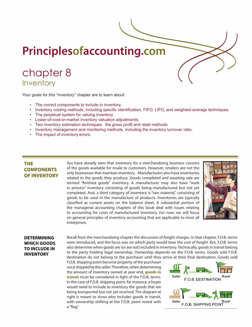
You have already seen that inventory for a merchandising business consists of the goods available for resale to customers. However, retailers are not the only businesses that maintain inventory. Manufacturers also have inventories related to the goods they produce. Goods completed and awaiting sale are termed “finished goods” inventory. A manufacturer may also have “work in process” inventory consisting of goods being manufactured but not yet completed. And, a third category of inventory is “raw material,” consisting of goods to be used in the manufacture of products. Inventories are typically classified as current assets on the balance sheet. A substantial portion of the managerial accounting chapters of this book deal with issues relating to accounting for costs of manufactured inventory. For now, we will focus on general principles of inventory accounting that are applicable to most all enterprises.

Recall from the merchandising chapter the discussion of freight charges. In that chapter, F.O.B. terms were introduced, and the focus was on which party would bear the cost of freight. But, F.O.B. terms also determine when goods are (or are not) included in inventory. Technically, goods in transit belong to the party holding legal ownership. Ownership depends on the F.O.B. terms. Goods sold F.O.B. destination do not belong to the purchaser until they arrive at their final destination. Goods sold F.O.B. shipping point become property of the purchaser once shipped by the seller. Therefore, when determining the amount of inventory owned at year end, goods in transit must be considered in light of the F.O.B. terms. In the case of F.O.B. shipping point, for instance, a buyer would need to include as inventory the goods that are being transported but not yet received. The diagram at right is meant to show who includes goods in transit, with ownership shifting at the F.O.B. point noted with a “flag.”

THE COMPONENTS OF INVENTORY

THE COMPONENTS OF INVENTORY

DETERMINING WHICH GOODS TO INCLUDE IN INVENTORY

DETERMINING WHICH GOODS TO INCLUDE IN INVENTORY

chapter 8Inventory

Principlesofaccounting.com

Your goals for this “inventory” chapter are to learn about:

The correct components to include in inventory.Inventory costing methods, including specific identification, FIFO, LIFO, and weighted-average techniques.The perpetual system for valuing inventory.Lower-of-cost-or-market inventory valuation adjustments.Two inventory estimation techniques: the gross profit and retail methods.Inventory management and monitoring methods, including the inventory turnover ratio.The impact of inventory errors.

•••••••

100 | CHAPTER 8

Another problem area pertains to goods on consignment. Consigned goods describe products that are in the custody of one party, but belong to another. Thus, the party holding physical possession is not the legal owner. The person with physical possession is known as the consignee. The consignee is responsible for taking care of the goods and trying sell them to an end customer. In essence, the consignee is acting as a sales agent. The consignor is the party holding legal ownership/title to the consigned goods in inventory. Because consigned goods belong to the consignor, they should be included in the inventory of the consignor -- not the consignee!

Consignments arise when the owner desires to place inventory in the hands of a sales agent, but the sales agent does not want to pay for those goods unless the agent is able to sell them to an end customer. For example, auto part manufacturers may produce many types of parts that are very specialized and expensive, such as braking systems. A retail auto parts store may not be able to afford to stock every variety. In addition, there is the real risk of ending up with numerous obsolete units. But, the manufacturer desperately needs these units in the retail channel -- when brakes fail, customers will go to the source that can provide an immediate solution. As a result, the manufacturer may consign the units to auto parts retailers.

Conceptually, it is fairly simple to understand the accounting for consigned goods. Practically, they pose a recordkeeping challenge. When examining a company’s inventory on hand, special care must be taken to identify both goods consigned out to others (which are to be included in inventory) and goods consigned in (which are not to be included in inventory). Obviously, if the consignee does sell the consigned goods to an end user, the consignee would keep a portion of the sales price, and remit the balance to the consignor. All of this activity requires a good accounting system to be able to identify which units are consigned, track their movement, and know when they are actually sold or returned.

Even a casual observer of the stock markets will note that stock values often move significantly on information about a company’s earnings. Now, you may be wondering why a discussion of inventory would begin with this observation. The reason is that inventory measurement bears directly on the determination of income! Recall from earlier chapters this formulation:

Notice that the goods available for sale are “allocated” to ending inventory and cost of goods sold. In the graphic, the units of inventory appear as physical units. But, in a company’s accounting records, this flow must be translated into units of money. After all, the balance sheet expresses inventory in money, not units. And, cost of goods sold on the income statement is also expressed in money:

INVENTORY COSTING METHODS

INVENTORY COSTING METHODS

InvEnToRy | 101

This means that allocating $1 less of the total cost of goods available for sale into ending inventory will necessarily result in placing $1 more into cost of goods sold (and vice versa). Further, as cost of goods sold is increased or decreased, there is an opposite effect on gross profit. Remember, sales minus cost of goods sold equals gross profit. Thus, a critical factor in determining income is the allocation of the cost of goods available for sale between ending inventory and cost of goods sold:

In earlier chapters, the dollar amount for inventory was simply given. Not much attention was given to the specific details about how that cost was determined. To delve deeper into this subject, let’s begin by considering a general rule: Inventory should include all costs that are “ordinary and necessary” to put the goods “in place” and “in condition” for their resale.

This means that inventory cost would include the invoice price, freight-in, and similar items relating to the general rule. Conversely, “carrying costs” like interest charges (if money was borrowed to buy the inventory), storage costs, and insurance on goods held awaiting sale would not be included in inventory accounts; instead those costs would be expensed as incurred. Likewise, freight-out and sales commissions would be expensed as a selling cost rather than being included with inventory.

Once the unit cost of inventory is determined via the preceding rules of logic, specific costing methods must be adopted. In other words, each unit of inventory will not have the exact same cost, and an assumption must be implemented to maintain a systematic approach to assigning costs to units on hand (and to units sold).

To solidify this point, consider a simple example: Mueller Hardware has a storage barrel full of nails. The barrel was restocked three times with 100 pounds of nails being added at each restocking. The first batch cost Mueller $100, the second batch cost Mueller $110, and the third batch cost Mueller $120. Further, the barrel was never allowed to empty completely and customers have picked all

DETERMINING THE COST OF ENDING INVENTORY

DETERMINING THE COST OF ENDING INVENTORY

COSTING METHODSCOSTING METHODS

102 | CHAPTER 8

around in the barrel as they bought nails from Mueller (and new nails were just dumped in on top of the remaining pile at each restocking). So, its hard to say exactly which nails are “physically” still in the barrel. As you might expect, some of the nails are probably from the first purchase, some from the second purchase, and some from the final purchase. Of course, they all look about the same. At the end of the accounting period, Mueller weighs the barrel and decides that 140 pounds of nails are on hand (from the 300 pounds available). The accounting question you must consider is: what is the cost of the ending inventory? Remember, this is not a trivial question, as it will bear directly on the determination of income! To deal with this very common accounting question, a company must adopt an inventory costing method (and that method must be applied consistently from year to year). The methods from which to choose are varied, generally consisting of one of the following:

First-in, first-out (FIFO)

Last-in, first-out (LIFO)

Weighted-average

Each of these methods entail certain cost-flow assumptions. Importantly, the assumptions bear no relation to the physical flow of goods; they are merely used to assign costs to inventory units. (Note: FIFO and LIFO are pronounced with a long “i” and long “o” vowel sound). Another method that will be discussed shortly is the specific identification method; as its name suggests, it does not depend on a cost flow assumption.

With first-in, first-out, the oldest cost (i.e., the first in) is matched against revenue and assigned to cost of goods sold. Conversely, the most recent purchases are assigned to units in ending inventory. For Mueller’s nails the FIFO calculations would look like this:

Last-in, first-out is just the reverse of FIFO; recent costs are assigned to goods sold while the oldest costs remain in inventory:

•

•

•

FIRST-IN, FIRST-OUT CALCULATIONS

FIRST-IN, FIRST-OUT CALCULATIONS

LAST-IN, FIRST-OUT CALCULATIONS

LAST-IN, FIRST-OUT CALCULATIONS

InvEnToRy | 103

The weighted-average method relies on average unit cost to calculate cost of units sold and ending inventory. Average cost is determined by dividing total cost of goods available for sale by total units available for sale. Mueller Hardware paid $330 for 300 pounds of nails, producing an average cost of $1.10 per pound ($330/300). The ending inventory consisted of 140 pounds, or $154. The cost of goods sold was $176 (160 pounds X $1.10):

The preceding discussion is summarized by the following comparative illustrations. Examine each, noting how the cost of beginning inventory and purchases flow to ending inventory and cost of goods sold. As you examine this drawing, you need to know that accountants usually adopt one of these cost flow assumptions to track inventory costs within the accounting system. The actual physical flow of the inventory may or may not bear a resemblance to the adopted cost flow assumption.

WEIGHTED AVERAGE CALCULATIONS

WEIGHTED AVERAGE CALCULATIONS

PRELIMINARY RECAP AND COMPARISON

PRELIMINARY RECAP AND COMPARISON

104 | CHAPTER 8

Having been introduced to the basics of FIFO, LIFO, and weighted-average, it is now time to look at a more comprehensive illustration. In this illustration, there will also be some beginning inventory that is carried over from the preceding year. Assume that Gonzales Chemical Company had a beginning inventory balance that consisted of 4,000 units with a cost of $12 per unit. Purchases and sales are shown in the schedule. The schedule suggests that Gonzales should have 5,000 units on hand at the end of the year. Assume that Gonzales conducted a physical count of inventory and confirmed that 5,000 units were actually on hand.

Based on the information in the schedule, we know that Gonzales will report sales of $304,000. This amount is the result of selling 7,000 units at $22 ($154,000) and 6,000 units at $25 ($150,000). The dollar amount of sales will be reported in the income statement, along with cost of goods sold and gross profit. How much is cost of goods sold and gross profit? The answer will depend on the cost flow assumption adopted by Gonzales.

If Gonzales uses FIFO, ending inventory and cost of goods sold calculations are as follows, producing the financial statements at right:

If Gonzales uses LIFO, ending inventory and cost of goods sold calculations are as follows, producing the financial statements at right:

DETAILED ILLUSTRATIONDETAILED ILLUSTRATION

FIFOFIFO

LIFOLIFOLIFOLIFO

Date Purchases SalesUnits on

Hand1-Jan 4,000

5-Mar 6,000 units @ $16 each 10,000

17-apr 7,000 units @ $22 each 3,000

7-sep 8,000 units @ $17 each 11,000

11-nov 6,000 units @ $25 each 5,000

Beginning inventory 4,000 X $12 = $48,000 +

net purchases ($232,000 total) 6,000 X $16 = $96,000

8,000 X $17 = $136,000

= cost of goods available for sale ($280,000 total)

4,000 X $12 = $48,000 6,000 X $16 = $96,000

8,000 X $17 = $136,000

=

ending inventory ($85,000) 5,000 X $17 = $85,000 +

cost of goods sold ($195,000 total) 4,000 X $12 = $48,000 6,000 X $16 = $96,000 3,000 X $17 = $51,000

GONZALES CHEMICAL COMPANY Income Statement

For the Year Ending December 31, 20XX

REvENuES Net sales COSt OF GOODS SOLD Beginning inventory, Jan. 1 Net purchases Goods avai lable for sale Less: Ending inventory, Dec. 31 Cost of goods sold GROSS PROFIt

. . .

$ 48,000 232,000 $280,000 85,000

$304,000

195,000 $109,000

GONZALES CHEMICAL COMPANY Balance Sheet

December 31, 20XX

ASSEtS . . .

Inventory

85,000

Beginning inventory 4,000 X $12 = $48,000 +

net purchases ($232,000 total) 6,000 X $16 = $96,000

8,000 X $17 = $136,000

= cost of goods available for sale ($280,000 total)

4,000 X $12 = $48,000 6,000 X $16 = $96,000

8,000 X $17 = $136,000

=ending inventory ($64,000)

4,000 X $12 = $48,000 1,000 X $16 = $16,000

+cost of goods sold ($216,000 total)

8,000 X $17 = $136,000 5,000 X $16 = $80,000




. . .

$ 48,000 232,000 $280,000 64,000

$304,000

216,000 $ 88,000


December 31, 20XX

ASSEtS . . .

Inventory

64,000

InvEnToRy | 105

If the company uses the weighted-average method, ending inventory and cost of goods sold calculations are as follows, producing the financial statements at right:

The following table reveals that the amount of gross profit and ending inventory numbers appear quite different, depending on the inventory method selected:

The results above are consistent with the general rule that LIFO results in the lowest income (assuming rising prices, as was evident in the Gonzales example), FIFO the highest, and weighted average an amount in between. Because LIFO tends to depress profits, you may wonder why a company would select this option; the answer is sometimes driven by income tax considerations. Lower income produces a lower tax bill, thus companies will tend to prefer the LIFO choice. Usually, financial accounting methods do not have to conform to methods chosen for tax purposes. However, in the USA, LIFO “conformity rules” generally require that LIFO be used for financial reporting if it is used for tax purposes. In many countries LIFO is not permitted for tax or accounting purposes.

Accounting theorists may argue that financial statement presentations are enhanced by LIFO because it matches recently incurred costs with the recently generated revenues. Others maintain that FIFO is better because recent costs are reported in inventory on the balance sheet. Whichever side of this debate you find yourself, it is important to note that the inventory method in use must be clearly communicated in the financial statements and related notes. Companies that use LIFO will frequently augment their reports with supplement data about what inventory would be if FIFO were instead used. No matter which method is selected, consistency in method of application should be maintained. This does not mean that changes cannot occur; however, changes should only be made if financial accounting is improved.

As was noted earlier, another inventory method is specific identification. This method requires a business to identify each unit of merchandise with the unit’s cost and retain that identification until the inventory is sold. Once a specific inventory item is sold, the cost of the unit is assigned to cost of goods sold. Specific identification requires tedious record keeping and is typically only used for inventories of uniquely identifiable goods that have a fairly high per-unit cost (e.g., automobiles, fine jewelry, and so forth).

COMPARING INVENTORY METHODS

COMPARING INVENTORY METHODS

SPECIFIC IDENTIFICATIONSPECIFIC IDENTIFICATION

cost of goods available for sale $280,000

Divided by units (4,000 + 6,000 + 8,000) 18,000

average unit cost (note: do not round) $15.5555 per unit

ending inventory (5,000 units @ $15.5555) $77,778

cost of goods sold (13,000 units @ $15.5555) $202,222




. . .

$ 48,000 232,000 $280,000 77,778

$304,000

202,222 $101,778


December 31, 20XX

ASSEtS . . .

Inventory

77,778

FIFO LIFOWeighted-

Average

sales $304,000 $304,000 $304,000

cost of Goods sold 195,000 216,000 202,222

Gross profit $109,000 $ 88,000 $101,778

ending inventory $ 85,000 $ 64,000 $ 77,778

106 | CHAPTER 8

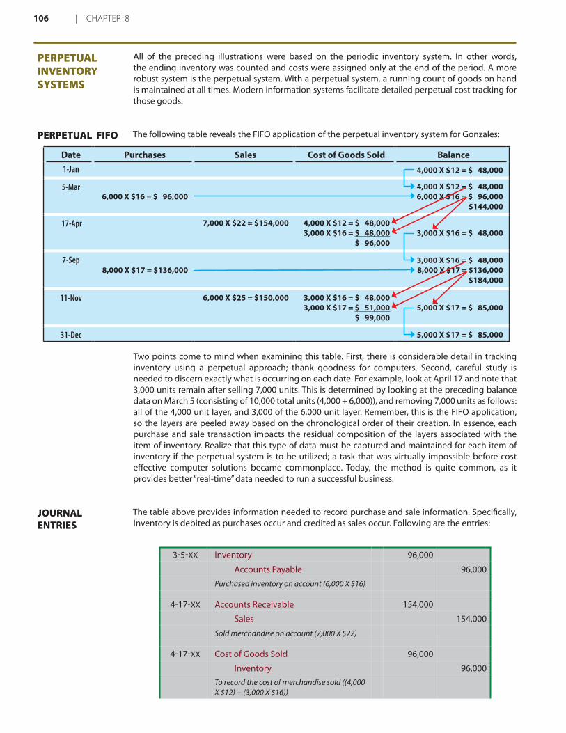
All of the preceding illustrations were based on the periodic inventory system. In other words, the ending inventory was counted and costs were assigned only at the end of the period. A more robust system is the perpetual system. With a perpetual system, a running count of goods on hand is maintained at all times. Modern information systems facilitate detailed perpetual cost tracking for those goods.

The following table reveals the FIFO application of the perpetual inventory system for Gonzales:

Two points come to mind when examining this table. First, there is considerable detail in tracking inventory using a perpetual approach; thank goodness for computers. Second, careful study is needed to discern exactly what is occurring on each date. For example, look at April 17 and note that 3,000 units remain after selling 7,000 units. This is determined by looking at the preceding balance data on March 5 (consisting of 10,000 total units (4,000 + 6,000)), and removing 7,000 units as follows: all of the 4,000 unit layer, and 3,000 of the 6,000 unit layer. Remember, this is the FIFO application, so the layers are peeled away based on the chronological order of their creation. In essence, each purchase and sale transaction impacts the residual composition of the layers associated with the item of inventory. Realize that this type of data must be captured and maintained for each item of inventory if the perpetual system is to be utilized; a task that was virtually impossible before cost effective computer solutions became commonplace. Today, the method is quite common, as it provides better “real-time” data needed to run a successful business.

The table above provides information needed to record purchase and sale information. Specifically, Inventory is debited as purchases occur and credited as sales occur. Following are the entries:

3-5-XX Inventory 96,000

Accounts Payable 96,000

Purchased inventory on account (6,000 X $16)

4-17-XX Accounts Receivable 154,000

Sales 154,000

Sold merchandise on account (7,000 X $22)

4-17-XX Cost of Goods Sold 96,000

Inventory 96,000To record the cost of merchandise sold ((4,000 X $12) + (3,000 X $16))

PERPETUAL INVENTORY SYSTEMS

PERPETUAL INVENTORY SYSTEMS

PERPETUAL FIFOPERPETUAL FIFO

JOURNAL ENTRIESJOURNAL ENTRIES

Date Purchases Sales Cost of Goods Sold Balance

1-Jan 4,000 X $12 = $ 48,000

5-Mar6,000 X $16 = $ 96,000

4,000 X $12 = $ 48,000 6,000 X $16 = $ 96,000

$144,000

17-apr 7,000 X $22 = $154,000

4,000 X $12 = $ 48,0003,000 X $16 = $ 48,000

$ 96,0003,000 X $16 = $ 48,000

7-sep8,000 X $17 = $136,000

3,000 X $16 = $ 48,000 8,000 X $17 = $136,000

$184,000

11-nov 6,000 X $25 = $150,000

3,000 X $16 = $ 48,000 3,000 X $17 = $ 51,000

$ 99,0005,000 X $17 = $ 85,000

31-Dec 5,000 X $17 = $ 85,000

InvEnToRy | 107

9-7-XX Inventory 136,000

Accounts Payable 136,000

Purchased inventory on account (8,000 X $17)

11-11-XX Accounts Receivable 150,000

Sales 150,000

Sold merchandise on account (6,000 X $25)

11-11-XX Cost of Goods Sold 99,000

Inventory 99,000To record the cost of merchandise sold ((3,000 X $16) + (3,000 X $17))

Let’s see how these entries impact certain ledger accounts and the resulting financial statements:

If you are very perceptive, you will note that this is the same thing that resulted under the periodic FIFO approach introduced earlier. So, another general observation is in order: The FIFO method will produce the same financial statement results no matter whether it is applied on a periodic or perpetual basis. This occurs because the beginning inventory and early purchases are peeled away and charged to cost of goods sold -- whether the associated calculations are done “as you go” (perpetual) or “at the end of the period” (periodic).

Account: Inventory

Date Description Debit credit Balance

Jan. 1, 20XX Balance forward $ 48,000

Mar. 5, 20XX Purchase transaction $ 96,000 144,000

Apr. 17, 20XX Sale transaction $ 96,000 48,000

Sept. 7, 20XX Purchase transaction 136,000 184,000

Nov. 11, 20XX Sale transaction 99,000 85,000

Account: Sales


Jan. 1, 20XX Balance forward $ -

Apr. 17, 20XX Sale transaction $154,000 154,000


Account: cost of goods sold



Apr. 17, 20XX Sale transaction $ 96,000 96,000


GONZALES CHEMICAL COMPANY

Income StatementFor the Year Ending December 31, 20XX

Net sales Cost of goods sold Gross prof i t Expenses

$304,000 195,000 $109,000

. . .


December 31, 20XXAssets . . .

Inventory

85,000

108 | CHAPTER 8

LIFO can also be applied on a perpetual basis. This time, the results will not be the same as the periodic LIFO approach (because the “last-in” layers are constantly being peeled away, rather than waiting until the end of the period). The following table reveals the application of a perpetual LIFO approach. Study it carefully, this time noting that sales transactions result in a peeling away of the most recent purchase layers. The journal entries are not repeated here for the LIFO approach. Do note, however, that the accounts would be the same (as with FIFO); only the amounts would change.

PERPETUAL LIFOPERPETUAL LIFO


1-Jan 4,000 X $12 = $ 48,000

5-Mar6,000 X $16 = $ 96,000

4,000 X $12 = $ 48,000 6,000 X $16 = $ 96,000

$144,000

17-apr 7,000 X $22 = $154,000

6,000 X $16 = $ 96,0001,000 X $12 = $ 12,000

$108,0003,000 X $12 = $ 36,000

7-sep8,000 X $17 = $136,000

3,000 X $12 = $ 36,000 8,000 X $17 = $136,000

$172,000

11-nov 6,000 X $25 = $150,000

6,000 X $17 = $102,000

3,000 X $12 = $ 36,000 2,000 X $17 = $ 34,000

$ 70,000

31-Dec 3,000 X $12 = $ 36,000 2,000 X $17 = $ 34,000

$ 70,000


1-Jan 4,000 X $12 = $ 48,000

5-Mar6,000 X $16 = $ 96,000

4,000 X $12 = $ 48,000 6,000 X $16 = $ 96,000

$144,000

17-apr 7,000 X $22 = $154,000

6,000 X $16 = $ 96,0001,000 X $12 = $ 12,000

$108,0003,000 X $12 = $ 36,000

7-sep8,000 X $17 = $136,000

3,000 X $12 = $ 36,000 8,000 X $17 = $136,000

$172,000

11-nov 6,000 X $25 = $150,000

6,000 X $17 = $102,000

3,000 X $12 = $ 36,000 2,000 X $17 = $ 34,000

$ 70,000

31-Dec 3,000 X $12 = $ 36,000 2,000 X $17 = $ 34,000

$ 70,000

Account: Inventory







Account: Sales













$304,000 210,000 $ 94,000

. . .



Inventory

70,000

InvEnToRy | 109

The average method can also be applied on a perpetual basis, earning it the name “moving average” approach. This technique is considerably more involved, as a new average unit cost must be computed with each purchase transaction. For the last time, we will look at the Gonzales Chemical Company data:

The resulting financial data using the moving-average approach are:

As with the periodic system, observe that the perpetual system produced the lowest gross profit via LIFO, the highest with FIFO, and the moving-average fell in between.

MOVING AVERAGEMOVING AVERAGE


1-Jan 4,000 X $12 = $ 48,000

5-Mar6,000 X $16 = $ 96,000

4,000 X $12 = $ 48,000 6,000 X $16 = $ 96,000

$144,000

17-apr 7,000 X $22 = $154,000 7,000 X $14.40 = $100,800 3,000 X $14.40 = $ 43,200

7-sep8,000 X $17 = $136,000

3,000 X $14.40 = $ 43,200 8,000 X $17 = $136,000

$179,200

11-nov 6,000 X $25 = $150,000 6,000 X $16.2909 = $97,745 5,000 X $16.2909 = $ 81,455

31-Dec 5,000 X $16.2909 = $ 81,455

$144,000/10,000 units

$14.40 per unit

$179,200/11,000 units $16.2909 per unit

Account: Inventory







Account: Sales













$304,000 198,545 $ 94,000

. . .



Inventory

81,455

110 | CHAPTER 8

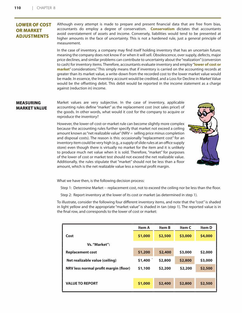
Although every attempt is made to prepare and present financial data that are free from bias, accountants do employ a degree of conservatism. Conservatism dictates that accountants avoid overstatement of assets and income. Conversely, liabilities would tend to be presented at higher amounts in the face of uncertainty. This is not a hardened rule, just a general principle of measurement.

In the case of inventory, a company may find itself holding inventory that has an uncertain future; meaning the company does not know if or when it will sell. Obsolescence, over supply, defects, major price declines, and similar problems can contribute to uncertainty about the “realization” (conversion to cash) for inventory items. Therefore, accountants evaluate inventory and employ “lower of cost or market” considerations.” This simply means that if inventory is carried on the accounting records at greater than its market value, a write-down from the recorded cost to the lower market value would be made. In essence, the Inventory account would be credited, and a Loss for Decline in Market Value would be the offsetting debit. This debit would be reported in the income statement as a charge against (reduction in) income.

Market values are very subjective. In the case of inventory, applicable accounting rules define “market” as the replacement cost (not sales price!) of the goods. In other words, what would it cost for the company to acquire or reproduce the inventory?

However, the lower-of-cost-or-market rule can become slightly more complex because the accounting rules further specify that market not exceed a ceiling amount known as “net realizable value” (NRV = selling price minus completion and disposal costs). The reason is this: occasionally “replacement cost” for an inventory item could be very high (e.g., a supply of slide rules at an office supply store) even though there is virtually no market for the item and it is unlikely to produce much net value when it is sold. Therefore, “market” for purposes of the lower of cost or market test should not exceed the net realizable value. Additionally, the rules stipulate that “market” should not be less than a floor amount, which is the net realizable value less a normal profit margin.

What we have then, is the following decision process:

Step 1: Determine Market -- replacement cost, not to exceed the ceiling nor be less than the floor.

Step 2: Report inventory at the lower of its cost or market (as determined in step 1).

To illustrate, consider the following four different inventory items, and note that the “cost” is shaded in light yellow and the appropriate “market value” is shaded in tan (step 1). The reported value is in the final row, and corresponds to the lower of cost or market:

LOWER OF COST OR MARKET ADJUSTMENTS

LOWER OF COST OR MARKET ADJUSTMENTS

MEASURING MARKET VALUEMEASURING MARKET VALUE

Item A Item B Item C Item D

Cost $1,000 $2,500 $3,000 $4,000

Vs. “Market”:

Replacement cost $1,200 $2,400 $3,000 $2,000

Net realizable value (ceiling) $1,400 $2,800 $2,800 $3,000

NRV less normal profit margin (floor) $1,100 $2,200 $2,200 $2,500

VALUE TO REPORT $1,000 $2,400 $2,800 $2,500

InvEnToRy | 111

Despite the apparent focus on detail, it is noteworthy that the lower of cost or market adjustments can be made for each item in inventory, or for the aggregate of all the inventory. In the latter case, the good offsets the bad, and a write-down is only needed if the overall market is less than the overall cost. In any event, once a write-down is deemed necessary, the loss should be recognized in income and inventory should be reduced. Once reduced, the Inventory account becomes the new basis for valuation and reporting purposes going forward. Write-ups of previous write-downs (e.g., if slide rules were to once again become hot selling items and experience a recovery in value) would not be permitted under GAAP.

Whether a company uses a periodic or perpetual inventory system, a physical count of goods on hand should occur from time to time. The quantities determined via the physical count are presumed to be correct, and any differences between the physical count and amounts reflected in the accounting records should be matched with an adjustment to the accounting records. Sometimes, however, a physical count may not be possible or is not cost effective. Then, estimation methods are employed.

One such estimation technique is the gross profit method. This method might be used to estimate inventory on hand for purposes of preparing monthly or quarterly financial statements, and certainly would come into play if a fire or other catastrophe destroyed the inventory. Such estimates are often used by insurance companies to establish the amount that has been lost by an insured party. Very simply, a company’s historical normal gross profit rate (i.e., gross profit as a percentage of sales) would be used to estimate the amount of gross profit and cost of sales. Once these data are known, it is relatively simple to project the lost inventory.

For example, assume that Tiki’s inventory was destroyed by fire. Sales for the year, prior to the date of the fire were $1,000,000, and Tiki usually sells goods at a 40% gross profit rate. Therefore, Tiki can readily estimate that cost of goods sold was $600,000. Tiki’s beginning of year inventory was $500,000, and $800,000 in purchases had occurred prior to the date of the fire. The inventory destroyed by fire can be estimated via the gross profit method, as shown.

A method that is widely used by merchandising firms to value or estimate ending inventory is the retail method. This method would only work where a category of inventory sold at retail has a consistent mark-up. The cost-to-retail percentage is multiplied times ending inventory at retail. Ending inventory at retail can be determined by a physical count of goods on hand, at their retail value. Or, sales might be subtracted from goods available for sale at retail. This option is shown in the following example.

To illustrate, Crock Buster, a specialty cookware store, sells pots that cost $7.50 for $10 -- yielding a cost to retail percentage of 75%. The beginning inventory totaled $200,000 (at cost), purchases were $300,000 (at cost), and sales totaled $460,000 (at retail). The calculations suggest an ending inventory that has a cost of $155,000. In reviewing these calculations,

APPLICATION OF THE LOWER-OF-COST-OR-MARKET RULE

APPLICATION OF THE LOWER-OF-COST-OR-MARKET RULE

INVENTORY ESTIMATION TECHNIQUES

INVENTORY ESTIMATION TECHNIQUES

GROSS PROFIT METHODGROSS PROFIT METHOD

RETAIL METHODRETAIL METHOD

112 | CHAPTER 8

note that the only “givens” are circled in yellow. These three data points are manipulated by the cost to retail percentage to solve for several unknowns. Be careful to note the percentage factor is divided within the red arrows and multiplied within the blue.

The best run companies will minimize their investment in inventory. Inventory is costly and involves the potential for loss and spoilage. In the alternative, being out of stock may result in lost customers, so a delicate balance must be maintained. Careful attention must be paid to the inventory levels. One ratio that is often used to monitor inventory is the Inventory Turnover Ratio. This ratio shows the number of times that a firm’s inventory balance was turned (“sold”) during a year. It is calculated by dividing cost of sales by the average inventory level:

Inventory Turnover Ratio =

Cost of Goods Sold/Average Inventory

If a company’s average inventory was $1,000,000, and the annual cost of goods sold was $8,000,000, you would deduce that inventory turned over 8 times (approximately once every 45 days). This could be good or bad depending on the particular business; if the company was a baker it would be very bad news, but a lumber yard might view this as good. So, general assessments are not in order. What is important is to monitor the turnover against other companies in the same line of business, and against prior years’ results for the same company. A declining turnover rate might indicate poor management, slow moving goods, or a worsening economy. In making such comparisons and evaluations, you should now be clever enough to recognize that the choice of inventory method affects the reported amounts for cost of goods sold and average inventory. As a result, the impacts of the inventory method in use must be considered in any analysis of inventory turnover ratios.

In the process of maintaining inventory records and the physical count of goods on hand, errors may occur. It is quite easy to overlook goods on hand, count goods twice, or simply make mathematical mistakes. Therefore, it is vital that accountants and business owners fully understand the effects of inventory errors and grasp the need to be careful to get these numbers as correct as possible.

A general rule is that overstatements of ending inventory cause over-statements of income, while understatements of ending inventory cause understatements of income. For instance, compare the following correct and incorrect scenario -- where the only difference is an overstatement of ending inventory by $1,000 (note that purchases were correctly recorded -- if they had not, the general rule of thumb would not hold):

INVENTORY MANAGEMENTINVENTORY MANAGEMENT

INVENTORY ERRORSINVENTORY ERRORS

InvEnToRy | 113

Had the above inventory error been an understatement ($3,000 instead of the correct $4,000), then the ripple effect would have caused an understatement of income by $1,000.

Inventory errors tend to be counterbalancing. That is, one year’s ending inventory error becomes the next year’s beginning inventory error. The general rule of thumb is that overstatements of beginning inventory cause that year’s income to be understated, while understatements of beginning inventory cause overstatements of income. Examine the following table where the only error relates to beginning inventory balances:

Hence, if the above data related to two consecutive years, the total income would be correct ($13,000 + $13,000 = $14,000 + $12,000). However, the amount for each year is critically flawed.

Correct Incorrect

Beginning inventory $ 4,000 $ 5,000

Purchases 11,000 11,000

Cost of goods available for sale $15,000 $16,000

Ending inventory 3,000 3,000

Cost of goods sold $12,000 $13,000

Sales $25,000 $25,000

Cost of goods sold 12,000 13,000

Gross profit $13,000 $12,000

Correct Incorrect


Purchases 11,000 11,000




Sales $25,000 $25,000


Gross profit $13,000 $12,000

overstateD

unDerstates

Correct Incorrect


Purchases 11,000 11,000




Sales $25,000 $25,000


Gross profit $13,000 $14,000

overstateD

overstates

114 | CHAPTER 8

chapter 8 · PDF fileTechnically, goods in transit belong to the party holding legal...

Documents

Transcript of chapter 8 · PDF fileTechnically, goods in transit belong to the party holding legal...