Chapter 8 Cluster analysis - Laboratoire de Pierre...
48
Chapter 8 Cluster analysis 8.0 A search for discontinuities Humans have always tried to classify the animate and inanimate objects that surround them. Classifying objects into collective categories is a prerequisite to naming them. It requires the recognition of discontinuous subsets in an environment which is sometimes discrete, but most often continuous. To cluster is to recognize that objects are sufficiently similar to be put in the same group and to also identify distinctions or separations between groups. Measures of similarity between objects (Q mode) or descriptors (R mode) have been discussed in Chapter 7. The present Chapter considers the different criteria that may be used to decide whether objects are similar enough to be allocated to a group; it also shows that different clustering strategies correspond to different definitions of a what a cluster is. Few ecological theories predict the existence of discontinuities in nature. Evolutionary theory tells taxonomists that discontinuities exist between species, which are the basic units of evolution, as a result of reproductive barriers; taxonomists use classification methods to reveal these discontinuities. For the opposite reason, taxonomists are not surprised to find continuous differentiation at the sub-species level. In contrast, the world that ecologists try to understand is most often a continuum. In numerical ecology, methods used to identify clusters must therefore be more contrasting than in numerical taxonomy. Ecologists who have applied taxonomic clustering methods directly to data, without first considering the theoretical applicability of such methods, have often obtained disappointing results. This has led many ecologists to abandon clustering methods altogether, hence neglecting the rich potential of similarity measures, described in Chapter 7, and to rely instead on factor analysis and other ordination methods. These are not always adapted to ecological data and, in any case, they don’t aim at bringing out partitions, but gradients. Given a sufficiently large group of objects, ecological clustering methods should be able to recognize clusters of similar objects while ignoring the few intermediates which often persist between clusters. Indeed, one cannot expect to find discontinuities when clustering sampling sites unless the physical environment is itself discontinuous,
Transcript of Chapter 8 Cluster analysis - Laboratoire de Pierre...
Chapter
8 Cluster analysis
8.0 A search for discontinuities
Humans have always tried to classify the animate and inanimate objects that surroundthem. Classifying objects into collective categories is a prerequisite to naming them. Itrequires the recognition of discontinuous subsets in an environment which issometimes discrete, but most often continuous.
To cluster is to recognize that objects are sufficiently similar to be put in the samegroup and to also identify distinctions or separations between groups. Measures ofsimilarity between objects (Q mode) or descriptors (R mode) have been discussed inChapter 7. The present Chapter considers the different criteria that may be used todecide whether objects are similar enough to be allocated to a group; it also shows thatdifferent clustering strategies correspond to different definitions of a what a cluster is.
Few ecological theories predict the existence of discontinuities in nature.Evolutionary theory tells taxonomists that discontinuities exist between species, whichare the basic units of evolution, as a result of reproductive barriers; taxonomists useclassification methods to reveal these discontinuities. For the opposite reason,taxonomists are not surprised to find continuous differentiation at the sub-specieslevel. In contrast, the world that ecologists try to understand is most often a continuum.In numerical ecology, methods used to identify clusters must therefore be morecontrasting than in numerical taxonomy. Ecologists who have applied taxonomicclustering methods directly to data, without first considering the theoreticalapplicability of such methods, have often obtained disappointing results. This has ledmany ecologists to abandon clustering methods altogether, hence neglecting the richpotential of similarity measures, described in Chapter 7, and to rely instead on factoranalysis and other ordination methods. These are not always adapted to ecological dataand, in any case, they don’t aim at bringing out partitions, but gradients.
Given a sufficiently large group of objects, ecological clustering methods should beable to recognize clusters of similar objects while ignoring the few intermediateswhich often persist between clusters. Indeed, one cannot expect to find discontinuitieswhen clustering sampling sites unless the physical environment is itself discontinuous,

304 Cluster analysis
or unless sampling occurred at opposite ends of a gradient, instead of within thegradient (Whittaker, 1962: 88). Similarly, when looking for associations of species,small groups of densely associated species are usually found, with the other speciesgravitating around one or more of the association nuclei.
The result of clustering ecological objects sampled from a continuum is oftencalled a typology (i.e. a system of types). In such a case, the purpose of clustering is toidentify various object types which may be used to describe the structure of thecontinuum; it is thus immaterial to wonder whether these clusters are “natural” orunique.
For readers with no practical experience in clustering, Section 8.2 provides adetailed account of single linkage clustering, which is simple to understand and is usedto introduce the principles of clustering. The review of other methods includes asurvey of the main dichotomies among existing methods (Section 8.4), followed by adiscussion of the most widely available methods of interest to ecologists (8.5, 8.7 and8.8). Theoretical aspects are discussed in Sections 8.3 and 8.6. Section 8.9 deals withclustering algorithms useful in identifying biological associations, whereasSection 8.10 gives an overview of seriation, a method useful to cluster non-symmetricresemblance matrices. A review of clustering statistics, methods of cluster validation,and graphical representations, completes the chapter (Sections 8.11 to 8.13). Therelationships between clustering and other steps of data analysis are depicted inFig. 10.3.
Several, but not all statistical packages offer clustering capabilities. All packageswith clustering procedures offer at least a Lance & Williams algorithm capable ofcarrying out the clustering methods listed in Table 8.8. Many also have a K-meanspartitioning algorithm. Few offer proportional-link linkage or additional forms ofclustering. Some methods are available in specialized packages only: clustering withconstraints of temporal (Section 12.6) or spatial contiguity (Section 13.3); fuzzyclustering (e.g. Bezdek, 1987); or clustering by neural network algorithms(e.g. Fausett, 1994). The main difference among packages lies in the list ofresemblance coefficients available (Section 7.7). Ecologists should consider this pointwhen selecting a clustering package.
While most packages nowadays illustrate clustering results in the form ofdendrograms, some programs use “skyline plots”, which are also called “trees” or“icicle plots”. These plots contain the same information as dendrograms but are ratherodd to read and interpret. The way to transform a skyline plot into a dendrogram isexplained in Section 8.13.
Despite the versatility of clustering methods, one should remember that not allproblems are clustering problems. Before engaging in clustering, one should be able tojustify why one believes that discontinuities exist in the data; or else, explain that onehas a practical need to divide a continuous swarm of objects into groups.
Typology
Definitions 305
8.1 Definitions
Clustering is an operation of multidimensional analysis which consists in partitioningthe collection of objects (or descriptors) in the study. A partition (Table 8.1) is adivision of a set (collection) into subsets, such that each object or descriptor belongs toone and only one subset for that partition (Legendre & Rogers, 1972). Theclassification of objects (or descriptors) that results from clustering may include asingle partition, or several hierarchically nested partitions of the objects (ordescriptors), depending on the clustering model that has been selected.
From this definition, it follows that the subsets of any level of partition form aseries of mutually exclusive cells, among which the objects (or descriptors) aredistributed. This definition a priori excludes all classification models in which classeshave elements in common (overlapping clusters) or in which objects have fractionaldegrees of membership in different clusters (fuzzy partitions: Bezdek, 1987); thesemodels have not been used in ecology yet. This limitation is such that a “hard” or“crisp” (versus fuzzy) partition has the same definition as a descriptor (Section 1.4).Each object is characterized by a state (its cluster) of the classification and it belongs toonly one of the clusters. This property will be useful for the interpretation ofclassifications (Chapter 10), since any partition may be considered as a qualitativedescriptor and compared as such to any other descriptor. A clustering of objectsdefined in this way imposes a discontinuous structure onto the data set, even if theobjects have originally been sampled from a continuum. This structure results from thegrouping into subsets of objects that are sufficiently similar, given the variablesconsidered, and from the observation that different subsets possess uniquerecognizable characteristics.
ClusteringPartition
Table 8.1 Example of hierarchically nested partitions of a group of objects (e.g. sampling sites). The firstpartition separates the objects by the environment to which they belong. The second partition,hierarchically nested into the first, recognizes clusters of sites in each of the two environments.
Partition 1 Partition 2 Sampling sites
Cluster 1 7, 12
Observations in environment A Cluster 2 3, 5, 11
Cluster 3 1, 2, 6
Cluster 4 4, 9Observations in environment B
Cluster 5 8, 10, 13, 14
306 Cluster analysis
Clustering has been part of ecological tradition for a long time. It goes back to thePolish ecologist Kulczynski (1928), who needed to cluster ecological observations; hedeveloped a method quite remote from the clustering algorithms discussed in theparagraphs to come. His technique, called seriation, consists in permuting the rows andcolumns of an association matrix in such a way as to maximize the values on thediagonal. The method is still used in phytosociology, anthropology, social sciences,and other fields; it is described in Section 8.10 where an analytical solution to theproblem is presented.
Most clustering (this Chapter) and ordination (Chapter 9) methods proceed fromassociation matrices (Chapter 7). Distinguishing between clustering and ordination issomewhat recent. While ordination in reduced space goes back to Spearman (factoranalysis: 1904), most modern clustering methods have only been developed since theera of second-generation computers. The first programmed method, developed forbiological purposes, goes back to 1958 (Sokal & Michener)*. Before that, one simplyplotted the objects in a scatter diagram with respect to a few variables or principalaxes; clusters were then delineated manually (Fig. 8.1) following a method whichtoday would be called centroid (Section 8.4), based upon the Euclidean distancesamong points. This empirical clustering method still remains the best approach whenthe number of variables is small and the structure to be delineated is not obscured byintermediate objects between clusters.
Clustering is a family of techniques which is undergoing rapid development. Intheir report on the literature they reviewed, Blashfield & Aldenderfer (1978)mentioned that they found 25 papers in 1964 that contained references to the basictexts on clustering; they found 136 papers in 1970, 294 in 1973, and 501 in 1976. Thenumber has been growing ever since. Nowadays, hundreds of mathematicians andresearchers from various application fields are collaborating within 10 national ormultinational Classification Societies throughout the world, under the umbrella of theInternational Federation of Classification Societies founded in 1985.
The commonly-used clustering methods are based on easy-to-understandmathematical constructs: arithmetic, geometric, graph-theoretic, or simple statisticalmodels (minimizing within-group variance), leading to rather simple calculations onthe similarity or dissimilarity values. It must be understood that most clusteringmethods are heuristic; they create groups by reference to some concept of what a groupembedded in some space should be like, but without reference, in most case, to theprocesses occurring in the application field — ecology in the present book. They havebeen developed first by the schools of numerical taxonomists and numericalecologists, later joined by other researchers in the physical sciences and humanities.
* Historical note provided by Prof. F. James Rohlf: “Actually, Sokal & Michener (1958) did notuse a computer for their very large study. They used an electromechanical accounting machineto compute the raw sums and sums of products. The coefficients of correlation and the clusteranalysis itself were computed by hand with the use of mechanical desk calculators. Sneath diduse a computer in his first study.”
Definitions 307
Clusters are delineated on the basis of statements such as: “x1 is closer to x2 than it isto x3”, whereas other methods rest on probabilistic models of the type: “Chances arehigher that x1 and x2 pertain to the same group than x1 and x3”. In all cases, clusteringmodels make it possible to link the points without requiring prior positioning in agraph (i.e. a metric space), which would be impractical in more than three dimensions.These models thus allow a graphical representation of other interesting relationshipsamong the objects in the data set, for example the dendrogram of theirinterrelationships. Chapter 10 will show how it is possible to combine clustering andordination, computed with different methods, to obtain a more complete picture of thedata structure.
The choice of a clustering method is as critical as the choice of an associationmeasure. It is important to fully understand the properties of clustering methods inorder to correctly interpret the ecological structure they bring out. Most of all, themethods to be used depend upon the type of clustering sought. Williams et al. (1971)recognized two major categories of methods. In a descriptive clustering,misclassifying objects is to be avoided, even at the expense of creating single objectclusters. In a synoptic clustering, all objects are forced into one of the main clusters;the objective is to construct a general conceptual model which encompasses a realitywider than the data under study. Both approaches are useful.
Figure 8.1 Empirically delineating clusters of objects in a scatter diagram is easy when there are nointermediate objects between the groups.
Descriptor 2
Descriptor 1
Descriptive,synopticclustering

308 Cluster analysis
When two or more clustering models seem appropriate to a problem, ecologistsshould apply them all to the data and compare the results. Clusters that repeatedlycome out of all runs (based on appropriate methods) are the robust solutions to theclustering problem. Differences among results must be interpreted in the light of theknown properties of clustering models, which are explained in the following sections.
8.2 The basic model: single linkage clustering
For natural scientists, a simple-to-understand clustering method (or model) is singlelinkage (or nearest neighbour) clustering (Sneath, 1957). Its logic seems natural, sothat it is used to introduce readers to the principles of clustering. Its name, singlelinkage, distinguishes it from other clustering models, called complete or intermediatelinkage, detailed in Section 8.4. The algorithm for single linkage clustering issequential, agglomerative, and hierarchical, following the nomenclature ofSection 8.3. Its starting point is any association matrix (similarity or distance) amongthe objects or descriptors to be clustered. One assumes that the association measurehas been carefully chosen, following the recommendations of Section 7.6. To simplifythe discussion, the following will deal only with objects, although the method isequally applicable to an association matrix among descriptors.
The method proceeds in two steps:
• First, the association matrix is rewritten in order of decreasing similarities (orincreasing distances), heading the list with the two most similar objects of theassociation matrix, followed by the second most similar pair, and proceeding until allthe measures comprised in the association matrix have been listed.
• Second, the clusters are formed hierarchically, starting with the two most similarobjects, and then letting the objects clump into groups, and the groups aggregate to oneanother, as the similarity criterion is relaxed. The following example illustrates thismethod.
Ecological application 8.2
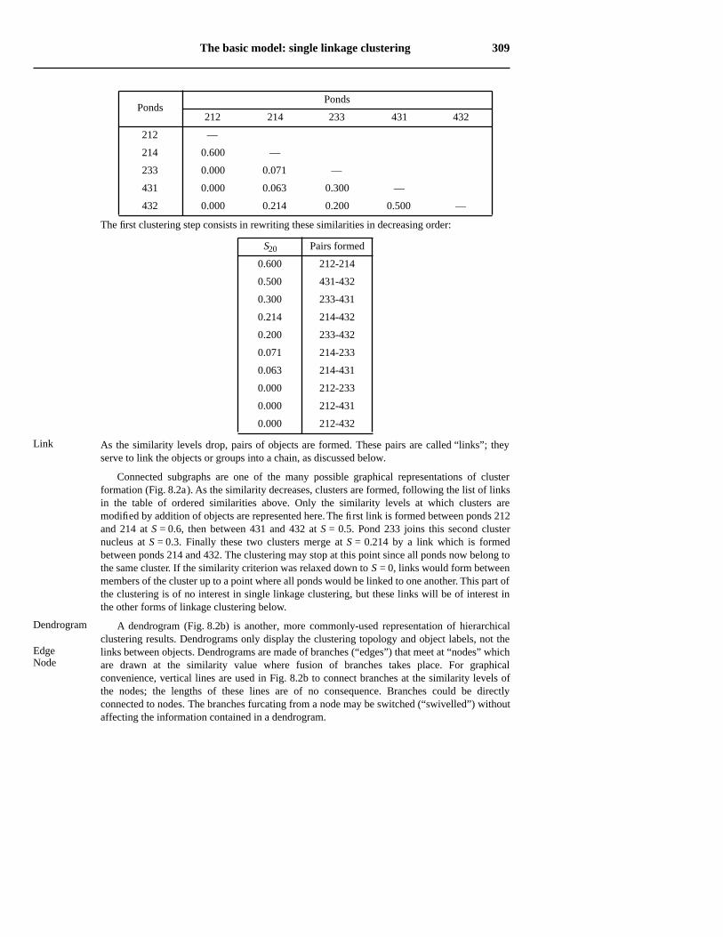
Five ponds characterized by 38 zooplankton species have been studied by Legendre &Chodorowski (1977). The data were counts, recorded on a relative abundance scale from0 = absent to 5 = very abundant. These ponds have already been used as example for thecomputation of Goodall’s coefficient (S23, Chapter 7; only eight zooplankton species were usedin that example). These five ponds, with others, have been subjected to single linkage clusteringafter computing similarity coefficient S20 with parameter k = 2. The symmetric similarity matrixis represented by its lower triangle. The diagonal is trivial because it contains 1’s by construct.
The basic model: single linkage clustering 309
The first clustering step consists in rewriting these similarities in decreasing order:
As the similarity levels drop, pairs of objects are formed. These pairs are called “links”; theyserve to link the objects or groups into a chain, as discussed below.
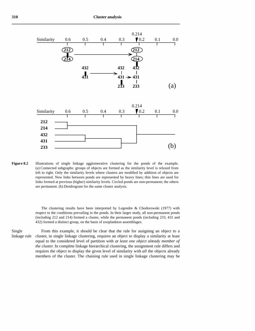
Connected subgraphs are one of the many possible graphical representations of clusterformation (Fig. 8.2a). As the similarity decreases, clusters are formed, following the list of linksin the table of ordered similarities above. Only the similarity levels at which clusters aremodified by addition of objects are represented here. The first link is formed between ponds 212and 214 at S = 0.6, then between 431 and 432 at S = 0.5. Pond 233 joins this second clusternucleus at S = 0.3. Finally these two clusters merge at S = 0.214 by a link which is formedbetween ponds 214 and 432. The clustering may stop at this point since all ponds now belong tothe same cluster. If the similarity criterion was relaxed down to S = 0, links would form betweenmembers of the cluster up to a point where all ponds would be linked to one another. This part ofthe clustering is of no interest in single linkage clustering, but these links will be of interest inthe other forms of linkage clustering below.
A dendrogram (Fig. 8.2b) is another, more commonly-used representation of hierarchicalclustering results. Dendrograms only display the clustering topology and object labels, not thelinks between objects. Dendrograms are made of branches (“edges”) that meet at “nodes” whichare drawn at the similarity value where fusion of branches takes place. For graphicalconvenience, vertical lines are used in Fig. 8.2b to connect branches at the similarity levels ofthe nodes; the lengths of these lines are of no consequence. Branches could be directlyconnected to nodes. The branches furcating from a node may be switched (“swivelled”) withoutaffecting the information contained in a dendrogram.
PondsPonds
212 214 233 431 432
212 —
214 0.600 —
233 0.000 0.071 —
431 0.000 0.063 0.300 —
432 0.000 0.214 0.200 0.500 —
S20 Pairs formed
0.600 212-214
0.500 431-432
0.300 233-431
0.214 214-432
0.200 233-432
0.071 214-233
0.063 214-431
0.000 212-233
0.000 212-431
0.000 212-432
Link
Dendrogram
EdgeNode
310 Cluster analysis
The clustering results have been interpreted by Legendre & Chodorowski (1977) withrespect to the conditions prevailing in the ponds. In their larger study, all non-permanent ponds(including 212 and 214) formed a cluster, while the permanent ponds (including 233, 431 and432) formed a distinct group, on the basis of zooplankton assemblages.
From this example, it should be clear that the rule for assigning an object to acluster, in single linkage clustering, requires an object to display a similarity at leastequal to the considered level of partition with at least one object already member ofthe cluster. In complete linkage hierarchical clustering, the assignment rule differs andrequires the object to display the given level of similarity with all the objects alreadymembers of the cluster. The chaining rule used in single linkage clustering may be
Figure 8.2 Illustrations of single linkage agglomerative clustering for the ponds of the example.(a) Connected subgraphs: groups of objects are formed as the similarity level is relaxed fromleft to right. Only the similarity levels where clusters are modified by addition of objects arerepresented. New links between ponds are represented by heavy lines; thin lines are used forlinks formed at previous (higher) similarity levels. Circled ponds are non-permanent; the othersare permanent. (b) Dendrogram for the same cluster analysis.
Similarity 0.6 0.5 0.4 0.3 0.1 0.0
212214
233
0.2140.2
(b)431432
Similarity 0.6 0.5 0.4 0.3 0.1 0.0
212
214
431
432
0.2140.2
233
431
432
212
214
(a)233
431
432
Singlelinkage rule
The basic model: single linkage clustering 311
stated as follows: at each level of partition, two objects must be allocated to the samesubset if their degree of similarity is equal to or higher than that of the partitioninglevel considered. The same rule can be formulated in terms of dissimilarities(distances) instead: two objects must be allocated to the same subset if theirdissimilarity is less than or equal to that of the partitioning level considered.
Estabrook (1966) discussed single linkage clustering using the language of graph theory.The exercise has didactic value. A cluster is defined through the following steps:
a) For any pair of objects x1 and x2, a link is defined between them by a relation Gc :
x1 Gc x2 if and only if S(x1, x2) ≥ c
or equally, if D (x1, x2) ≤ (1 – c)
Index c in clustering relation Gc is the similarity level considered. At a similarity level of 0.55,for instance, ponds 212 and 214 of the example are in relation G0.55 since S(212, 214) ≥ 0.55.This definition of a link has the properties of symmetry (x1 Gc x2 if and only if x2 Gc x1) andreflexivity (xi Gc xi is always true since S(xi, xi) = 1.0). A group of links for a set of objects,such as defined by relation Gc, is called an undirected graph.
b) The chaining which characterizes single linkage clustering may be described by a Gc-chain. AGc-chain is said to extend from x1 to x2 if there exist other points x3, x4, …, xi in the collectionof objects under study, such that x1 Gc x3 and x3 Gc x4 and … and xi Gc x2. For instance, atsimilarity level c = 0.214 of the example, there exists a G0.214-chain from pond 212 to pond 233,since there are intermediate ponds such that 212 G0.214 214 and 214 G0.214 432 and432 G0.214 431 and 431 G0.214 233. The number of links in a Gc-chain defines theconnectedness of a cluster (Subsection 8.11.1).
c) There only remains to delineate the clusters resulting from single linkage chaining. For thatpurpose, an equivalence relation Rc (“member of the same cluster”) is defined as follows:
x1 Rc x2 if and only if there exists a Gc-chain from x1 to x2 at similarity level c.
In other words, x1 and x2 are assigned to the same cluster at similarity level c if there exists achain of links joining x1 to x2. Thus, at level S = 0.214 in the example, ponds 212 and 233 areassigned to the same cluster (212 R0.214 233) because there exists a G0.214-chain from 212 to233. The relationship “member of the same cluster” has the following properties: (1) it isreflexive (xi Rc xi) because Gc is reflexive; (2) the Gc-chains may be reversed because Gc issymmetric; as a consequence, x1 Rc x2 implies that x2 Rc x1; and (3) it is transitive because, byGc-chaining, x1 Rc x2 and x2 Rc x3 implies that x1 Rc x3. Each cluster thus defined is a connectedsubgraph, which means that the objects of a cluster are all connected in their subgraph; in thegraph of all the objects, distinct clusters (subgraphs) have no links attaching them to one another.
Single linkage clustering provides an accurate picture of the relationships betweenpairs of objects but, because of its propensity to chaining, it may be undesirable forecological analysis. This means that the presence of an object midway between twocompact clusters, or a few intermediates connecting the two clusters, is enough to turnthem into a single cluster. Of course, clusters do not chain unless intermediates arepresent; so, the occurrence of chaining provides information about the data. To
Link
Undirectedgraph
ChainChaining
Connectedsubgraph
312 Cluster analysis
describe this phenomenon, Lance & Williams (1967c) wrote that this method contractsthe reference space. Picture the objects as laying in A-space (Fig. 7.2). The presence ofa cluster increases the probability of inclusion, by chaining, of neighbouring objectsinto the cluster. This is as if the distances between objects were smaller in that regionof the space; see also Fig. 8.23a.
Section 10.1 will show how to take advantage of the interesting properties of singlelinkage clustering by combining it with ordination results, while avoiding the undueinfluence of chaining on the clustering structure.
Ecologists who have access to several computer programs for single linkageclustering should rely on those that permit recognition of the first connection makingan object a member of a cluster, or allowing two clusters to fuse. These similaritiesform a chain of primary (Legendre, 1976) or external connections (Legendre &Rogers, 1972), also called dendrites by Lukaszewicz (1951). They are very usefulwhen analysing clusters drawn in an ordination space (Section 10.1). Dendrites arealso called a network (Prim, 1957), a Prim network (Cavalli-Sforza & Edwards, 1967),a minimum spanning tree (Gower & Ross, 1969), a shortest spanning tree, or aminimum-length tree (Sneath & Sokal, 1973). If these dendrites are drawn on a scatterdiagram of the objects, one can obtain a non-hierarchical clustering of the objects byremoving the last (weakest) similarity links. Such graphs are illustrated in Figs. 10.1and 10.2, drawn on top of an ordination in a space of principal coordinates; they mayalso be drawn without any reference space.
8.3 Cophenetic matrix and ultrametric property
Any classification or partition can be fully described by a cophenetic matrix. Thismatrix is used for comparing different classifications of the same objects.
1 — Cophenetic matrix
The cophenetic similarity (or distance) of two objects x1 and x2 is defined as thesimilarity (or distance) level at which objects x1 and x2 become members of the samecluster during the course of clustering (Jain & Dubes, 1988), as depicted by connectedsubgraphs or a dendrogram (Fig. 2a, b). Any dendrogram can be uniquely representedby a matrix in which the similarity (or distance) for a pair of objects is their copheneticsimilarity (or distance). Consider the single linkage clustering dendrogram of Fig. 8.2.The clustering levels, read directly on the dendrogram, lead to the following matricesof similarity (S) and distance (D, where D = 1 – S):
Chain ofprimaryconnections
Minimumspanningtree
Copheneticsimilarity
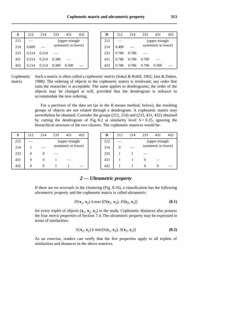
Cophenetic matrix and ultrametric property 313
Such a matrix is often called a cophenetic matrix (Sokal & Rohlf, 1962; Jain & Dubes,1988). The ordering of objects in the cophenetic matrix is irrelevant; any order thatsuits the researcher is acceptable. The same applies to dendrograms; the order of theobjects may be changed at will, provided that the dendrogram is redrawn toaccommodate the new ordering.
For a partition of the data set (as in the K-means method, below), the resultinggroups of objects are not related through a dendrogram. A cophenetic matrix maynevertheless be obtained. Consider the groups (212, 214) and (233, 431, 432) obtainedby cutting the dendrogram of Fig. 8.2 at similarity level S = 0.25, ignoring thehierarchical structure of the two clusters. The cophenetic matrices would be:
2 — Ultrametric property
If there are no reversals in the clustering (Fig. 8.16), a classification has the followingultrametric property and the cophenetic matrix is called ultrametric:
D(x1, x2) ≤ max [D(x1, x3), D(x2, x3)] (8.1)
for every triplet of objects (x1, x2, x3) in the study. Cophenetic distances also possessthe four metric properties of Section 7.4. The ultrametric property may be expressed interms of similarities:
S (x1, x2) ≥ min[S (x1, x3), S(x2, x3)] (8.2)
As an exercise, readers can verify that the five properties apply to all triplets ofsimilarities and distances in the above matrices.
S 212 214 233 431 432 D 212 214 233 431 432
212 — (upper triangle symmetric to lower)
212 — (upper triangle symmetric to lower)214 0.600 — 214 0.400 —
233 0.214 0.214 — 233 0.786 0.786 —
431 0.214 0.214 0.300 — 431 0.786 0.786 0.700 —
432 0.214 0.214 0.300 0.500 — 432 0.786 0.786 0.700 0.500 —
S 212 214 233 431 432 D 212 214 233 431 432
212 — (upper triangle symmetric to lower)
212 — (upper triangle symmetric to lower)214 1 — 214 0 —
233 0 0 — 233 1 1 —
431 0 0 1 — 431 1 1 0 —
432 0 0 1 1 — 432 1 1 0 0 —
Copheneticmatrix
314 Cluster analysis
8.4 The panoply of methods
Clustering algorithms have been developed using a wide range of conceptual modelsand for studying a variety of problems. Sneath & Sokal (1973) propose a classificationof clustering procedures. Its main dichotomies are now briefly described.
1 — Sequential versus simultaneous algorithms
Most clustering algorithms are sequential in the sense that they proceed by applying arecurrent sequence of operations to the objects. The agglomerative single linkageclustering of Section 8.2 is an example of a sequential method: the search for theequivalence relation Rc is repeated at all levels of similarity in the association matrix,up to the point where all objects are in the same cluster. In simultaneous algorithms,which are less frequent, the solution is obtained in a single step. Ordination techniques(Chapter 9), which may be used for delineating clusters, are of the latter type. This isalso the case of the direct complete linkage clustering method presented in Section 8.9.The K-means (Section 8.8) and other non-hierarchical partitioning methods may becomputed using sequential algorithms, although these methods are neitheragglomerative nor divisive (next paragraph).
2 — Agglomeration versus division
Among the sequential algorithms, agglomerative procedures begin with thediscontinuous partition of all objects, i.e. the objects are considered as being separatefrom one another. They are successively grouped into larger and larger clusters until asingle, all-encompassing cluster is obtained. If the continuous partition of all objects isused instead as the starting point of the procedure (i.e. a single group containing allobjects), divisive algorithms subdivide the group into sub-clusters, and so on until thediscontinuous partition is reached. In either case, it is left to users to decide which ofthe intermediate partitions is to be retained, given the problem under study.Agglomerative algorithms are the most developed for two reasons. First, they areeasier to program. Second, in clustering by division, the erroneous allocation of anobject to a cluster at the beginning of the procedure cannot be corrected afterwards(Gower, 1967) unless a special procedure is embedded in the algorithm to do so.
3 — Monothetic versus polythetic methods
Divisive clustering methods may be monothetic or polythetic. Monothetic models usea single descriptor as basis for partitioning, whereas polythetic models use severaldescriptors which, in most cases, are combined into an association matrix (Chapter 7)prior to clustering. Divisive monothetic methods proceed by choosing, for eachpartitioning level, the descriptor considered to be the best for that level; objects arethen partitioned following the state to which they belong with respect to thatdescriptor. For example, the most appropriate descriptor at each partitioning levelcould be the one that best represents the information contained in all other descriptors,
The panoply of methods 315
after measuring the reciprocal information between descriptors (Subsection 8.6.1).When a single partition of the objects is sought, monothetic methods produce theclustering in a single step.
4 — Hierarchical versus non-hierarchical methods
In hierarchical methods, the members of inferior-ranking clusters become members oflarger, higher-ranking clusters. Most of the time, hierarchical methods produce non-overlapping clusters, but this is not a necessity according to the definition of“hierarchy” in the dictionary or the usage recognized by Sneath & Sokal (1973).Single linkage clustering of Section 8.2 and the methods of Sections 8.5 and 8.6 arehierarchical. Non-hierarchical methods are very useful in ecology. They produce asingle partition which optimizes within-group homogeneity, instead of a hierarchicalseries of partitions optimizing the hierarchical attribution of objects to clusters. Lance& Williams (1967d) restrict the term “clustering” to the non-hierarchical methods andcall the hierarchical methods “classification”. Non-hierarchical methods include K-means partitioning, the ordination techniques (Chapter 9) used as clustering methods,the primary connection diagrams (dendrites) between objects with or without areference space, the methods of similarity matrix seriation of Section 8.10, and one ofthe algorithms of Section 8.9 for the clustering of species into biological associations.These methods should be used in cases where the aim is to obtain a directrepresentation of the relationships among objects instead of a summary of theirhierarchy. Hierarchical methods are easier to compute and more often available instatistical data analysis packages than non-hierarchical procedures.
Most hierarchical methods use a resemblance matrix as their starting point. Thisprevents their use with very large data sets because the resemblance matrix, with itsn (n – 1)/2 values, becomes extremely large and may exceed the handling capacity ofcomputers. Jambu & Lebeaux (1983) have described a fast algorithm for thehierarchical agglomeration of very large numbers of objects (e.g. n = 5000). Thisalgorithm computes a fraction only of the n (n – 1)/2 distance values. Rohlf (1978,1982a) has also developed a rather complex algorithm allowing one to obtain singlelinkage clustering after computing only a small fraction of the distances.
5 — Probabilistic versus non-probabilistic methods
Probabilistic methods include the clustering model of Clifford & Goodall (1967) andthe parametric and nonparametric methods for estimating density functions inmultivariate space.
In the method of Clifford & Goodall (1967), clusters are formed in such a way thatthe within-group association matrices have a given probability of being homogeneous.This clustering method is discussed at length in Subsection 8.9.2, where it isrecommended, in conjunction with Goodall's similarity coefficient (S23, Chapter 7),for the clustering of species into biological associations.

316 Cluster analysis
Sneath & Sokal (1973) describe other dichotomies for clustering methods, whichare of lesser interest to ecologists. These are: global or local criteria, direct or iterativesolutions, equal or unequal weights, and adaptive or non-adaptive clustering.
8.5 Hierarchical agglomerative clustering
Most methods of hierarchical agglomeration can be computed as special cases of ageneral model which is discussed in Subsection 8.5.9.
1 — Single linkage agglomerative clustering
In single linkage agglomeration (Section 8.2), two clusters fuse when the two objectsclosest to each other (one in each cluster) reach the similarity of the consideredpartition. (See also the method of simultaneous single linkage clustering described inSubsection 8.9.1). As a consequence of chaining, results of single linkage clusteringare sensitive to noise in the data (Milligan, 1996), because noise changes the similarityvalues and may thus easily modify the order in which objects cluster. The origin ofsingle linkage clustering is found in a collective work by Florek, Lukaszewicz, Perkal,Steinhaus, and Zubrzycki, published by Lukaszewicz in 1951.
2 — Complete linkage agglomerative clustering
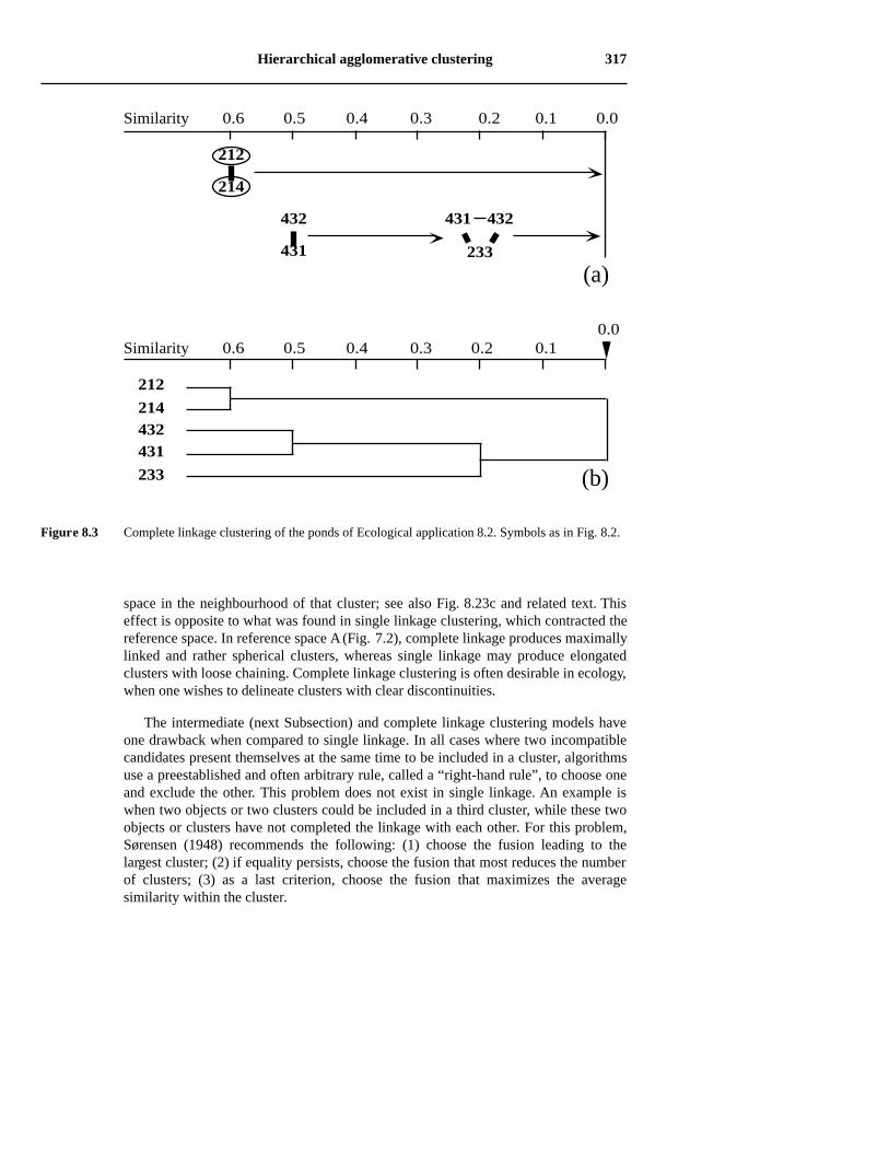
Opposite to the single linkage approach is complete linkage agglomeration , also calledfurthest neighbour sorting. In this method, first proposed by Sørensen (1948), thefusion of two clusters depends on the most distant pair of objects instead of the closest.Thus, an object joins a cluster only when it is linked (relationship Gc, Section 8.2) toall the objects already members of that cluster. Two clusters can fuse only when allobjects of the first are linked to all objects of the second, and vice versa.
Coming back to the ponds of Ecological application 8.2, complete linkageclustering (Fig. 8.3) is performed on the table of ordered similarities of Section 8.2.The pair (212, 214) is formed at S = 0.6 and the pair (431, 432) at S = 0.5. The nextclustering step must wait until S = 0.2, since it is only at S = 0.2 that pond 233 is finallylinked (relationship Gc) to both ponds 431 and 432. The two clusters hence formedcannot fuse, because it is only at similarity zero that ponds 212 and 214 become linkedto all the ponds of cluster (233, 431, 432). S = 0 indicating, by definition, distinctentities, the two groups are not represented as joining at that level.
In the compete linkage strategy, as a cluster grows, it becomes more and moredifficult for new objects to join to it because the new objects should bear links with allthe objects already in the cluster before being incorporated. For this reason, the growthof a cluster seems to move it away from the other objects or clusters in the analysis.According to Lance & Williams (1967c), this is equivalent to dilating the reference
Completelinkage rule
Hierarchical agglomerative clustering 317
space in the neighbourhood of that cluster; see also Fig. 8.23c and related text. Thiseffect is opposite to what was found in single linkage clustering, which contracted thereference space. In reference space A (Fig. 7.2), complete linkage produces maximallylinked and rather spherical clusters, whereas single linkage may produce elongatedclusters with loose chaining. Complete linkage clustering is often desirable in ecology,when one wishes to delineate clusters with clear discontinuities.
The intermediate (next Subsection) and complete linkage clustering models haveone drawback when compared to single linkage. In all cases where two incompatiblecandidates present themselves at the same time to be included in a cluster, algorithmsuse a preestablished and often arbitrary rule, called a “right-hand rule”, to choose oneand exclude the other. This problem does not exist in single linkage. An example iswhen two objects or two clusters could be included in a third cluster, while these twoobjects or clusters have not completed the linkage with each other. For this problem,Sørensen (1948) recommends the following: (1) choose the fusion leading to thelargest cluster; (2) if equality persists, choose the fusion that most reduces the numberof clusters; (3) as a last criterion, choose the fusion that maximizes the averagesimilarity within the cluster.
Figure 8.3 Complete linkage clustering of the ponds of Ecological application 8.2. Symbols as in Fig. 8.2.
Similarity 0.6 0.5 0.4 0.3 0.1
212
214
233
0.2
(b)431432
0.0
Similarity 0.6 0.5 0.4 0.3 0.1 0.0
212
214
431
432
0.2
(a)233
431 432
318 Cluster analysis
3 — Intermediate linkage clustering
Between the chaining of single linkage and the extreme space dilation of completelinkage, the most interesting solution in ecology may be a type of linkage clusteringthat approximately conserves the metric properties of reference space A; see alsoFig. 8.23b. If the interest only lies in the clusters shown in the dendrogram, and not inthe actual similarity links between clusters shown by the subgraphs, the averageclustering methods of Subsections 4 to 7 below could be useful since they alsoconserve the metric properties of the reference space.
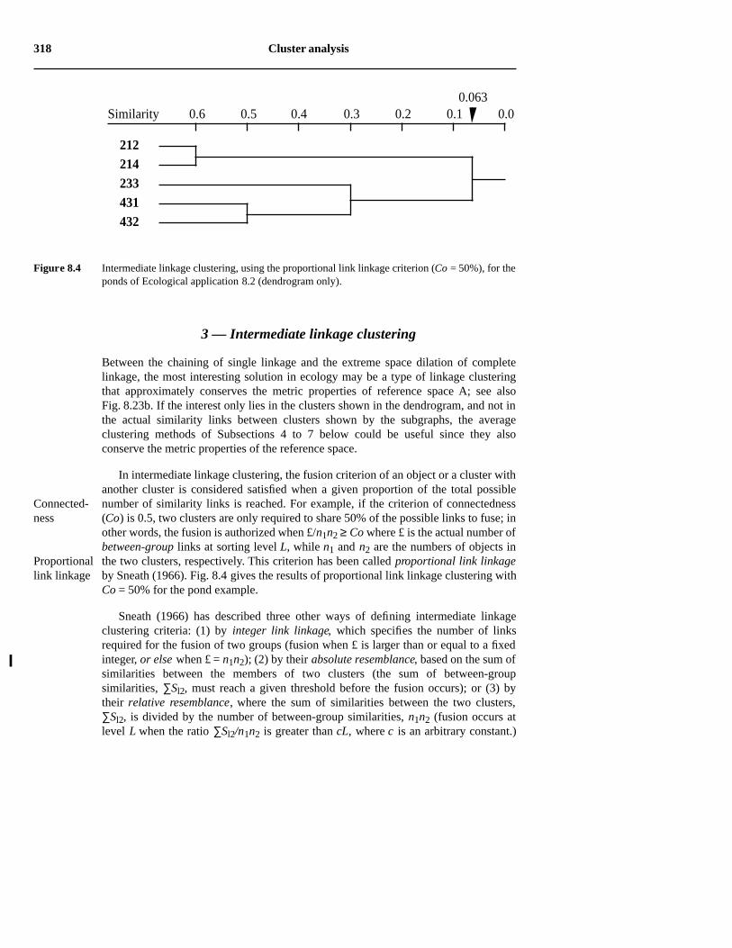
In intermediate linkage clustering, the fusion criterion of an object or a cluster withanother cluster is considered satisfied when a given proportion of the total possiblenumber of similarity links is reached. For example, if the criterion of connectedness(Co) is 0.5, two clusters are only required to share 50% of the possible links to fuse; inother words, the fusion is authorized when £/n1n2 ≥ Co where £ is the actual number ofbetween-group links at sorting level L, while n1 and n2 are the numbers of objects inthe two clusters, respectively. This criterion has been called proportional link linkageby Sneath (1966). Fig. 8.4 gives the results of proportional link linkage clustering withCo = 50% for the pond example.
Sneath (1966) has described three other ways of defining intermediate linkageclustering criteria: (1) by integer link linkage, which specifies the number of linksrequired for the fusion of two groups (fusion when £ is larger than or equal to a fixedinteger, or else when £ = n1n2); (2) by their absolute resemblance, based on the sum ofsimilarities between the members of two clusters (the sum of between-groupsimilarities, ∑Sl2, must reach a given threshold before the fusion occurs); or (3) bytheir relative resemblance, where the sum of similarities between the two clusters,∑Sl2, is divided by the number of between-group similarities, n1n2 (fusion occurs atlevel L when the ratio ∑Sl2/n1n2 is greater than cL, where c is an arbitrary constant.)
Connected-ness
Proportionallink linkage
Figure 8.4 Intermediate linkage clustering, using the proportional link linkage criterion (Co = 50%), for theponds of Ecological application 8.2 (dendrogram only).
Similarity 0.6 0.5 0.4 0.3 0.2 0.1 0.0
212214233431432
0.063
Hierarchical agglomerative clustering 319
When c equals 1, the method is called average linkage clustering. These strategies arenot combinatorial in the sense of Subsection 8.5.9.
4 — Unweighted arithmetic average clustering (UPGMA)
There are four methods of average clustering that conserve the metric properties ofreference space A. These four methods were called “average linkage clustering” bySneath & Sokal (1973), although they do not tally the links between clusters. As aconsequence they are not object-linkage methods in the sense of the previous threesubsections. They rely instead on average similarities among objects or on centroids ofclusters. The four methods have nothing to do with Sneath’s (1966) “average linkageclustering” described in the previous paragraph, so that we prefer calling them“average clustering”. These methods (Table 8.2) result from the combinations of twodichotomies: (1) arithmetic average versus centroid clustering and (2) weightingversus non-weighting.
The first method in Table 8.2 is the unweighted arithmetic average clustering(Rohlf, 1963), also called “UPGMA” (“Unweighted Pair-Group Method usingArithmetic averages”) by Sneath & Sokal (1973) or “group-average sorting” by Lance& Williams (1966a and 1967c). It is also called “average linkage” by SAS, SYSTAT
and some other statistical packages, thus adding to the confusion pointed out in theprevious paragraph. The highest similarity (or smallest distance) identifies the nextcluster to be formed. Following this event, the method computes the arithmeticaverage of the similarities or distances between a candidate object and each of thecluster members or, in the case of a previously formed cluster, between all members ofthe two clusters. All objects receive equal weights in the computation. The similarityor distance matrix is updated and reduced in size at each clustering step. Clusteringproceeds by agglomeration as the similarity criterion is relaxed, just as it does in singlelinkage clustering.
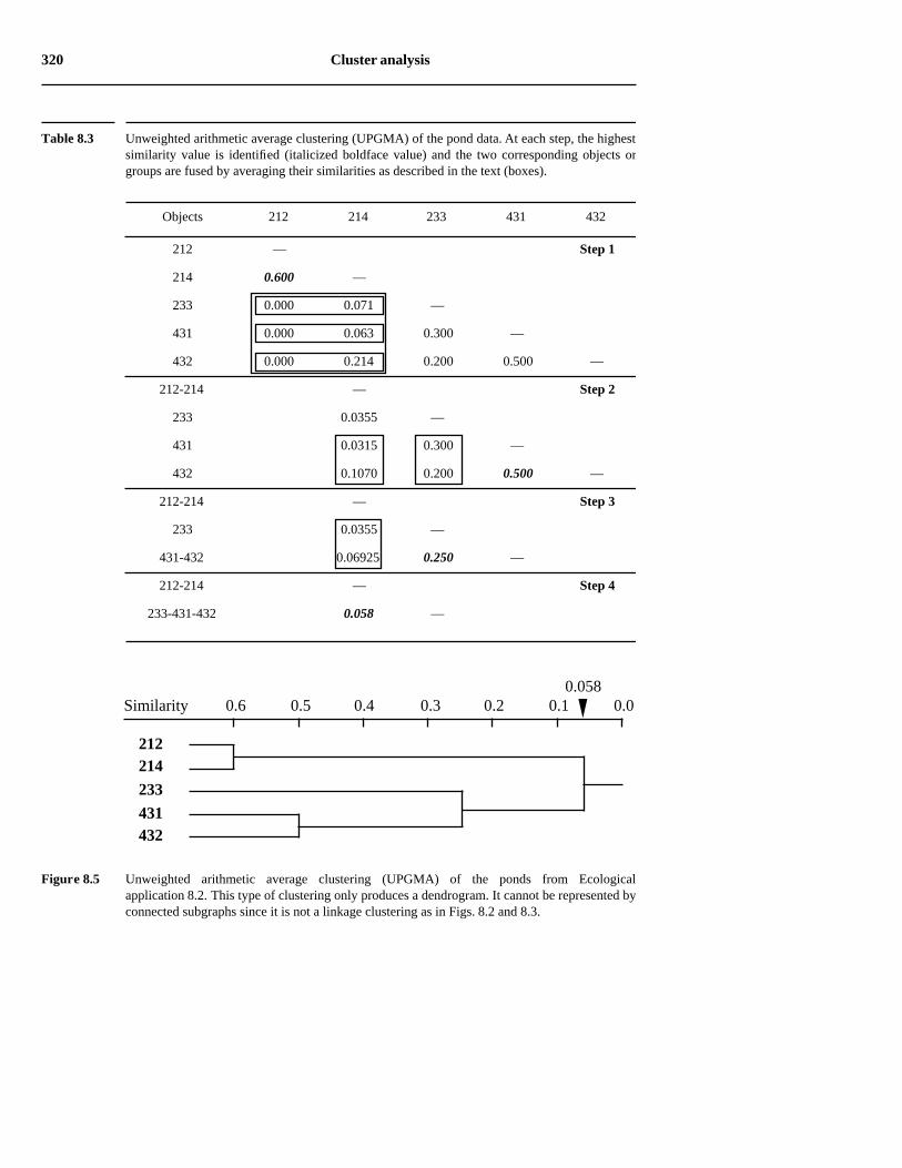
For the ponds of Section 8.2, UPGMA clustering proceeds as shown in Table 8.3and Fig. 8.5. At step 1, the highest similarity value in the matrix is
Averageclustering
Table 8.2 Average clustering methods discussed in Subsections 8.5.4 to 8.5.7.
Arithmetic average Centroid clustering
Equal weights 4. Unweighted arithmetic 6. Unweighted centroidaverage clustering (UPGMA) clustering (UPGMC)
Unequal weights 5. Weighted arithmetic 7. Weighted centroid average clustering (WPGMA) clustering (WPGMC)
320 Cluster analysis
Table 8.3 Unweighted arithmetic average clustering (UPGMA) of the pond data. At each step, the highestsimilarity value is identified (italicized boldface value) and the two corresponding objects orgroups are fused by averaging their similarities as described in the text (boxes).
Objects 212 214 233 431 432
Figure 8.5 Unweighted arithmetic average clustering (UPGMA) of the ponds from Ecologicalapplication 8.2. This type of clustering only produces a dendrogram. It cannot be represented byconnected subgraphs since it is not a linkage clustering as in Figs. 8.2 and 8.3.
212 — Step 1
214 0.600 —
233 0.000 0.071 —
431 0.000 0.063 0.300 —
432 0.000 0.214 0.200 0.500 —
212-214 — Step 2
233 0.0355 —
431 0.0315 0.300 —
432 0.1070 0.200 0.500 —
212-214 — Step 3
233 0.0355 —
431-432 0.06925 0.250 —
212-214 — Step 4
233-431-432 0.058 —
Similarity 0.6 0.5 0.4 0.3 0.2 0.1 0.0
212214
233
431432
0.058
Hierarchical agglomerative clustering 321
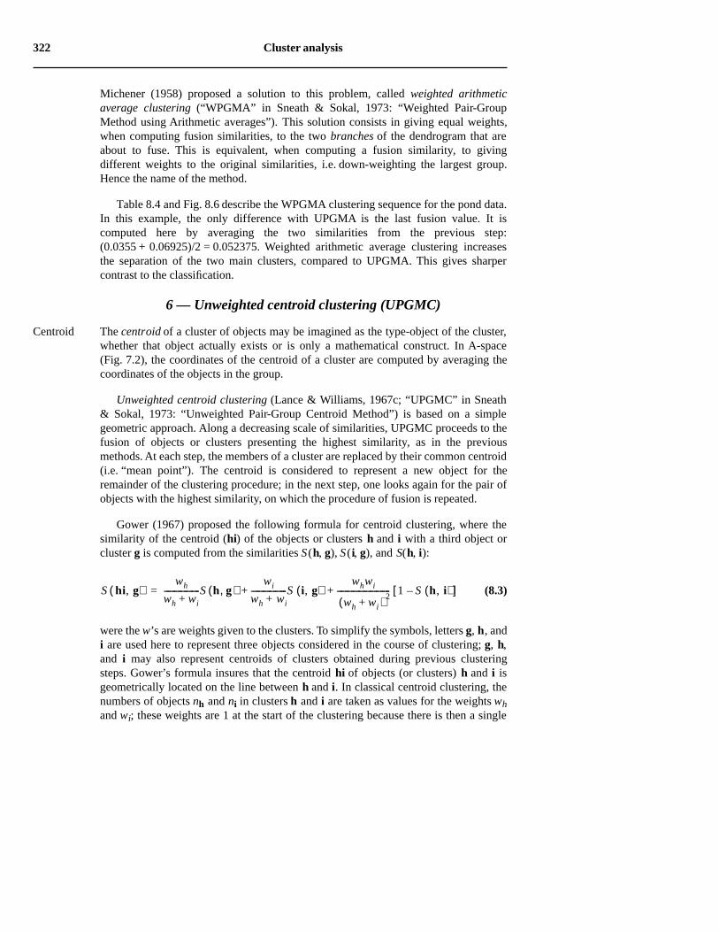
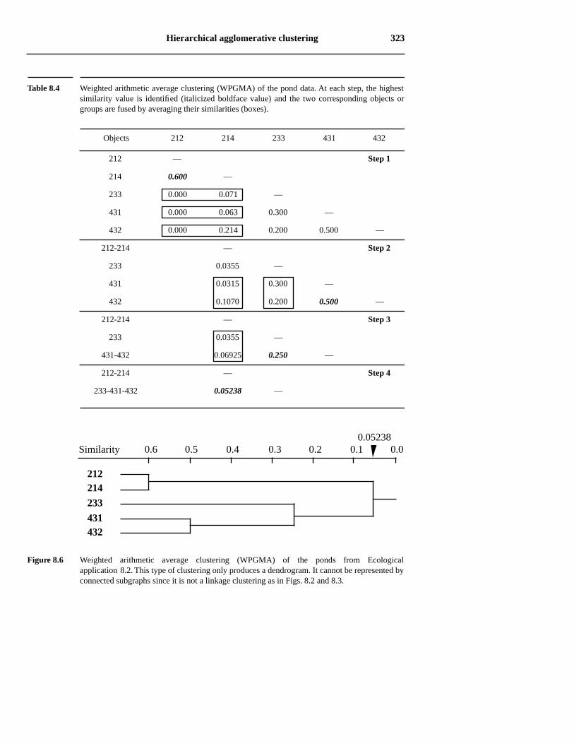
S (212, 214) = 0.600; hence the two objects fuse at level 0.600. As a consequence ofthis fusion, the similarity values of these two objects with each of the remainingobjects in the study must be averaged (values in the inner boxes in the Table, step 1);this results in a reduction of the size of the similarity matrix. Considering the reducedmatrix (step 2), the highest similarity value is S = 0.500; it indicates that objects 431and 432 fuse at level 0.500. Again, this similarity value is obtained by averaging theboxed values; this produces a new reduced similarity matrix for the next step. In step3, the largest similarity is 0.250; it leads to the fusion of the already-formed group(431, 432) with object 233 at level 0.250. In the example, this last fusion is the difficultpoint to understand. Before averaging the values, each one is multiplied by the numberof objects in the corresponding group. There is one object in group (233) and two ingroup (431, 432), so that the fused similarity value is calculated as [(0.0355 × 1) +(0.06925 × 2)]/3 = 0.058. This is equivalent to averaging the six boxed similarities inthe top matrix (larger box) with equal weights; the result would also be 0.058. So, thismethod is “unweighted” in the sense that it gives equal weights to the originalsimilarities. To achieve this at step 3, one has to use weights that are equal to thenumber of objects in the groups. At step 4, there is a single remaining similarity value;it is used to perform the last fusion at level 0.058. In the dendrogram, fusions aredrawn at the identified levels.
Because it gives equal weights to the original similarities, the UPGMA methodassumes that the objects in each group form a representative sample of thecorresponding larger groups of objects in the reference population under study. Forthat reason, UPGMA clustering should only be used in connection with simple randomor systematic sampling designs if the results are to be extrapolated to some largerreference population.
Unlike linkage clustering methods, information about the relationships betweenpairs of objects is lost in methods based on progressive reduction of the similaritymatrix, since only the relationships among groups are considered. This informationmay be extracted from the original similarity matrix, by making a list of the strongestsimilarity link found, at each fusion level, between the objects of the two groups. Forthe pond example, the chain of primary connections corresponding to the dendrogramwould be made of the following links: (212, 214) for the first fusion level, (431, 432)for the second level, (233, 431) for the third level, and (214, 432) for the last level(Table 8.3, step 1). The topology obtained from UPGMA clustering may differ fromthat of single linkage; if this had been the case here, the chain of primary connectionswould have been different from that of single linkage clustering.
5 — Weighted arithmetic average clustering (WPGMA)
It often occurs in ecology that groups of objects, representing different regions of aterritory, are of unequal sizes. Eliminating objects to equalize the clusters would meandiscarding valuable information. However, the presence of a large group of objects,which are more similar a priori because of their common origin, may distort theUPGMA results when a fusion occurs with a smaller group of objects. Sokal &
322 Cluster analysis
Michener (1958) proposed a solution to this problem, called weighted arithmeticaverage clustering (“WPGMA” in Sneath & Sokal, 1973: “Weighted Pair-GroupMethod using Arithmetic averages”). This solution consists in giving equal weights,when computing fusion similarities, to the two branches of the dendrogram that areabout to fuse. This is equivalent, when computing a fusion similarity, to givingdifferent weights to the original similarities, i.e. down-weighting the largest group.Hence the name of the method.
Table 8.4 and Fig. 8.6 describe the WPGMA clustering sequence for the pond data.In this example, the only difference with UPGMA is the last fusion value. It iscomputed here by averaging the two similarities from the previous step:(0.0355 + 0.06925)/2 = 0.052375. Weighted arithmetic average clustering increasesthe separation of the two main clusters, compared to UPGMA. This gives sharpercontrast to the classification.
6 — Unweighted centroid clustering (UPGMC)
The centroid of a cluster of objects may be imagined as the type-object of the cluster,whether that object actually exists or is only a mathematical construct. In A-space(Fig. 7.2), the coordinates of the centroid of a cluster are computed by averaging thecoordinates of the objects in the group.
Unweighted centroid clustering (Lance & Williams, 1967c; “UPGMC” in Sneath& Sokal, 1973: “Unweighted Pair-Group Centroid Method”) is based on a simplegeometric approach. Along a decreasing scale of similarities, UPGMC proceeds to thefusion of objects or clusters presenting the highest similarity, as in the previousmethods. At each step, the members of a cluster are replaced by their common centroid(i.e. “mean point”). The centroid is considered to represent a new object for theremainder of the clustering procedure; in the next step, one looks again for the pair ofobjects with the highest similarity, on which the procedure of fusion is repeated.
Gower (1967) proposed the following formula for centroid clustering, where thesimilarity of the centroid (hi) of the objects or clusters h and i with a third object orcluster g is computed from the similarities S (h, g), S (i, g), and S(h, i):
(8.3)
were the w’s are weights given to the clusters. To simplify the symbols, letters g, h, andi are used here to represent three objects considered in the course of clustering; g, h,and i may also represent centroids of clusters obtained during previous clusteringsteps. Gower’s formula insures that the centroid hi of objects (or clusters) h and i isgeometrically located on the line between h and i. In classical centroid clustering, thenumbers of objects nh and ni in clusters h and i are taken as values for the weights whand wi; these weights are 1 at the start of the clustering because there is then a single
Centroid
S hi, g( )wh
wh wi+------------------S h g,( )
wi
wh wi+------------------S i, g( )
whwi
wh wi+( ) 2--------------------------- 1 S h, i( )–[ ]+ +=
Hierarchical agglomerative clustering 323
Table 8.4 Weighted arithmetic average clustering (WPGMA) of the pond data. At each step, the highestsimilarity value is identified (italicized boldface value) and the two corresponding objects orgroups are fused by averaging their similarities (boxes).
Objects 212 214 233 431 432
Figure 8.6 Weighted arithmetic average clustering (WPGMA) of the ponds from Ecologicalapplication 8.2. This type of clustering only produces a dendrogram. It cannot be represented byconnected subgraphs since it is not a linkage clustering as in Figs. 8.2 and 8.3.
212 — Step 1
214 0.600 —
233 0.000 0.071 —
431 0.000 0.063 0.300 —
432 0.000 0.214 0.200 0.500 —
212-214 — Step 2
233 0.0355 —
431 0.0315 0.300 —
432 0.1070 0.200 0.500 —
212-214 — Step 3
233 0.0355 —
431-432 0.06925 0.250 —
212-214 — Step 4
233-431-432 0.05238 —
Similarity 0.6 0.5 0.4 0.3 0.2 0.1 0.0
212214
233
431432
0.05238
324 Cluster analysis
object per cluster. If initial weights are attached to individual objects, they may be usedinstead of 1’s in eq. 8.3.
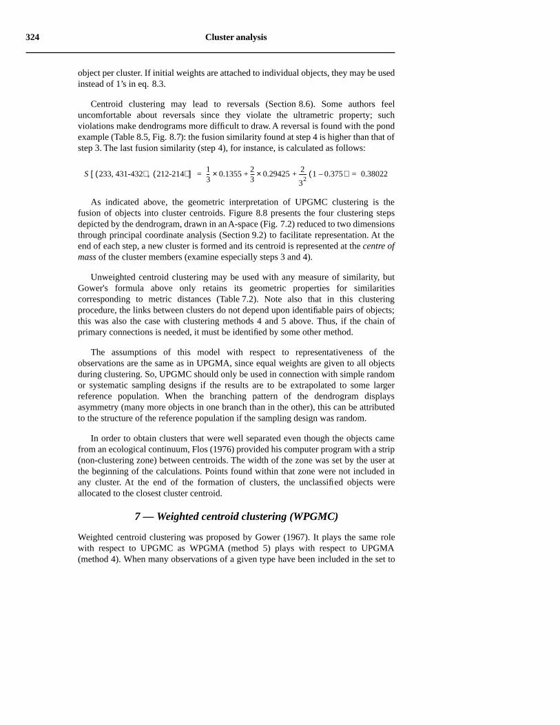
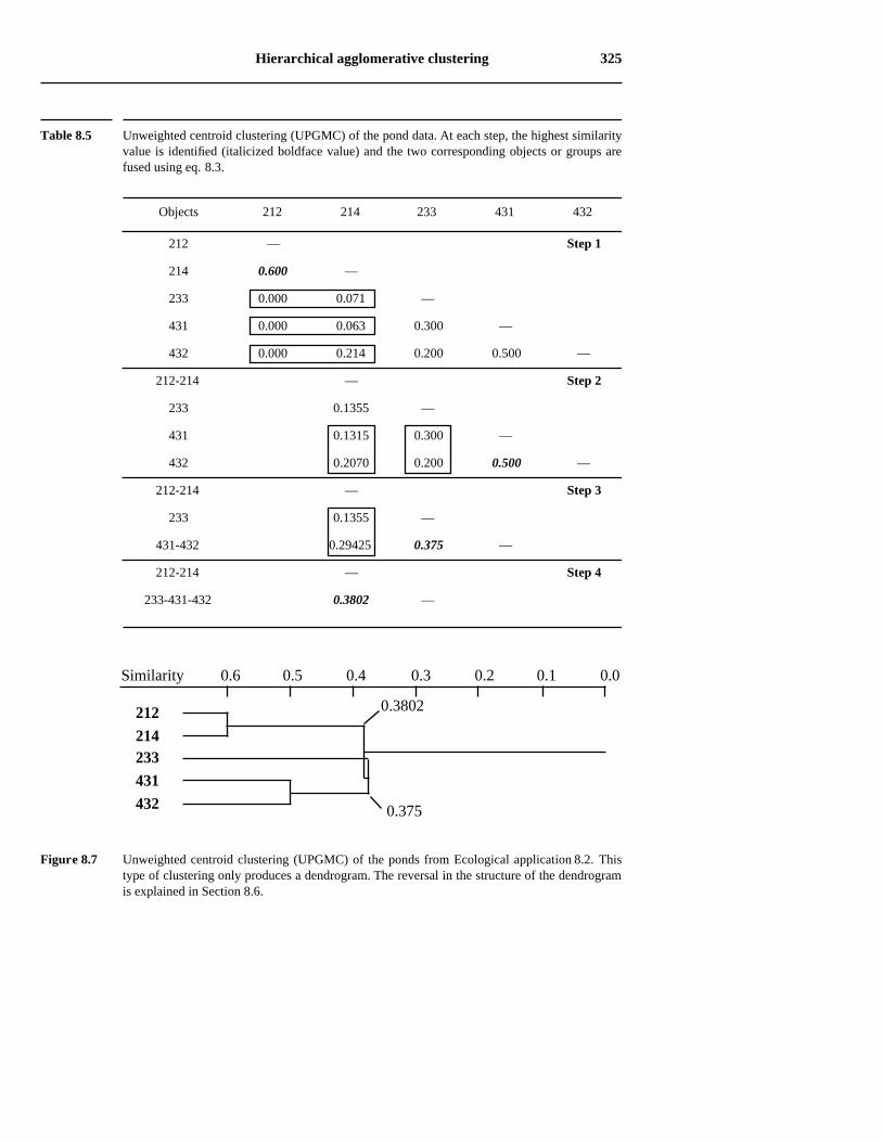
Centroid clustering may lead to reversals (Section 8.6). Some authors feeluncomfortable about reversals since they violate the ultrametric property; suchviolations make dendrograms more difficult to draw. A reversal is found with the pondexample (Table 8.5, Fig. 8.7): the fusion similarity found at step 4 is higher than that ofstep 3. The last fusion similarity (step 4), for instance, is calculated as follows:
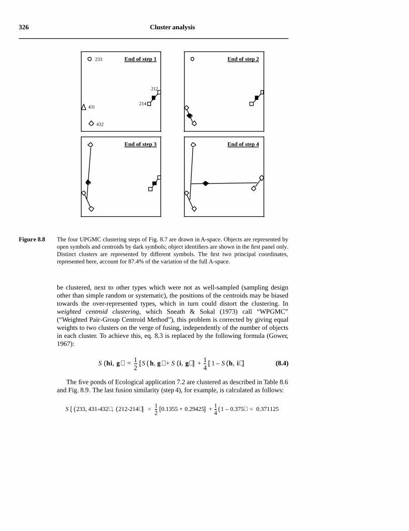
As indicated above, the geometric interpretation of UPGMC clustering is thefusion of objects into cluster centroids. Figure 8.8 presents the four clustering stepsdepicted by the dendrogram, drawn in an A-space (Fig. 7.2) reduced to two dimensionsthrough principal coordinate analysis (Section 9.2) to facilitate representation. At theend of each step, a new cluster is formed and its centroid is represented at the centre ofmass of the cluster members (examine especially steps 3 and 4).
Unweighted centroid clustering may be used with any measure of similarity, butGower's formula above only retains its geometric properties for similaritiescorresponding to metric distances (Table 7.2). Note also that in this clusteringprocedure, the links between clusters do not depend upon identifiable pairs of objects;this was also the case with clustering methods 4 and 5 above. Thus, if the chain ofprimary connections is needed, it must be identified by some other method.
The assumptions of this model with respect to representativeness of theobservations are the same as in UPGMA, since equal weights are given to all objectsduring clustering. So, UPGMC should only be used in connection with simple randomor systematic sampling designs if the results are to be extrapolated to some largerreference population. When the branching pattern of the dendrogram displaysasymmetry (many more objects in one branch than in the other), this can be attributedto the structure of the reference population if the sampling design was random.
In order to obtain clusters that were well separated even though the objects camefrom an ecological continuum, Flos (1976) provided his computer program with a strip(non-clustering zone) between centroids. The width of the zone was set by the user atthe beginning of the calculations. Points found within that zone were not included inany cluster. At the end of the formation of clusters, the unclassified objects wereallocated to the closest cluster centroid.
7 — Weighted centroid clustering (WPGMC)
Weighted centroid clustering was proposed by Gower (1967). It plays the same rolewith respect to UPGMC as WPGMA (method 5) plays with respect to UPGMA(method 4). When many observations of a given type have been included in the set to
S 233, 431-432( ) 212-214( ),[ ] 13--- 0.1355× 2
3--- 0.29425× 2
32----- 1 0.375–( )+ + 0.38022= =
Hierarchical agglomerative clustering 325
Table 8.5 Unweighted centroid clustering (UPGMC) of the pond data. At each step, the highest similarityvalue is identified (italicized boldface value) and the two corresponding objects or groups arefused using eq. 8.3.
Objects 212 214 233 431 432
Figure 8.7 Unweighted centroid clustering (UPGMC) of the ponds from Ecological application 8.2. Thistype of clustering only produces a dendrogram. The reversal in the structure of the dendrogramis explained in Section 8.6.
212 — Step 1
214 0.600 —
233 0.000 0.071 —
431 0.000 0.063 0.300 —
432 0.000 0.214 0.200 0.500 —
212-214 — Step 2
233 0.1355 —
431 0.1315 0.300 —
432 0.2070 0.200 0.500 —
212-214 — Step 3
233 0.1355 —
431-432 0.29425 0.375 —
212-214 — Step 4
233-431-432 0.3802 —
Similarity 0.6 0.5 0.4 0.3 0.2 0.1 0.0
212
214233
431
432
0.3802
0.375
326 Cluster analysis
be clustered, next to other types which were not as well-sampled (sampling designother than simple random or systematic), the positions of the centroids may be biasedtowards the over-represented types, which in turn could distort the clustering. Inweighted centroid clustering, which Sneath & Sokal (1973) call “WPGMC”(“Weighted Pair-Group Centroid Method”), this problem is corrected by giving equalweights to two clusters on the verge of fusing, independently of the number of objectsin each cluster. To achieve this, eq. 8.3 is replaced by the following formula (Gower,1967):
(8.4)
The five ponds of Ecological application 7.2 are clustered as described in Table 8.6and Fig. 8.9. The last fusion similarity (step 4), for example, is calculated as follows:
Figure 8.8 The four UPGMC clustering steps of Fig. 8.7 are drawn in A-space. Objects are represented byopen symbols and centroids by dark symbols; object identifiers are shown in the first panel only.Distinct clusters are represented by different symbols. The first two principal coordinates,represented here, account for 87.4% of the variation of the full A-space.
212
214
233
431
432
End of step 1
End of step 4
End of step 2
End of step 3
S hi, g( ) 12--- S h, g( ) S i, g( )+[ ] 1
4--- 1 S h, i( )–[ ]+=
S 233, 431-432( ) 212-214( ),[ ] 12--- 0.1355 0.29425+[ ] 1
4--- 1 0.375–( )+ 0.371125= =
Hierarchical agglomerative clustering 327
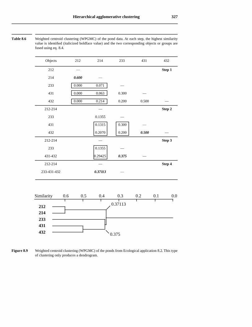
Table 8.6 Weighted centroid clustering (WPGMC) of the pond data. At each step, the highest similarityvalue is identified (italicized boldface value) and the two corresponding objects or groups arefused using eq. 8.4.
Objects 212 214 233 431 432
Figure 8.9 Weighted centroid clustering (WPGMC) of the ponds from Ecological application 8.2. This typeof clustering only produces a dendrogram.
212 — Step 1
214 0.600 —
233 0.000 0.071 —
431 0.000 0.063 0.300 —
432 0.000 0.214 0.200 0.500 —
212-214 — Step 2
233 0.1355 —
431 0.1315 0.300 —
432 0.2070 0.200 0.500 —
212-214 — Step 3
233 0.1355 —
431-432 0.29425 0.375 —
212-214 — Step 4
233-431-432 0.37113 —
Similarity 0.6 0.5 0.4 0.3 0.2 0.1 0.0
212214
233431
432
0.37113
0.375
328 Cluster analysis
This value is the level at which the next fusion takes place. Note that no reversalappears in this result, although WPGMC may occasionally produce reversals, likeUPGMC clustering.
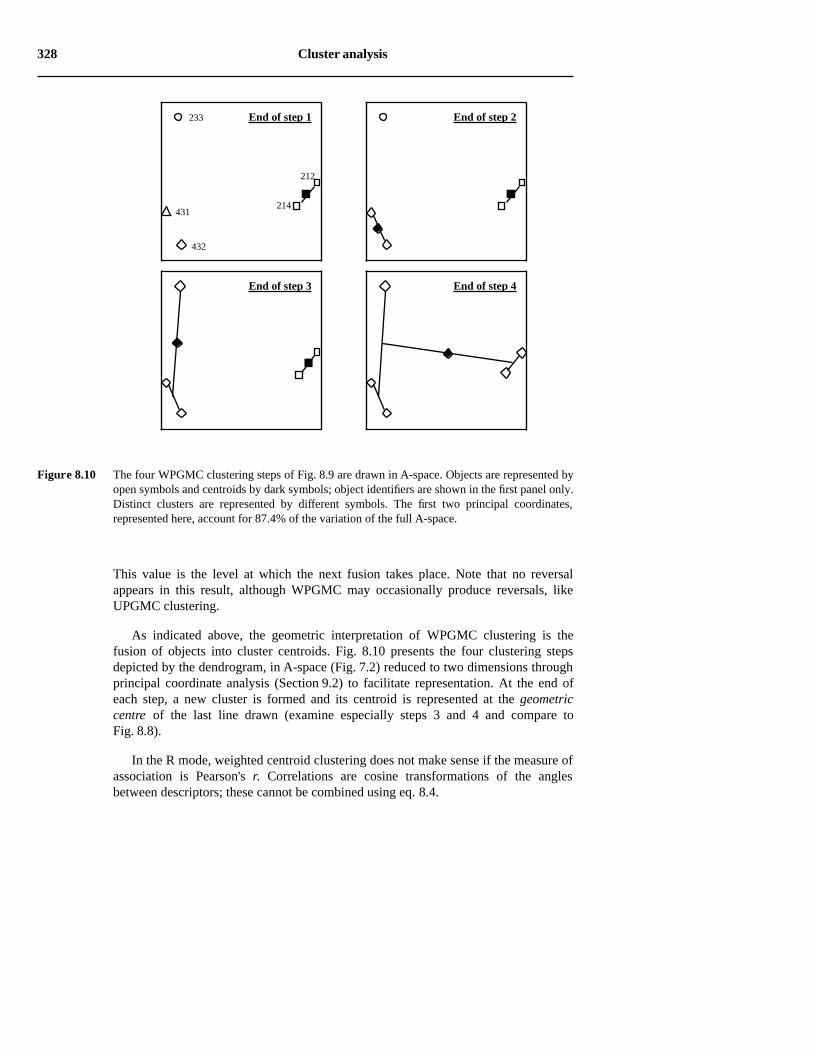
As indicated above, the geometric interpretation of WPGMC clustering is thefusion of objects into cluster centroids. Fig. 8.10 presents the four clustering stepsdepicted by the dendrogram, in A-space (Fig. 7.2) reduced to two dimensions throughprincipal coordinate analysis (Section 9.2) to facilitate representation. At the end ofeach step, a new cluster is formed and its centroid is represented at the geometriccentre of the last line drawn (examine especially steps 3 and 4 and compare toFig. 8.8).
In the R mode, weighted centroid clustering does not make sense if the measure ofassociation is Pearson's r. Correlations are cosine transformations of the anglesbetween descriptors; these cannot be combined using eq. 8.4.
Figure 8.10 The four WPGMC clustering steps of Fig. 8.9 are drawn in A-space. Objects are represented byopen symbols and centroids by dark symbols; object identifiers are shown in the first panel only.Distinct clusters are represented by different symbols. The first two principal coordinates,represented here, account for 87.4% of the variation of the full A-space.
212
214
233
431
432
End of step 4End of step 3
End of step 2End of step 1
Hierarchical agglomerative clustering 329
8 — Ward’s minimum variance method
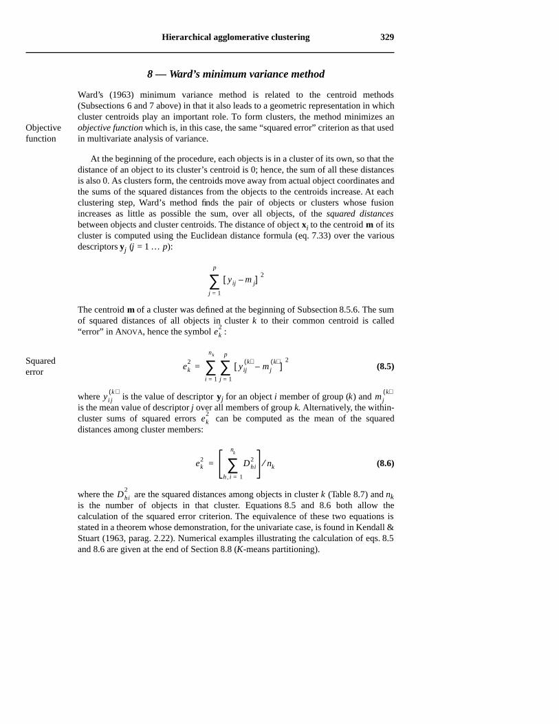
Ward’s (1963) minimum variance method is related to the centroid methods(Subsections 6 and 7 above) in that it also leads to a geometric representation in whichcluster centroids play an important role. To form clusters, the method minimizes anobjective function which is, in this case, the same “squared error” criterion as that usedin multivariate analysis of variance.
At the beginning of the procedure, each objects is in a cluster of its own, so that thedistance of an object to its cluster’s centroid is 0; hence, the sum of all these distancesis also 0. As clusters form, the centroids move away from actual object coordinates andthe sums of the squared distances from the objects to the centroids increase. At eachclustering step, Ward’s method finds the pair of objects or clusters whose fusionincreases as little as possible the sum, over all objects, of the squared distancesbetween objects and cluster centroids. The distance of object xi to the centroid m of itscluster is computed using the Euclidean distance formula (eq. 7.33) over the variousdescriptors yj (j = 1 … p):
The centroid m of a cluster was defined at the beginning of Subsection 8.5.6. The sumof squared distances of all objects in cluster k to their common centroid is called“error” in ANOVA, hence the symbol :
(8.5)
where is the value of descriptor yj for an object i member of group (k) and is the mean value of descriptor j over all members of group k. Alternatively, the within-cluster sums of squared errors can be computed as the mean of the squareddistances among cluster members:
(8.6)
where the are the squared distances among objects in cluster k (Table 8.7) and nkis the number of objects in that cluster. Equations 8.5 and 8.6 both allow thecalculation of the squared error criterion. The equivalence of these two equations isstated in a theorem whose demonstration, for the univariate case, is found in Kendall &Stuart (1963, parag. 2.22). Numerical examples illustrating the calculation of eqs. 8.5and 8.6 are given at the end of Section 8.8 (K-means partitioning).
Objectivefunction
yij m j–[ ] 2
j 1=
p
∑
ek2
Squarederror
ek2
yijk( )
m jk( )
–[ ]2
j 1=
p
∑i 1=
nk
∑=
yi jk( )
m jk( )
ek2
ek2 Dhi
2
h i, 1=
nk
∑ nk⁄=
Dhi2
330 Cluster analysis
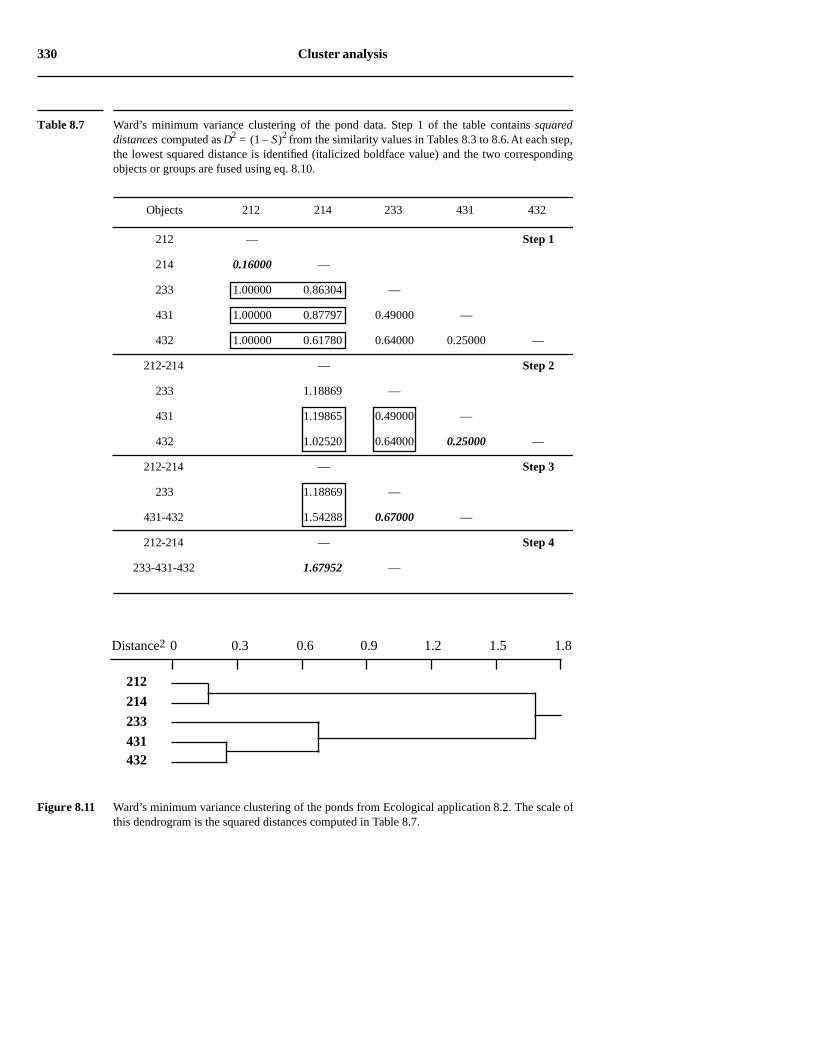
Table 8.7 Ward’s minimum variance clustering of the pond data. Step 1 of the table contains squareddistances computed as D2 = (1 – S)2 from the similarity values in Tables 8.3 to 8.6. At each step,the lowest squared distance is identified (italicized boldface value) and the two correspondingobjects or groups are fused using eq. 8.10.
Objects 212 214 233 431 432
Figure 8.11 Ward’s minimum variance clustering of the ponds from Ecological application 8.2. The scale ofthis dendrogram is the squared distances computed in Table 8.7.
212 — Step 1
214 0.16000 —
233 1.00000 0.86304 —
431 1.00000 0.87797 0.49000 —
432 1.00000 0.61780 0.64000 0.25000 —
212-214 — Step 2
233 1.18869 —
431 1.19865 0.49000 —
432 1.02520 0.64000 0.25000 —
212-214 — Step 3
233 1.18869 —
431-432 1.54288 0.67000 —
212-214 — Step 4
233-431-432 1.67952 —
Distance2
212214233431432
1.81.2 1.50.90.60.30
Hierarchical agglomerative clustering 331
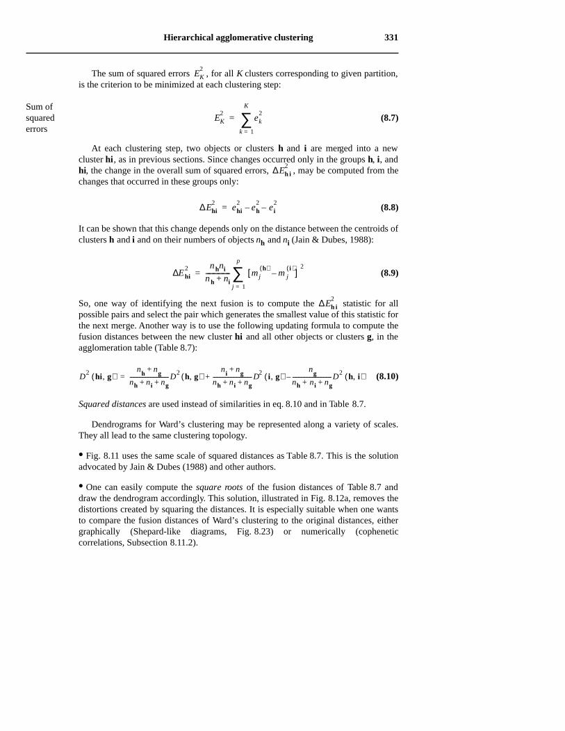
The sum of squared errors , for all K clusters corresponding to given partition,is the criterion to be minimized at each clustering step:
(8.7)
At each clustering step, two objects or clusters h and i are merged into a newcluster hi, as in previous sections. Since changes occurred only in the groups h, i, andhi, the change in the overall sum of squared errors, , may be computed from thechanges that occurred in these groups only:
(8.8)
It can be shown that this change depends only on the distance between the centroids ofclusters h and i and on their numbers of objects nh and ni (Jain & Dubes, 1988):
(8.9)
So, one way of identifying the next fusion is to compute the statistic for allpossible pairs and select the pair which generates the smallest value of this statistic forthe next merge. Another way is to use the following updating formula to compute thefusion distances between the new cluster hi and all other objects or clusters g, in theagglomeration table (Table 8.7):
(8.10)
Squared distances are used instead of similarities in eq. 8.10 and in Table 8.7.
Dendrograms for Ward’s clustering may be represented along a variety of scales.They all lead to the same clustering topology.
• Fig. 8.11 uses the same scale of squared distances as Table 8.7. This is the solutionadvocated by Jain & Dubes (1988) and other authors.
• One can easily compute the square roots of the fusion distances of Table 8.7 anddraw the dendrogram accordingly. This solution, illustrated in Fig. 8.12a, removes thedistortions created by squaring the distances. It is especially suitable when one wantsto compare the fusion distances of Ward’s clustering to the original distances, eithergraphically (Shepard-like diagrams, Fig. 8.23) or numerically (copheneticcorrelations, Subsection 8.11.2).
EK2
Sum ofsquarederrors
EK2
ek2
k 1=
K
∑=
∆Eh i2
∆Ehi2
ehi2
eh2
ei2
––=
∆Ehi2 nhni
nh ni+---------------- m j
h( )m j
i( )–[ ]
2
j 1=
p
∑=
∆Eh i2
D2 hi, g( )
nh ng+
nh ni ng+ +----------------------------D
2 h, g( )ni ng+
nh ni ng+ +----------------------------D
2 i, g( )ng
nh ni ng+ +----------------------------D
2 h, i( )–+=
332 Cluster analysis
• The sum of squared errors (eq. 8.7) is used in some computer programs as theclustering scale. This statistic is also called the total error sum of squares (TESS) byEveritt (1980) and other authors. This solution is illustrated in Fig. 8.12b.
• The SAS package (1985) recommends two scales for Ward’s clustering. The first oneis the proportion of variance (R2) accounted for by the clusters at any given partitionlevel. It is computed as the total sum of squares (i.e. the sum of squared distances fromthe centroid of all objects) minus the within-cluster squared errors of eq. 8.7 forthe given partition, divided by the total sum of squares. R2 decreases as clusters grow.When all the objects are lumped in a single cluster, the resulting one-cluster partitiondoes not explain any of the objects’ variation so that R2 = 0. The second scalerecommended by SAS is called the semipartial R2. It is computed as the between-cluster sum of squares divided by the (corrected) total sum of squares. This statisticincreases as the clusters grow.
Like the K-means partitioning method (Section 8.8), Ward’s agglomerativeclustering can be computed from either a raw data table using eq. 8.8, or a matrix ofsquared distances through eq. 8.10. The latter is the most usual approach in computerprograms. It is important to note that distances are computed as (squared) Euclidean
EK2
TESS
Figure 8.12 Ward’s minimum variance clustering of the ponds from Ecological application 8.2. The scale ofdendrogram (a) is the square root of the squared distances computed in Table 8.7; in dendrogram(b), it is the (or TESS) statistic.EK
2
Distance
212
214233
431432
1.81.2 1.50.90.60.30
(a)
EK
212
214233
431432
1.81.2 1.50.90.60.302
(b)
EK2
Hierarchical agglomerative clustering 333
distances in Ward’s method. So, unless the descriptors are such that Euclideandistances (D1 in Chapter 7) are an appropriate model for the relationships amongobjects, one should not use a Ward’s algorithm based or raw data. It is preferable insuch cases to compute a distance matrix using an appropriate coefficient (Tables 7.3 to7.5), followed by clustering of the resemblance matrix in A-space by a distance-basedWard algorithm. Section 9.2 will show that resemblance matrices can also be used forplotting the positions of objects in A-space, “as if” the distances were Euclidean.
Because of the squared error criterion used as the objective function to minimize,clusters produced by the Ward minimum variance method tend to be hyperspherical,i.e. spherical in multidimensional A-space, and to contain roughly the same number ofobjects if the observations are evenly distributed through A-space. The same applies tothe centroid methods of the previous subsections. This may be seen as either anadvantage or a problem, depending on the researcher’s conceptual model of a cluster.
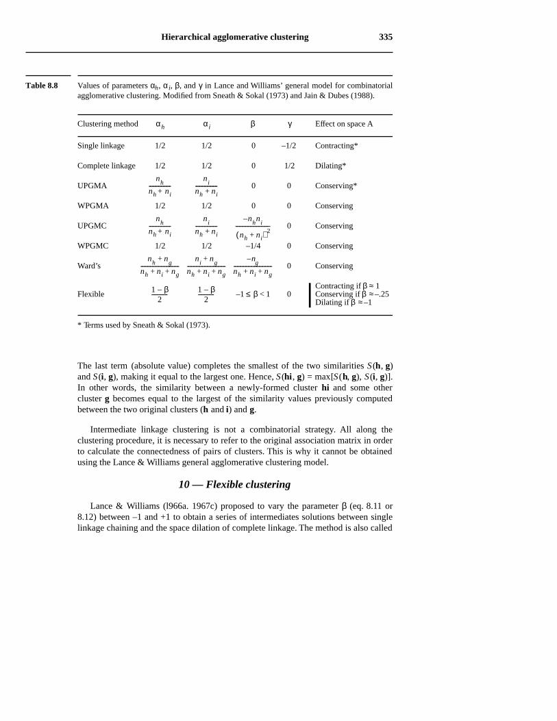
9 — General agglomerative clustering model
Lance & Williams (1966a, 1967c) have proposed a general model that encompasses allthe agglomerative clustering methods presented up to now, except intermediatelinkage (Subsection 3). The general model offers the advantage of being translatableinto a single, simple computer program, so that it is used in most statistical packagesthat offer agglomerative clustering. The general model allows one to select anagglomerative clustering model by choosing the values of four parameters, called αh,αi , β, and γ, which determine the clustering strategy. This model only outputs thebranching pattern of the clustering tree (the dendrogram), as it was the case for themethods described in Subsections 8.5.4 to 8.5.8. For the linkage clustering strategies(Subsections 8.5.1 to 8.5.3), the list of links responsible for cluster formation may beobtained afterwards by comparing the dendrogram to the similarity matrix.
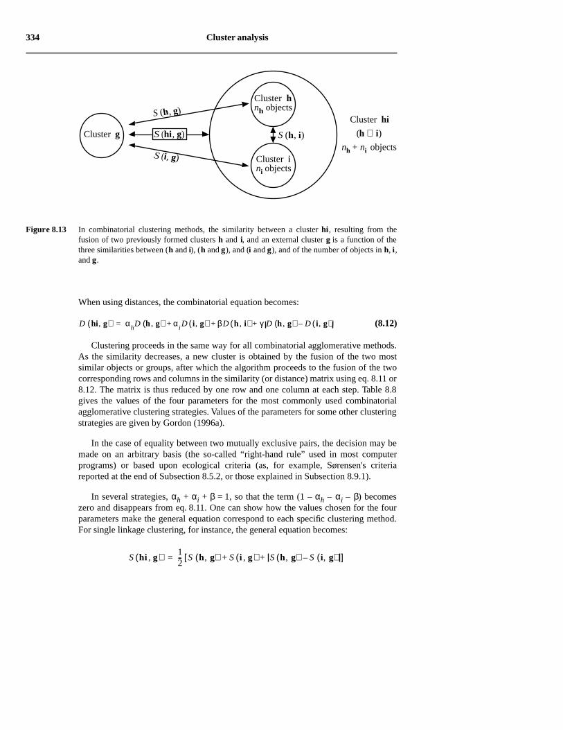
The model of Lance & Williams is limited to combinatorial clustering methods,i.e. those for which the similarity S (hi, g) between an external cluster g and a clusterhi, resulting from the prior fusion of clusters h and i, is a function of the threesimilarities S (h, g), S (i, g), and S (h, i) and also, eventually, the numbers nh, ni , and ngof objects in clusters h, i, and g, respectively (Fig. 8.13). Individual objects areconsidered to be single-member clusters. Since the similarity of cluster hi with anexternal cluster g can be computed from the above six values, h and i can becondensed into a single row and a single column in the updated similarity matrix;following that, the clustering proceeds as in the Tables of the previous Subsections.Since the new similarities at each step can be computed by combining those from theprevious step, it is not necessary for a computer program to retain the originalsimilarity matrix or data set. Non-combinatorial methods do not have this property. Forsimilarities, the general model for combinatorial methods is the following:
(8.11)
Combina-torial method
S hi, g( ) 1 αh
αi
–– β–( ) αh
+ S h, g( ) αiS i, g( )+ βS h , i( ) γ S h , g( ) S i, g( )––+=
334 Cluster analysis
When using distances, the combinatorial equation becomes:
(8.12)
Clustering proceeds in the same way for all combinatorial agglomerative methods.As the similarity decreases, a new cluster is obtained by the fusion of the two mostsimilar objects or groups, after which the algorithm proceeds to the fusion of the twocorresponding rows and columns in the similarity (or distance) matrix using eq. 8.11 or8.12. The matrix is thus reduced by one row and one column at each step. Table 8.8gives the values of the four parameters for the most commonly used combinatorialagglomerative clustering strategies. Values of the parameters for some other clusteringstrategies are given by Gordon (1996a).
In the case of equality between two mutually exclusive pairs, the decision may bemade on an arbitrary basis (the so-called “right-hand rule” used in most computerprograms) or based upon ecological criteria (as, for example, Sørensen's criteriareported at the end of Subsection 8.5.2, or those explained in Subsection 8.9.1).
In several strategies, αh + αi + β = 1, so that the term (1 – αh – αi – β) becomeszero and disappears from eq. 8.11. One can show how the values chosen for the fourparameters make the general equation correspond to each specific clustering method.For single linkage clustering, for instance, the general equation becomes:
Figure 8.13 In combinatorial clustering methods, the similarity between a cluster hi, resulting from thefusion of two previously formed clusters h and i, and an external cluster g is a function of thethree similarities between (h and i), (h and g), and (i and g), and of the number of objects in h, i,and g.
Cluster g
Cluster hnh objects
S (h, i)
Cluster ini objects
S (h, g)
S (i, g)
S (hi, g)
Cluster hi
(h ∪ i)
nh + ni objects
D hi, g( ) αhD h , g( ) α
iD i, g( )+ βD h , i( ) γ D h , g( ) D i, g( )–+ +=
S hi , g( ) 12--- S h, g( ) S i , g( )+ S h, g( ) S i, g( )–+[ ]=
Hierarchical agglomerative clustering 335
The last term (absolute value) completes the smallest of the two similarities S (h, g)and S (i, g), making it equal to the largest one. Hence, S (hi, g) = max[S (h, g), S (i, g)].In other words, the similarity between a newly-formed cluster hi and some othercluster g becomes equal to the largest of the similarity values previously computedbetween the two original clusters (h and i) and g.
Intermediate linkage clustering is not a combinatorial strategy. All along theclustering procedure, it is necessary to refer to the original association matrix in orderto calculate the connectedness of pairs of clusters. This is why it cannot be obtainedusing the Lance & Williams general agglomerative clustering model.
10 — Flexible clustering
Lance & Williams (l966a. 1967c) proposed to vary the parameter β (eq. 8.11 or8.12) between –1 and +1 to obtain a series of intermediates solutions between singlelinkage chaining and the space dilation of complete linkage. The method is also called
Table 8.8 Values of parameters αh, αi, β, and γ in Lance and Williams’ general model for combinatorialagglomerative clustering. Modified from Sneath & Sokal (1973) and Jain & Dubes (1988).
Clustering method αh αi β γ Effect on space A
Single linkage 1/2 1/2 0 –1/2 Contracting*
Complete linkage 1/2 1/2 0 1/2 Dilating*
UPGMA 0 0 Conserving*
WPGMA 1/2 1/2 0 0 Conserving
UPGMC 0 Conserving
WPGMC 1/2 1/2 –1/4 0 Conserving
Ward’s 0 Conserving
Contracting if β ≈ 1Flexible –1 ≤ β < 1 0 Conserving if β ≈ –.25
Dilating if β ≈ –1
* Terms used by Sneath & Sokal (1973).
nh
nh ni+----------------
ni
nh ni+----------------
nh
nh ni+----------------
ni
nh ni+----------------
nhn
i–
nh ni+( ) 2-------------------------
nh
ng
+
nh ni ng+ +----------------------------
ni
ng
+
nh ni ng+ +----------------------------
ng
–
nh ni ng+ +----------------------------
1 β–2
------------ 1 β–2
------------
336 Cluster analysis
beta-flexible clustering by some authors. Lance & Williams (ibid.) have shown that, ifthe other parameters are constrained a follows:
αh = αi = (1 – β)/2 and γ = 0
the resulting clustering is ultrametric (no reversals; Section 8.6).
When β is close to 1, strong chaining is obtained. As β decreases and becomesnegative, space dilation increases. The space properties are conserved for smallnegative values of β, near –0.25. Figure 8.14 shows the effect of varying β in theclustering of 20 objects. Like weighted centroid clustering, flexible clustering iscompatible with all association measures except Pearson's r.
Ecological application 8.5a
Pinel-Alloul et al. (1990) studied phytoplankton in 54 lakes of Québec to determine the effectsof acidification, physical and chemical characteristics, and lake morphology on speciesassemblages. Phytoplankton was enumerated into five main taxonomic categories(microflagellates, chlorophytes, cyanophytes, chrysophytes, and pyrrophytes). The data werenormalized using the generalized form of the Box-Cox method that finds the best normalizingtransformation for all species (Subsection 1.5.6). A Gower (S19) similarity matrix, computedamong lakes, was subjected to flexible clustering with parameter β = –0.25. Six clusters werefound, which were roughly distributed along a NE-SW geographic axis and corresponded toincreasing concentrations of total phytoplankton, chlorophytes, cyanophytes, andmicroflagellates. Explanation of the phytoplankton-based lake typology was sought bycomparing it to the environmental variables (Section 10.2.1).
11 — Information analysis
The Q-mode clustering method called information analysis was developed forecological purposes by Williams et al. (1966) and Lance & Williams (1966b). It doesnot go through the usual steps of similarity calculation followed by clustering. It is adirect method of clustering, based on information measures.
Shannon’s formula (eq. 6.1) can be used to measure the diversity or information ina frequency or probability distribution:
Information analysis is a type of unweighted centroid clustering, adapted to speciesdata. At each step, the two objects or clusters causing the smallest gain in within-groupdiversity (or information) are fused. As a consequence, the clusters are ashomogeneous as possible in terms of species composition.
Entropy
H p j p jlog
j 1=
p
∑–=
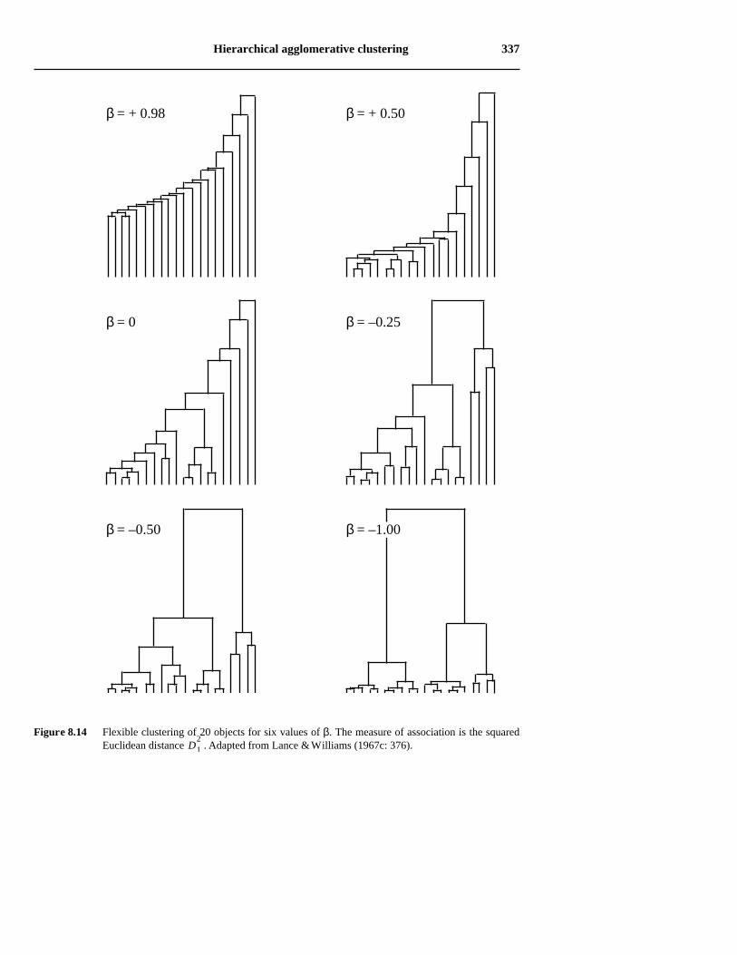
Hierarchical agglomerative clustering 337
Figure 8.14 Flexible clustering of 20 objects for six values of β. The measure of association is the squaredEuclidean distance . Adapted from Lance & Williams (1967c: 376).D1
2
β = –0.50 β = –1.00
β = + 0.98 β = + 0.50
β = –0.25β = 0
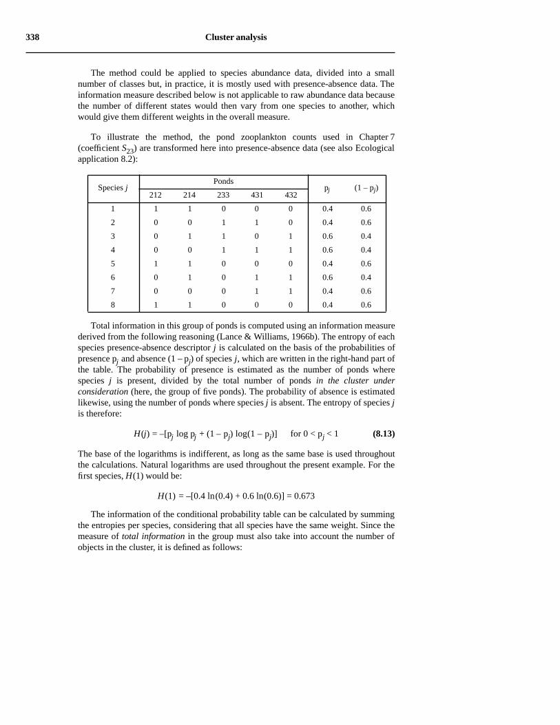
338 Cluster analysis
The method could be applied to species abundance data, divided into a smallnumber of classes but, in practice, it is mostly used with presence-absence data. Theinformation measure described below is not applicable to raw abundance data becausethe number of different states would then vary from one species to another, whichwould give them different weights in the overall measure.
To illustrate the method, the pond zooplankton counts used in Chapter 7(coefficient S23) are transformed here into presence-absence data (see also Ecologicalapplication 8.2):
Total information in this group of ponds is computed using an information measurederived from the following reasoning (Lance & Williams, 1966b). The entropy of eachspecies presence-absence descriptor j is calculated on the basis of the probabilities ofpresence pj and absence (1 – pj) of species j, which are written in the right-hand part ofthe table. The probability of presence is estimated as the number of ponds wherespecies j is present, divided by the total number of ponds in the cluster underconsideration (here, the group of five ponds). The probability of absence is estimatedlikewise, using the number of ponds where species j is absent. The entropy of species jis therefore:
H(j) = –[pj log pj + (1 – pj) log(1 – pj)] for 0 < pj < 1 (8.13)
The base of the logarithms is indifferent, as long as the same base is used throughoutthe calculations. Natural logarithms are used throughout the present example. For thefirst species, H(1) would be:
H(1) = –[0.4 ln(0.4) + 0.6 ln(0.6)] = 0.673
The information of the conditional probability table can be calculated by summingthe entropies per species, considering that all species have the same weight. Since themeasure of total information in the group must also take into account the number ofobjects in the cluster, it is defined as follows:
Species jPonds
pj (1 – pj)212 214 233 431 432
1 1 1 0 0 0 0.4 0.6
2 0 0 1 1 0 0.4 0.6
3 0 1 1 0 1 0.6 0.4
4 0 0 1 1 1 0.6 0.4
5 1 1 0 0 0 0.4 0.6
6 0 1 0 1 1 0.6 0.4
7 0 0 0 1 1 0.4 0.6
8 1 1 0 0 0 0.4 0.6
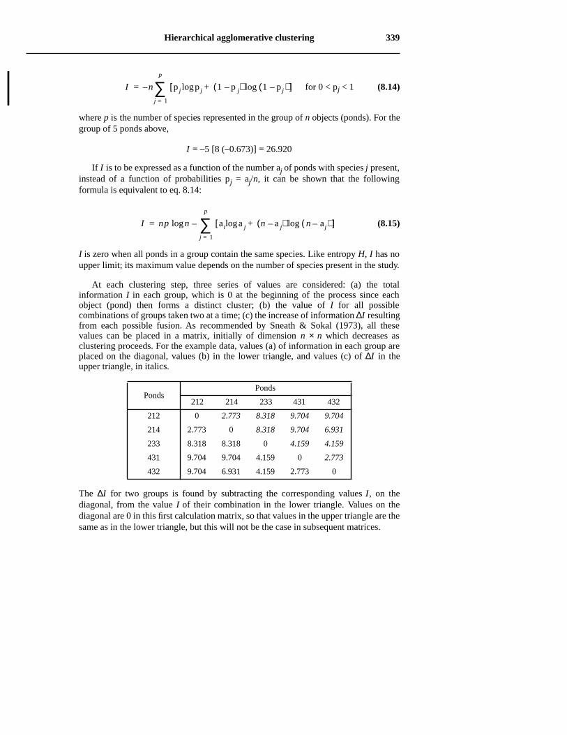
Hierarchical agglomerative clustering 339
for 0 < pj < 1 (8.14)
where p is the number of species represented in the group of n objects (ponds). For thegroup of 5 ponds above,
I = –5 [8 (–0.673)] = 26.920
If I is to be expressed as a function of the number aj of ponds with species j present,instead of a function of probabilities pj = aj/n, it can be shown that the followingformula is equivalent to eq. 8.14:
(8.15)
I is zero when all ponds in a group contain the same species. Like entropy H, I has noupper limit; its maximum value depends on the number of species present in the study.
At each clustering step, three series of values are considered: (a) the totalinformation I in each group, which is 0 at the beginning of the process since eachobject (pond) then forms a distinct cluster; (b) the value of I for all possiblecombinations of groups taken two at a time; (c) the increase of information ∆I resultingfrom each possible fusion. As recommended by Sneath & Sokal (1973), all thesevalues can be placed in a matrix, initially of dimension n × n which decreases asclustering proceeds. For the example data, values (a) of information in each group areplaced on the diagonal, values (b) in the lower triangle, and values (c) of ∆I in theupper triangle, in italics.
The ∆I for two groups is found by subtracting the corresponding values I, on thediagonal, from the value I of their combination in the lower triangle. Values on thediagonal are 0 in this first calculation matrix, so that values in the upper triangle are thesame as in the lower triangle, but this will not be the case in subsequent matrices.
PondsPonds
212 214 233 431 432
212 0 2.773 8.318 9.704 9.704
214 2.773 0 8.318 9.704 6.931
233 8.318 8.318 0 4.159 4.159
431 9.704 9.704 4.159 0 2.773
432 9.704 6.931 4.159 2.773 0
I n p j p jlog 1 p j–( ) 1 p j–( )log+[ ]j 1=
p
∑–=
I np n ai a jlog n a j–( ) n aj–( )log+[ ]j 1=
p
∑–log=
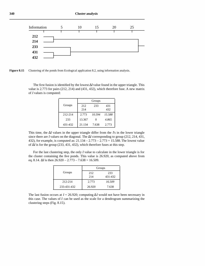
340 Cluster analysis
The first fusion is identified by the lowest ∆I value found in the upper triangle. Thisvalue is 2.773 for pairs (212, 214) and (431, 432), which therefore fuse. A new matrixof I values is computed:
This time, the ∆I values in the upper triangle differ from the I's in the lower trianglesince there are I values on the diagonal. The ∆I corresponding to group (212, 214, 431,432), for example, is computed as: 21.134 – 2.773 – 2.773 = 15.588. The lowest valueof ∆I is for the group (233, 431, 432), which therefore fuses at this step.
For the last clustering step, the only I value to calculate in the lower triangle is forthe cluster containing the five ponds. This value is 26.920, as computed above fromeq. 8.14. ∆I is then 26.920 – 2.773 – 7.638 = 16.509.
The last fusion occurs at I = 26.920; computing ∆I would not have been necessary inthis case. The values of I can be used as the scale for a dendrogram summarizing theclustering steps (Fig. 8.15).
Groups
Groups
212214
233 431432
212-214 2.773 10.594 15.588
233 13.367 0 4.865
431-432 21.134 7.638 2.773
Groups
Groups
212214
233431-432
212-214 2.773 16.509
233-431-432 26.920 7.638
Figure 8.15 Clustering of the ponds from Ecological application 8.2, using information analysis.
Information 5 10 15 20 25
212214233431432
Reversals 341
According to Williams et al. (1966), information analysis minimizes chaining andquickly delineates the main clusters, at least with ecological data. Field (1969) pointedout, however, that information analysis bases the similarity between objects on doubleabsences as well as double presences. This method may therefore not be appropriatewhen a gradient has been sampled and the data matrix contains many zeros; seeSection 7.3 and Subsection 9.4.5 for a discussion of this problem.
The inverse of ∆I is known as the efficiency coefficient (Lance & Williams, 1966b).An analogue to the efficiency coefficient may be computed for dendrograms obtainedusing other agglomerative clustering procedures. In that case, the efficiency coefficientis still computed as 1/∆, where ∆ represents the amount by which the information inthe classification is reduced due to the fusion of groups. The reduction is computed asthe entropy in the classification before a fusion level minus the entropy after thatfusion. In Fig. 8.2 for instance, the partition at S = 0.40 contains three groups of 2, 2,and 1 objects respectively; using natural logarithms, Shannon’s formula (eq. 6.1) givesH = 1.05492. The next partition, at S = 0.25, contains two groups of 2 and 3 objectsrespectively; Shannon’s formula gives H = 0.67301. The difference is ∆ = 0.38191,hence the efficiency coefficient 1/∆ = 2.61843 for the dendrogram fusion level S = 0.3.
When 1/∆I is high, the procedure clusters objects that are mostly alike. Theefficiency coefficient does not monotonically decrease as the clustering proceeds. Withreal data, it may decrease, reach a minimum, and increase again. If 1/∆I is plotted as afunction of the successive fusion levels, the minima in the graph indicate the mostimportant partitions. If one wants to select a single cutting level through a dendrogram,this graph may help in deciding which partition should be selected. In Fig. 8.2 forexample, one would choose the value 1/∆I = 1.48586, which corresponds to the lastfusion level (S = 0.214), as the most informative partition. The efficiency coefficient isnot a rigorous decision criterion, however, since no test of statistical significance isperformed.
8.6 Reversals
Reversals may occasionally occur in the clustering structure when using UPGMC orWPGMC (Subsections 8.5.6 and 8.5.7), or with some unusual combinations ofparameters in the general agglomerative model of Lance & Williams(Subsection 8.5.9). As an example, a reversal was produced in Fig. 8.7. Two types ofsituations lead to reversals:
• When x1 and x2 cluster first, because they represent the closest pair, although thedistance from x3 to the centroid c12 is smaller than the distance from x1 to x2(Fig. 8.16a).
Efficiencycoefficient
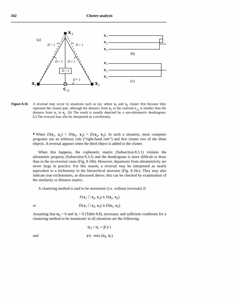
342 Cluster analysis
• When D(x1, x2) = D(x1, x3) = D(x2, x3). In such a situation, most computerprograms use an arbitrary rule (“right-hand rule”) and first cluster two of the threeobjects. A reversal appears when the third object is added to the cluster.
When this happens, the cophenetic matrix (Subsection 8.3.1) violates theultrametric property (Subsection 8.3.2) and the dendrogram is more difficult to drawthan in the no-reversal cases (Fig. 8.16b). However, departures from ultrametricity arenever large in practice. For this reason, a reversal may be interpreted as nearlyequivalent to a trichotomy in the hierarchical structure (Fig. 8.16c). They may alsoindicate true trichotomies, as discussed above; this can be checked by examination ofthe similarity or distance matrix.
A clustering method is said to be monotonic (i.e. without reversals) if:
S (x1 ∪ x2, x3) ≤ S (x1, x2)
or D(x1 ∪ x2, x3) ≥ D(x1, x2)
Assuming that αh > 0 and αi > 0 (Table 8.8), necessary and sufficient conditions for aclustering method to be monotonic in all situations are the following:
αh + α i + β ≥ 1
and γ ≥ –min (αh, αi)
Figure 8.16 A reversal may occur in situations such as (a), where x1 and x2 cluster first because theyrepresent the closest pair, although the distance from x3 to the centroid c12 is smaller than thedistance from x1 to x2. (b) The result is usually depicted by a non-ultrametric dendrogram.(c) The reversal may also be interpreted as a trichotomy.
x1 x2
x3
c12
D > 1
x 1
x 2
x 3
(a)
(b)
D > 1
D = 1
D = 1
D = 1
D < 1
x 1
x 2
x 3(c)
Hierarchical divisive clustering 343
(Milligan, 1979; Jain & Dubes, 1988). Some authors use the term classification onlyfor hierarchies without reversals or for single non-overlapping partitions of the objects(Section 8.8).
8.7 Hierarchical divisive clustering
Contrary to the agglomerative methods of Section 8.5, hierarchical divisive techniquesuse the whole set of objects as the starting point. They divide it into two or severalsubgroups, after which they consider each subgroup and divide it again, until thecriterion chosen to end the divisive procedure is met (Lance & Williams, 1967b).
In practice, hierarchical divisive clustering can only be achieved in the monotheticcase, or when working in an ordination space. In monothetic divisive methods, theobjects are divided, at each step of the procedure, according to the states of a singledescriptor. This descriptor is chosen because it best represents the whole set ofdescriptors (next subsection). Polythetic algorithms have been developed, but it will beseen that they are not satisfactory.
An alternative is to use a partitioning method (Section 8.8) for all possible numbersof groups from K = 2 to K = (n – 1) and assemble the results into a graph. There is noguarantee, however, that the groups will be nested and form a hierarchy, unless thebiological or ecological processes that have generated the data are themselveshierarchical.
1 — Monothetic methods
The clustering methods that use only one descriptor at a time are less than ideal, evenwhen the descriptor is chosen after considering all the others. The best-knownmonothetic method in ecology is Williams & Lambert's (1959) association analysis,originally described for species presence-absence data. Association analysis mayactually be applied to any binary data table, not only species. The problem is toidentify, at each step of the procedure, which descriptor is the most strongly associatedwith all the others. First, X2 (chi-square) values are computed for 2 × 2 contingencytables comparing all pairs of descriptors in turn. X2 is computed using the usualformula:
X2 = n (ad - bc)2/[(a + b) (c + d) (a + c) (b + d)]
The formula may include Yates’ correction for small sample sizes, as in similaritycoefficient S25. The X2 values relative to each descriptor k are summed up:
for j ≠ k (8.16)
Associationanalysis
X j k2
j 1=
p
∑
Partitioning by K-means 349
of selecting large gaps in the data, sites that may be very close in species compositionmay become separated.
There are other problems with TWINSPAN when it comes to identifying clusters ofspecies or computing indicator values.
• Firstly, when identifying clusters of species or computing indicator values, onecannot introduce some other classification of the sites in the program; only theclassifications produced by TWINSPAN, which are based on correspondence analysis(CA) or detrended correspondence analysis (DCA, Subsection 9.4.5), may be used todelineate species groups.
• Secondly, the pseudospecies concept is based on species relative abundances. Therelative abundance of a species depends on the absolute abundances of the otherspecies present at the site. Such relative frequencies may be highly biased whensampling or harvesting mobile organisms; all species are not sampled with the sameefficiency because of differences in behaviour. There is always a distortion betweenthe estimated (i.e. observed) and real relative frequencies of species at any given site.A species abundance value observed at a site should only be compared to abundancevalues for the same species at other sites.
• Finally, whereas simple CA is well suited for studying species abundances observedat several sites (ter Braak 1985), DCA has recently been severely criticized(Subsection 9.4.5). Jackson and Somers (1991b) have shown that results obtained withDCA vary depending on the number of segments used to remove the arch effect.Therefore, several runs with different numbers of segments must be done to find stablefactorial axes and interpretable results.
8.8 Partitioning by K-means
Partitioning consists in finding a single partition of a set of objects (Table 8.1). Jain &Dubes (1988) state the problem in the following terms: given n objects in ap–dimensional space, determine a partition of the objects into K groups, or clusters,such that the objects within each cluster are more similar to one another than to objectsin the other clusters. The number of groups, K, is determined by the user. This problemhas first been stated in statistical terms by Fisher (1958), who proposed solutions (withor without constraint of contiguity; see Sections 12.6 and 13.2) for a single variable.
The difficulty is to define what “more similar” means. Several criteria have beensuggested; they can be divided into global and local criteria. A global criterion wouldbe, for instance, to represent each cluster by a type-object (on a priori grounds, orusing the centroids of Subsections 8.5.6 and 8.5.7) and assign each object to thenearest type-object. A local criterion uses the local structure of the data to delineateclusters; groups are formed by identifying high-density regions in the data. The
350 Cluster analysis
K–means method, described in the next paragraphs, is the most commonly used of thelatter type.
In K-means, the objective function that the partition to discover should minimize isthe same as in Ward’s agglomerative clustering method (Subsection 8.5.8): the totalerror sum of squares ( , or TESS). The major problem encountered by thealgorithms is that the solution on which the computation eventually converges dependsto some extent on the initial positions of the centroids. This problem does not exist inWard’s method, which proceeds iteratively by hierarchical agglomeration. However,even though Ward’s algorithm guarantees that the increase in sum of squared errors( , eq. 8.8) is minimized at each step of the agglomeration (so that any order ofentry of the objects should lead to the same solution, except in cases of equal distanceswhere a “right-hand” programming rule may prevail), there is no guarantee that anygiven Ward’s partition is optimal in terms of the criterion — surprising at this mayseem. This same problem occurs with all stepwise statistical methods.
The problem of the final solution depending on the initial positions of the centroidsis known as the “local minimum” problem in algorithms. The concept is illustrated inFig. 8.17, by reference to a solution space. It may be explained as follows. Solutions tothe K-means problem are the different ways to partition n objects into, say, K = 4groups. If a single object is moved from one group to another, the corresponding twosolutions will have slightly different values for the criterion to be minimized ( ).Imagine that all possible solutions form a “space of solutions”. The different solutionscan be plotted as a graph with the criterion as the ordinate. It is not necessary toaccurately describe the abscissa to understand the concept; it would actually be amultidimensional space. A K-means algorithm starts at some position in this space, theinitial position being assigned by the user (see below). It then tries to navigate thespace to find the solution that minimizes the objective criterion ( ). The space ofsolutions is not smooth, however. It may contain local minima from which thealgorithm may be unable to escape. When this happens, the algorithm has not foundthe overall minimum and the partition is not optimal in terms of the objective criterion.
Several solutions may be used to help a K-means algorithm converge towards theoverall minimum of the objective criterion . They involve either selecting specificobjects as “group seeds” at the beginning of the run, or attributing the objects to the Kgroups in some special way. Here are some commonly-used approaches:
• Provide an initial configuration corresponding to an (ecological) hypothesis. Theidea is to start the algorithm in a position in the solution space which is, hopefully,close to the final solution sought. This ideal situation is seldom encountered in realstudies, however.
• Provide an initial configuration corresponding to the result of a hierarchicalclustering, obtained from a space-conserving method (Table 8.8). One simply choosesthe partition into K groups found on the dendrogram and lists the objects pertaining to
Objectivefunction
EK2
∆Ehi2
EK2
Localminimum
EK2
EK2
EK2
Overallminimum
EK2

Partitioning by K-means 351
each group. The K-means algorithm will then be asked to rearrange the groupmembership and look for a better overall solution (lower statistic).
• If the program allows it, select as “group seed”, for each of the K groups to bedelineated, some object located near the centroid of that group. For very largeproblems, Lance & Williams (1967d) suggested to use as starting point the result of ahierarchical clustering of a random subset of the objects, using as “group seeds” eitherthe centroids of K clusters, or objects located near these centroids.
• Attribute the objects at random to the various groups. All K-means computerprograms offer this option. Find a solution and note the value. It is possible, ofcourse, that the solution found corresponds to a local minimum of . So, repeat thewhole procedure a number of times (for example, 100 times), starting every time froma different random configuration. Retain the solution that minimizes the statistic.One is more confident that this solution corresponds to the overall minimum when thecorresponding value of is found several times across the runs.
Several algorithms have been proposed to solve the K–means problem, which isbut one of a family of problems known in computer sciences as the NP–complete or
Figure 8.17 K-means algorithms search the space of solutions, trying to find the overall minimum (arrow) ofthe objective criterion to be minimized, while avoiding local minima (troughs).
Solution space
Cri
teri
on to
be
min
imiz
ed
Overallminimum
Partitioningalgorithm
Distance matrixRaw data table or
EK2
EK2
EK2
EK2
EK2
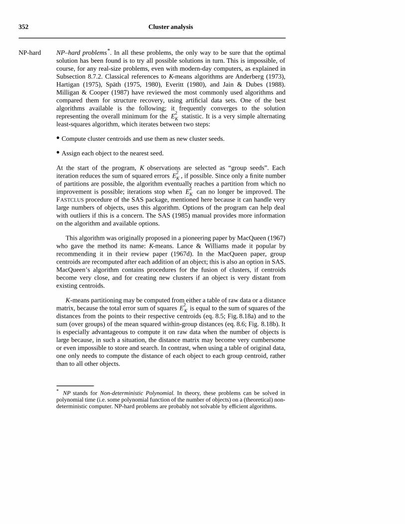
352 Cluster analysis
NP–hard problems*. In all these problems, the only way to be sure that the optimalsolution has been found is to try all possible solutions in turn. This is impossible, ofcourse, for any real-size problems, even with modern-day computers, as explained inSubsection 8.7.2. Classical references to K-means algorithms are Anderberg (1973),Hartigan (1975), Späth (1975, 1980), Everitt (1980), and Jain & Dubes (1988).Milligan & Cooper (1987) have reviewed the most commonly used algorithms andcompared them for structure recovery, using artificial data sets. One of the bestalgorithms available is the following; it frequently converges to the solutionrepresenting the overall minimum for the statistic. It is a very simple alternatingleast-squares algorithm, which iterates between two steps:
• Compute cluster centroids and use them as new cluster seeds.
• Assign each object to the nearest seed.
At the start of the program, K observations are selected as “group seeds”. Eachiteration reduces the sum of squared errors , if possible. Since only a finite numberof partitions are possible, the algorithm eventually reaches a partition from which noimprovement is possible; iterations stop when can no longer be improved. TheFASTCLUS procedure of the SAS package, mentioned here because it can handle verylarge numbers of objects, uses this algorithm. Options of the program can help dealwith outliers if this is a concern. The SAS (1985) manual provides more informationon the algorithm and available options.
This algorithm was originally proposed in a pioneering paper by MacQueen (1967)who gave the method its name: K-means. Lance & Williams made it popular byrecommending it in their review paper (1967d). In the MacQueen paper, groupcentroids are recomputed after each addition of an object; this is also an option in SAS.MacQueen’s algorithm contains procedures for the fusion of clusters, if centroidsbecome very close, and for creating new clusters if an object is very distant fromexisting centroids.
K-means partitioning may be computed from either a table of raw data or a distancematrix, because the total error sum of squares is equal to the sum of squares of thedistances from the points to their respective centroids (eq. 8.5; Fig. 8.18a) and to thesum (over groups) of the mean squared within-group distances (eq. 8.6; Fig. 8.18b). Itis especially advantageous to compute it on raw data when the number of objects islarge because, in such a situation, the distance matrix may become very cumbersomeor even impossible to store and search. In contrast, when using a table of original data,one only needs to compute the distance of each object to each group centroid, ratherthan to all other objects.
* NP stands for Non-deterministic Polynomial. In theory, these problems can be solved inpolynomial time (i.e. some polynomial function of the number of objects) on a (theoretical) non-deterministic computer. NP-hard problems are probably not solvable by efficient algorithms.
NP-hard
EK2
EK2
EK2
EK2
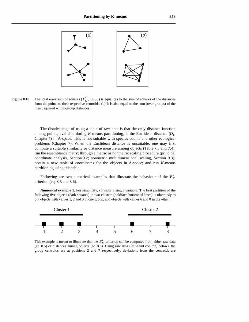
Partitioning by K-means 353
The disadvantage of using a table of raw data is that the only distance functionamong points, available during K-means partitioning, is the Euclidean distance (D1,Chapter 7) in A-space. This is not suitable with species counts and other ecologicalproblems (Chapter 7). When the Euclidean distance is unsuitable, one may firstcompute a suitable similarity or distance measure among objects (Table 7.3 and 7.4);run the resemblance matrix through a metric or nonmetric scaling procedure (principalcoordinate analysis, Section 9.2; nonmetric multidimensional scaling, Section 9.3);obtain a new table of coordinates for the objects in A-space; and run K-meanspartitioning using this table.
Following are two numerical examples that illustrate the behaviour of the criterion (eq. 8.5 and 8.6).
Numerical example 1. For simplicity, consider a single variable. The best partition of thefollowing five objects (dark squares) in two clusters (boldface horizontal lines) is obviously toput objects with values 1, 2 and 3 in one group, and objects with values 6 and 8 in the other:
This example is meant to illustrate that the criterion can be computed from either raw data(eq. 8.5) or distances among objects (eq. 8.6). Using raw data (left-hand column, below), thegroup centroids are at positions 2 and 7 respectively; deviations from the centroids are
Figure 8.18 The total error sum of squares ( , TESS) is equal (a) to the sum of squares of the distancesfrom the points to their respective centroids. (b) It is also equal to the sum (over groups) of themean squared within-group distances.
EK2
*
*
(a) (b)
EK2
1 2 3 4 5 6 7 8
Cluster 1 Cluster 2
EK2
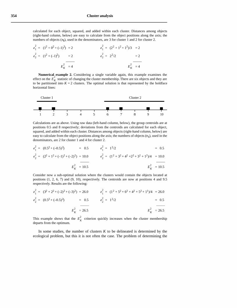
354 Cluster analysis
calculated for each object, squared, and added within each cluster. Distances among objects(right-hand column, below) are easy to calculate from the object positions along the axis; thenumbers of objects (nk), used in the denominators, are 3 for cluster 1 and 2 for cluster 2.
= (12 + 02 + (–1)2) = 2 = (22 + 12 + 12)/3 = 2
= (12 + (–1)2) = 2 = 22/2 = 2_____ _____
= 4 = 4
Numerical example 2. Considering a single variable again, this example examines theeffect on the statistic of changing the cluster membership. There are six objects and they areto be partitioned into K = 2 clusters. The optimal solution is that represented by the boldfacehorizontal lines:
Calculations are as above. Using raw data (left-hand column, below), the group centroids are atpositions 0.5 and 8 respectively; deviations from the centroids are calculated for each object,squared, and added within each cluster. Distances among objects (right-hand column, below) areeasy to calculate from the object positions along the axis; the numbers of objects (nk), used in thedenominators, are 2 for cluster 1 and 4 for cluster 2.
= (0.52 + (–0.5)2) = 0.5 = 12/2 = 0.5
= (22 + 12 + (–1)2 + (–2)2) = 10.0 = (12 + 32 + 42 +22 + 32 + 12)/4 = 10.0_____ _____
= 10.5 = 10.5
Consider now a sub-optimal solution where the clusters would contain the objects located atpositions (1, 2, 6, 7) and (9, 10), respectively. The centroids are now at positions 4 and 9.5respectively. Results are the following:
= (32 + 22 + (–2)2 + (–3)2) = 26.0 = (12 + 52 + 62 + 42 + 52 + 11)/4 = 26.0
= (0.52 + (–0.5)2) = 0.5 = 12/2 = 0.5_____ _____
= 26.5 = 26.5
This example shows that the criterion quickly increases when the cluster membershipdeparts from the optimum.
In some studies, the number of clusters K to be delineated is determined by theecological problem, but this it is not often the case. The problem of determining the
e12
e12
e22
e22
EK2
EK2
EK2
1 2 3 4 5 6 7 8 9
Cluster 1
10
Cluster 2
e12
e12
e22
e22
EK2
EK2
e12
e12
e22
e22
EK2
EK2
EK2

Species clustering: biological associations 355
most appropriate number of clusters has been extensively discussed in the literature.Over 30 different methods, called “stopping rules”, have been proposed to do so. Theefficiency coefficient, described in the last paragraph of Section 8.5, is one of them.Milligan & Cooper (1985; see also Milligan, 1996) compared them through anextensive series of simulations using artificial data sets with known numbers ofclusters. Some of these rules recover the correct number of clusters in most instances,but others are appallingly inefficient. SAS, for instance, has implemented two amongthe best of these rules: a pseudo-F statistic and the cubic clustering criterion.
8.9 Species clustering: biological associations
Most of the methods discussed in the previous sections may be applied to clusteringdescriptors as well as objects. When searching for species associations, however, it isimportant to use clustering methods that model as precisely as possible a clearlyformulated concept of association. The present section attempts (1) to define anoperational concept of association and (2) to show how species associations can beidentified in that framework.
Several concepts of species association have been developed since the nineteenthcentury; Whittaker (1962) wrote a remarkable review about them. These concepts arenot always operational, however. In other words, they cannot always be translated intoa series of well-defined analytical steps which would lead to the same result if theywere applied by two independent researchers, using the same data. In general, theconcept of association refers to a group of species that are “significantly” foundtogether, without this implying necessarily any positive interaction among thesespecies. In other words, an association is simply a group of species (or of taxapertaining to some systematic category) recognized as a cluster following theapplication of a clearly stated set of rules.
Several procedures have been proposed for the identification of speciesassociations. Quantitative algorithms have progressively replaced the empiricalmethods, as they have in other areas of science. All these methods, whether simple orelaborate, have two goals: first, identify the species that occur together and, second,minimize the likelihood that the co-occurrences so identified be fortuitous. The searchfor valid associations obviously implies that the sampling be random and planned inaccordance with the pattern of variability under study (e.g. geographical, temporal,vertical, experimental). This pattern defines the framework within which the groups ofspecies, found repeatedly along the sampling axes, are called associations; one thenspeaks of association of species over geographic space, or in time, etc. The criterion isthe recurrence of a group of species along the sampling axes under study.
Ecologists are interested in associations of species as a conceptual framework tosynthesize environmental characteristics. When associations have been found, one canconcentrate on finding the ecological requirements common to most or all species of