Chapter 7b Polarization Curve...
33
Chapter 7b Polarization Curve Applications Introduction In this chapter, we will continue to explore features of the OLI Studio: Corrosion Analyzer specifically looking at corrosion rates and polarization curves with practical examples. Sections 7b.1 Corrosion in a Water-Filled Carbon Steel Tank ..........................................................................................2 7b.2 Corrosion in a Pipe Carrying Acids ........................................................................................................... 10 7b.3 Corrosivity of Soda Pop ........................................................................................................................... 15 7b.4 Corrosion of Steel Pilings in Seawater ..................................................................................................... 18 7b.5 Gas Condensate Corrosion ...................................................................................................................... 24
Transcript of Chapter 7b Polarization Curve...

Chapter 7b Polarization Curve Applications
Introduction
In this chapter, we will continue to explore features of the OLI Studio: Corrosion Analyzer specifically looking at corrosion rates and polarization curves with practical examples.
Sections 7b.1 Corrosion in a Water-Filled Carbon Steel Tank ..........................................................................................2
7b.2 Corrosion in a Pipe Carrying Acids ........................................................................................................... 10
7b.3 Corrosivity of Soda Pop ........................................................................................................................... 15
7b.4 Corrosion of Steel Pilings in Seawater ..................................................................................................... 18
7b.5 Gas Condensate Corrosion ...................................................................................................................... 24
7b-2 Chapter 7b: Polarization Curve Applications Tricks of the Trade
7b.1 Corrosion in a Water-Filled Carbon Steel Tank
Overview
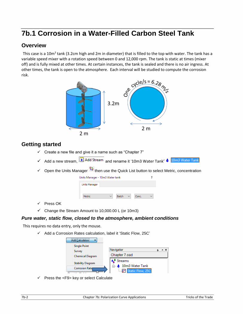
This case is a 10m3 tank (3.2cm high and 2m in diameter) that is filled to the top with water. The tank has a variable speed mixer with a rotation speed between 0 and 12,000 rpm. The tank is static at times (mixer off) and is fully mixed at other times. At certain instances, the tank is sealed and there is no air ingress. At other times, the tank is open to the atmosphere. Each interval will be studied to compute the corrosion risk.
Getting started
✓ Create a new file and give it a name such as “Chapter 7”
✓ Add a new stream, and rename it ‘10m3 Water Tank’
✓ Open the Units Manager then use the Quick List button to select Metric, concentration
✓ Press OK
✓ Change the Stream Amount to 10,000.00 L (or 10m3)
Pure water, static flow, closed to the atmosphere, ambient conditions
This requires no data entry, only the mouse.
✓ Add a Corrosion Rates calculation, label it ‘Static Flow, 25C’
✓ Press the <F9> key or select Calculate

Tricks of the Trade Chapter 7b: Polarization Curve Applications 7b-3
✓ Click on the “1” tab at the bottom of the grid
The Corrosion Rate is 7.1e-3 mm/yr. This is a negligible rate, for if the tank wall’s thickness is ½ inch (~12.7 mm) then corroding half the wall thickness would take about 900 years.
Pure water, turbulent flow, closed to the atmosphere, ambient conditions
✓ Add a nerw Corrosion Rates and rename it ‘Turbulent Flow, 25C’
✓ Select on the Static cell in the Flow Type and change to Complete Agitation
✓ Calculate
✓ Select the “1” tab at the bottom of the grid

7b-4 Chapter 7b: Polarization Curve Applications Tricks of the Trade
The corrosion rate increased 0.019 mm/yr, still a relatively low value.
Pure water, varying flow, closed to the atmosphere, ambient conditions
The next step is to compute the flow across the tank wall. The software contains four flow types, Pipe, Disk, Cylinder, and Shear Stress. The best option is probably the Rotating Cylinder, which would be the tank moving relative to the water.
✓ Add a new Corrosion Rates and rename it ‘Varying Flow, 25C’
✓ Change the Survey by to Rotating Cylinder
✓ Change the Rotor diameter to 200 cm
The vertical dimensions of the tank are unimportant. We will assume that the tank can be modeled like a rotating cylinder. The propeller rotates at 1200 rpm, although it is not expected that the wall velocity w will approach this value, and so a lower value will be used (we still want it to be high enough to see the effects of shear). The next step is to set the speed of the mixer.
✓ Select the Specs button.

Tricks of the Trade Chapter 7b: Polarization Curve Applications 7b-5
Varying Flow, 25C Survey Range
Start 0
End 300
Increment 10
✓ In Var1 – Rotator Rotation category, change the Survey Range according to the table above
✓ Press OK then Calculate
✓ Select the General Corr. Rate tab then select the Curves button
✓ Double-click pH-Aqueous in the Y2 Axis to remove it
✓ Press OK then view the plot
The corrosion rate is computed to increase as the bulk liquid velocity increases from 0 to 300 rpm near the wall surface. The reason is straightforward; The higher velocity reduces the static water film thickness on the metal surface. This Diffusion Layer film limits the mass transfer of corrosion products and bulk chemicals to and from the surface. As the liquid velocity (and therefore shear force) increases, the film thickness decreases, and the concentration gradient increase. This increases the flux of materials to and from the surface, which increase corrosion rates.
7b-6 Chapter 7b: Polarization Curve Applications Tricks of the Trade
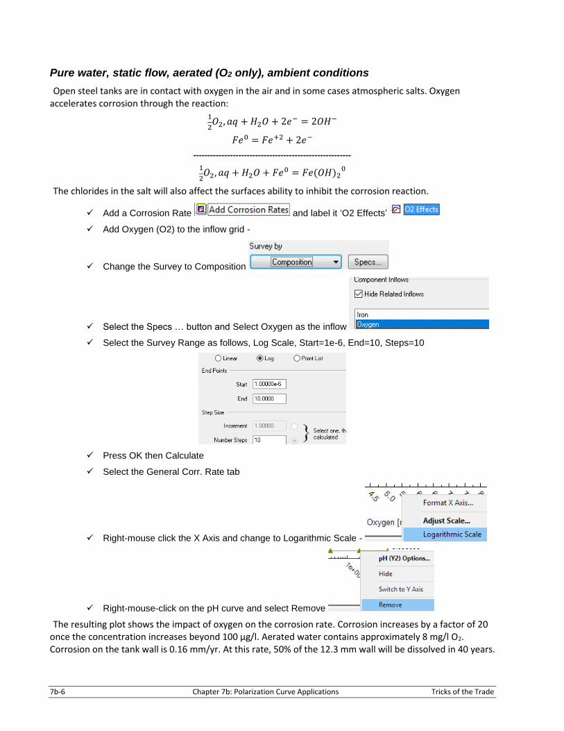
Pure water, static flow, aerated (O2 only), ambient conditions
Open steel tanks are in contact with oxygen in the air and in some cases atmospheric salts. Oxygen accelerates corrosion through the reaction:
1
2𝑂2, 𝑎𝑞 + 𝐻2𝑂 + 2𝑒− = 2𝑂𝐻−
𝐹𝑒0 = 𝐹𝑒+2 + 2𝑒−
--------------------------------------------------------
1
2𝑂2, 𝑎𝑞 + 𝐻2𝑂 + 𝐹𝑒0 = 𝐹𝑒(𝑂𝐻)2
0
The chlorides in the salt will also affect the surfaces ability to inhibit the corrosion reaction.
✓ Add a Corrosion Rate and label it ‘O2 Effects’
✓ Add Oxygen (O2) to the inflow grid -
✓ Change the Survey to Composition
✓ Select the Specs … button and Select Oxygen as the inflow
✓ Select the Survey Range as follows, Log Scale, Start=1e-6, End=10, Steps=10
✓ Press OK then Calculate
✓ Select the General Corr. Rate tab
✓ Right-mouse click the X Axis and change to Logarithmic Scale -
✓ Right-mouse-click on the pH curve and select Remove
The resulting plot shows the impact of oxygen on the corrosion rate. Corrosion increases by a factor of 20 once the concentration increases beyond 100 µg/l. Aerated water contains approximately 8 mg/l O2. Corrosion on the tank wall is 0.16 mm/yr. At this rate, 50% of the 12.3 mm wall will be dissolved in 40 years.

Tricks of the Trade Chapter 7b: Polarization Curve Applications 7b-7
Air also contains carbon dioxide, which will corrode steel. Its impact is studied in the next calculation.
Pure water, static flow, aerated (O2, CO2), ambient conditions
The atmosphere contains ~400 ppmV CO2. At this concentration 0.6 mg/l CO2 is dissolved in water as molecular CO2, this CO2 hydrolyzes (splits) water to form the following reactants.
𝐶𝑂2 + 𝐻2𝑂 = 𝐻+ + 𝐻𝐶𝑂3−
The resulting pH is about 5.6 at ambient conditions.
The impact of CO2 on corrosion is two-fold, as two separate reactions occur at the metal surface
𝐻+ + 𝑒− =1
2𝐻2
𝐻𝐶𝑂3− + 𝑒− =
1
2𝐻2 + 𝐶𝑂3
−2
To test the CO2 impact, you will recalculate the corrosion rate using two CO2 concentrations: 0 and 0.6 ppm.
✓ Copy the existing O2 effects calculation and paste it back to the 10 m3 Water Tank stream.
o Right-mouse click on the calculation and select Copy
o Right-mouse click the 10 m3 Aerated Water Tank, and select Paste
✓ Rename the duplicated object ‘CO2 Effects’
✓ Change the Names Manager to Formula view -
✓ Add O2 and CO2 to the Inflow grid (the O2 may not have copied over)
✓ Change the Then By (optional) option from None to Composition
7b-8 Chapter 7b: Polarization Curve Applications Tricks of the Trade
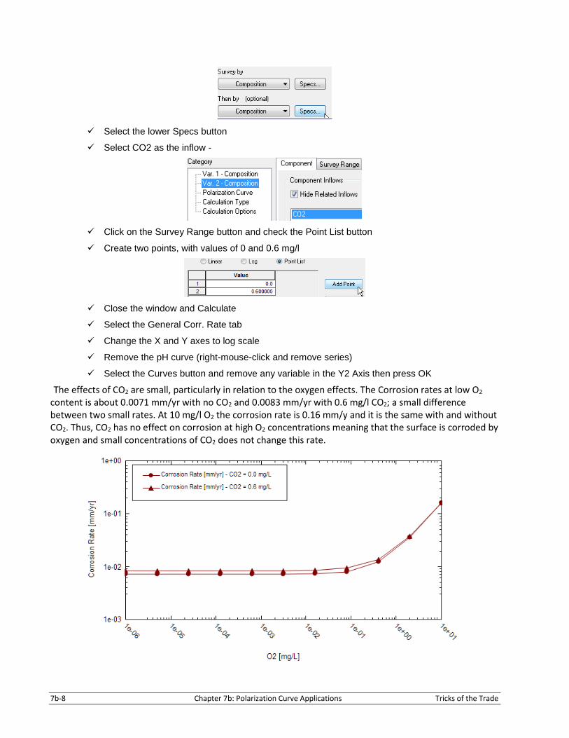
✓ Select the lower Specs button
✓ Select CO2 as the inflow -
✓ Click on the Survey Range button and check the Point List button
✓ Create two points, with values of 0 and 0.6 mg/l
✓ Close the window and Calculate
✓ Select the General Corr. Rate tab
✓ Change the X and Y axes to log scale
✓ Remove the pH curve (right-mouse-click and remove series)
✓ Select the Curves button and remove any variable in the Y2 Axis then press OK
The effects of CO2 are small, particularly in relation to the oxygen effects. The Corrosion rates at low O2 content is about 0.0071 mm/yr with no CO2 and 0.0083 mm/yr with 0.6 mg/l CO2; a small difference between two small rates. At 10 mg/l O2 the corrosion rate is 0.16 mm/y and it is the same with and without CO2. Thus, CO2 has no effect on corrosion at high O2 concentrations meaning that the surface is corroded by oxygen and small concentrations of CO2 does not change this rate.

Tricks of the Trade Chapter 7b: Polarization Curve Applications 7b-9
Pure water, 300 cycles/min flow, aerated (O2, CO2), ambient conditions
Lastly, you will look at the effects of shear rates on the tank in contact with CO2 and O2.
✓ Select the Definition tab
✓ Change the Flow type from Static to Rotating Cylinder
✓ Set the Rotor Diameter to 200 cm
✓ Set the Rotor Rotation to 300 cycles/minute
✓ Calculate then select the General Corr. Rate tab to review the plot
The 0.6 mg/l CO2 curves shifted at low O2 concentrations. The rate is 0.048 mm/yr compared to 0.008 mm/yr at static conditions. The effect of shear at high O2 concentrations (right side of the plot) is also pronounced. Corrosion is still dominated by O2 attack, but the rate is now over 10 mm/yr. about 100x greater than the static conditions.
✓ Save the file

7b-10 Chapter 7b: Polarization Curve Applications Tricks of the Trade
7b.2 Corrosion in a Pipe Carrying Acids Some of the more common commercial acids include muriatic acid (20% HCl), Aqua Regia (25% HNO3:75%
HCl), Battery Acid (30% H2SO4), commercial grade nitric acid (68% HNO3), and fuming HCl (37%).
In this example, the metallurgy within a vacuum HCl tower will be studied.at HCl production. Fuming HCl is purified from feedstock through distillation. The HCl-H2O mixture however, forms an Azeotrope at 20% HCl and 110C. Consequently, multiple distillation sequences are needed to achieve the 37% mixture. In this case, the conditions within the first towe are investigated. Here the feedstock is at vacuum pressures (0.3 atm).
Vacuum HCL Tower
Stage T, C HCl % H2O %
1 78.1 25 75
2 77.6 24 76
3 77 23 77
4 76.3 22 78
5 75.4 21 79
6 74.4 20 80
7 73.6 20 80
8 72.8 19 81
9 68.7 12 88
Carbon steel tower
✓ Add a new stream ; rename it ‘Vacuum HCl Tower’
✓ Open the Units Manager then use the Quick List button to select Metric, Flowing, Mass Fraction
✓ Set the Stream Amount to 12500 kg/hr
The Stream Amount does not have to be changed, but to keep this stream consistent with the process, the conditions and compositions will be included.
✓ Change the pressure to 0.3 atm
This is the tower pressure, which in fact decreases from 0.3 to 0.25 atm (bottom to top of tower). However, it is not practical to adjust the pressure when changing temperature and HCl% content, so we will leave the value at the tower bottom pressure
✓ In the Inflows grid, enter HCl
✓ Add a Corrosion Rate calculation and name it Carbon Steel -
✓ Change the Survey by to Temperature
✓ Change the Then by (optional) to Composition
✓ Select the Together button just above the Calculate button
✓ Select the top Specs button

Tricks of the Trade Chapter 7b: Polarization Curve Applications 7b-11
✓ Click the Point List button
✓ Create nine points and enter the temperatures from the table above
✓ Click on the Var. 2 Composition Category and select HCl as the inflow to be adjusted
✓ Click the Survey Range tab and click on the Point List button
✓ Add eight more points to the list and enter the %HCl values from the table above

7b-12 Chapter 7b: Polarization Curve Applications Tricks of the Trade
✓ Press OK then Calculate
✓ Select General Corr. Tab
✓ Remove the pH curve – Right-mouse-click and select Remove
Corrosion rates increase from 270 mm/yr at the top of the tower to 2760 mm/yr at the bottom. At these rates, the 1” thick (254 mm) carbon steel plate at the tower bottom will dissolve in about 30 hours!
Another material of construction is needed. We will test these out now.
316 stainless steel tower
✓ Copy the Carbon Steel corrosion calculation and paste it twice to the Vacuum HCl Tower
✓ Name the new calculation Stainless Steel 316 -

Tricks of the Trade Chapter 7b: Polarization Curve Applications 7b-13
✓ Change the Contact Surface to Stainless Steel 316
✓ Calculate then select the General Corr. Tab
✓ Remove the pH
The Corrosion rates for 316 stainless are about 10 times lower than carbon steel. The rates vary from 22 at the tower top to 310 mm/yr at its bottom. This is still a very high value, as a 254 mm wall at the tower bottom would dissolve in nine months.
Corrosion using a Duplex Stainless 2205 (high chrome)
✓ Rename the third calculation object Duplex 2205 (copied)

7b-14 Chapter 7b: Polarization Curve Applications Tricks of the Trade
✓ Change the Contact Surface to Duplex Stainless 2205 -
✓ Calculate then select the General Corr. Tab
Corrosion rates are considerably smaller, one-thousandth the rates observed with carbon steel and up to 100 times less than 316 stainless.
At these rates, which are roughly the same across the tower (1.1 to 1.26 mm/yr), a 25 mm duplex steel wall will lose one-half its wall thickness in 20 years.
Tricks of the Trade Chapter 7b: Polarization Curve Applications 7b-15
7b.3 Corrosivity of Soda Pop In this example, you will compute the corrosion rate of soda on an aluminum can. Aluminum cans are
internally coated with an epoxy resin to prevent corrosion.1 In this exercise, you will compute the corrosion rate without this coating Below are some properties for various soda brands. These soda products contain phosphoric or citric acid and is pressure is carbonation (CO2), this produces a low pH.
You will create soda properties by adding H3PO4 to lower pH and CO2 to raise the bubble point pressure. You will then compute the corrosivity of this liquid on aluminum. You can alternatively test the effects of citric acid on corrosivity, and figure out how much tooth enamel (calcium flurophosphate) will dissolve in 12 ounces (355 ml) of soda.
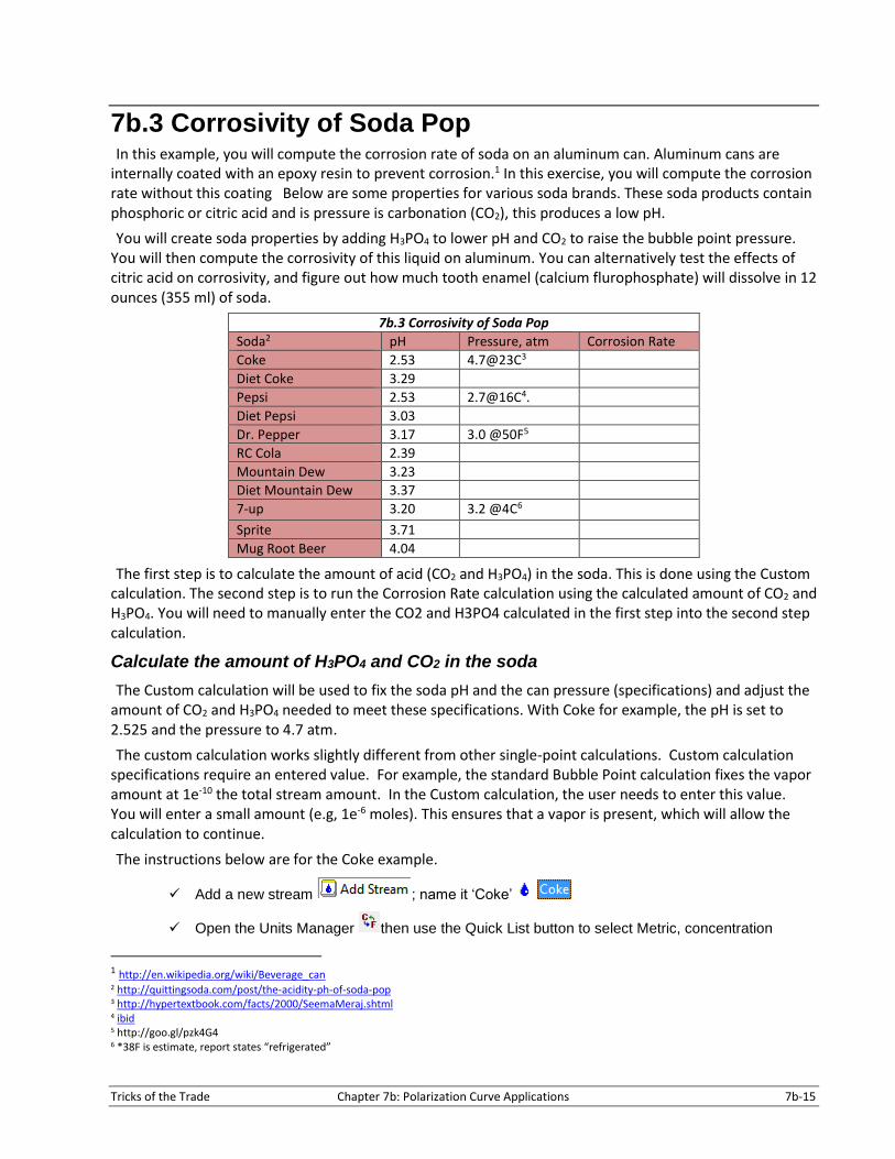
7b.3 Corrosivity of Soda Pop
Soda2 pH Pressure, atm Corrosion Rate
Coke 2.53 4.7@23C3
Diet Coke 3.29
Pepsi 2.53 2.7@16C4.
Diet Pepsi 3.03
Dr. Pepper 3.17 3.0 @50F5
RC Cola 2.39
Mountain Dew 3.23
Diet Mountain Dew 3.37
7-up 3.20 3.2 @4C6
Sprite 3.71
Mug Root Beer 4.04
The first step is to calculate the amount of acid (CO2 and H3PO4) in the soda. This is done using the Custom calculation. The second step is to run the Corrosion Rate calculation using the calculated amount of CO2 and H3PO4. You will need to manually enter the CO2 and H3PO4 calculated in the first step into the second step calculation.
Calculate the amount of H3PO4 and CO2 in the soda
The Custom calculation will be used to fix the soda pH and the can pressure (specifications) and adjust the amount of CO2 and H3PO4 needed to meet these specifications. With Coke for example, the pH is set to 2.525 and the pressure to 4.7 atm.
The custom calculation works slightly different from other single-point calculations. Custom calculation specifications require an entered value. For example, the standard Bubble Point calculation fixes the vapor amount at 1e-10 the total stream amount. In the Custom calculation, the user needs to enter this value. You will enter a small amount (e.g, 1e-6 moles). This ensures that a vapor is present, which will allow the calculation to continue.
The instructions below are for the Coke example.
✓ Add a new stream ; name it ‘Coke’
✓ Open the Units Manager then use the Quick List button to select Metric, concentration
1 http://en.wikipedia.org/wiki/Beverage_can 2 http://quittingsoda.com/post/the-acidity-ph-of-soda-pop 3 http://hypertextbook.com/facts/2000/SeemaMeraj.shtml 4 ibid 5 http://goo.gl/pzk4G4 6 *38F is estimate, report states “refrigerated”

7b-16 Chapter 7b: Polarization Curve Applications Tricks of the Trade
✓ Add H3PO4 and CO2 to the grid
✓ Change the Stream amount to 0.355 L (12 ounces)
✓ Change the temperature to 23C
✓ Change the pressure to 4.7 atm
✓ Add a Single Point calculation then change the type to Custom
✓ Select the Specs button
✓ Open the Specs window
✓ In the Variables to Fix column, select Moles (True)-Vapor and pH
✓ In the Variables to Free column, select CO2 and H3PO4
✓ Press OK
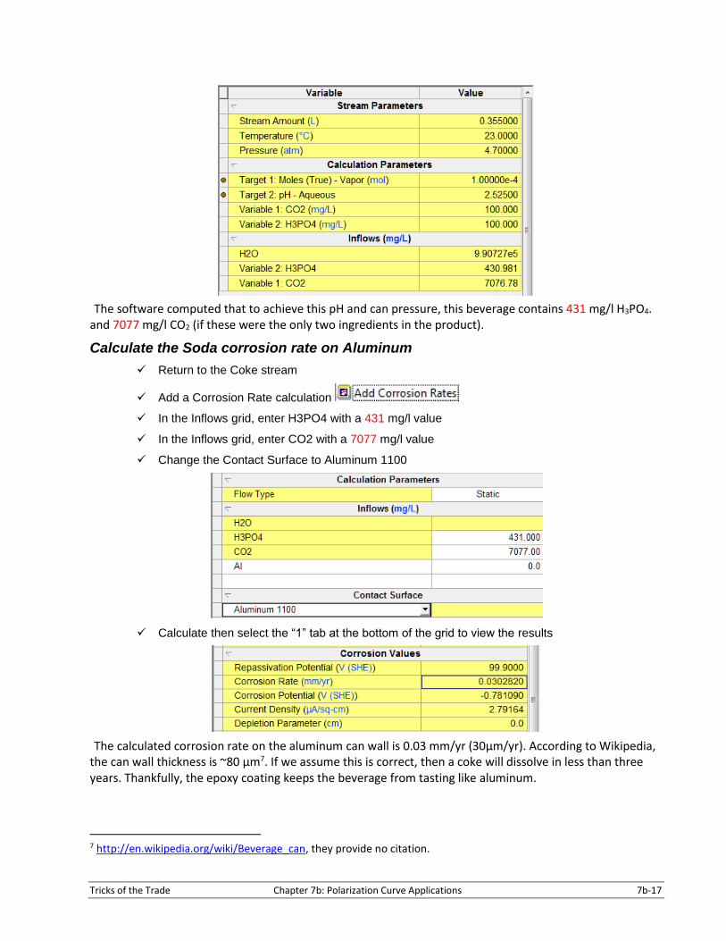
The Calculation Parameters Section of the grid is active and it contains four rows, two target specifications and two adjustable variables. The Target specifications require values. The adjustable variables can benefit from adding initial guesses, since it can speed up the calculation. You will add initial guesses in this case.
✓ Add the following Values to the Calculation Parameters Section
7b.3 Calculation Parameters
Target 1: Moles - Vapor 1e-4
Target 2: pH – Aqueous 2.525
Variable 1: CO2 (mg/l) 100
Variable 2: H3PO4 (mg/l) 100
✓ Calculate
✓ Click on the Output tab at the bottom of the grid
Tricks of the Trade Chapter 7b: Polarization Curve Applications 7b-17
The software computed that to achieve this pH and can pressure, this beverage contains 431 mg/l H3PO4. and 7077 mg/l CO2 (if these were the only two ingredients in the product).
Calculate the Soda corrosion rate on Aluminum
✓ Return to the Coke stream
✓ Add a Corrosion Rate calculation
✓ In the Inflows grid, enter H3PO4 with a 431 mg/l value
✓ In the Inflows grid, enter CO2 with a 7077 mg/l value
✓ Change the Contact Surface to Aluminum 1100
✓ Calculate then select the “1” tab at the bottom of the grid to view the results
The calculated corrosion rate on the aluminum can wall is 0.03 mm/yr (30µm/yr). According to Wikipedia, the can wall thickness is ~80 µm7. If we assume this is correct, then a coke will dissolve in less than three years. Thankfully, the epoxy coating keeps the beverage from tasting like aluminum.
7 http://en.wikipedia.org/wiki/Beverage_can, they provide no citation.
7b-18 Chapter 7b: Polarization Curve Applications Tricks of the Trade
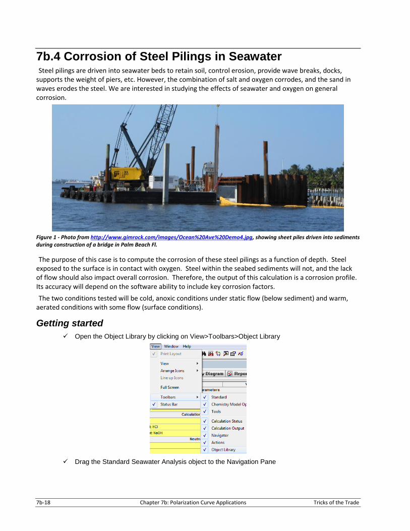
7b.4 Corrosion of Steel Pilings in Seawater Steel pilings are driven into seawater beds to retain soil, control erosion, provide wave breaks, docks,
supports the weight of piers, etc. However, the combination of salt and oxygen corrodes, and the sand in waves erodes the steel. We are interested in studying the effects of seawater and oxygen on general corrosion.
Figure 1 - Photo from http://www.gimrock.com/images/Ocean%20Ave%20Demo4.jpg, showing sheet piles driven into sediments during construction of a bridge in Palm Beach Fl.
The purpose of this case is to compute the corrosion of these steel pilings as a function of depth. Steel exposed to the surface is in contact with oxygen. Steel within the seabed sediments will not, and the lack of flow should also impact overall corrosion. Therefore, the output of this calculation is a corrosion profile. Its accuracy will depend on the software ability to include key corrosion factors.
The two conditions tested will be cold, anoxic conditions under static flow (below sediment) and warm, aerated conditions with some flow (surface conditions).
Getting started
✓ Open the Object Library by clicking on View>Toolbars>Object Library
✓ Drag the Standard Seawater Analysis object to the Navigation Pane
Tricks of the Trade Chapter 7b: Polarization Curve Applications 7b-19
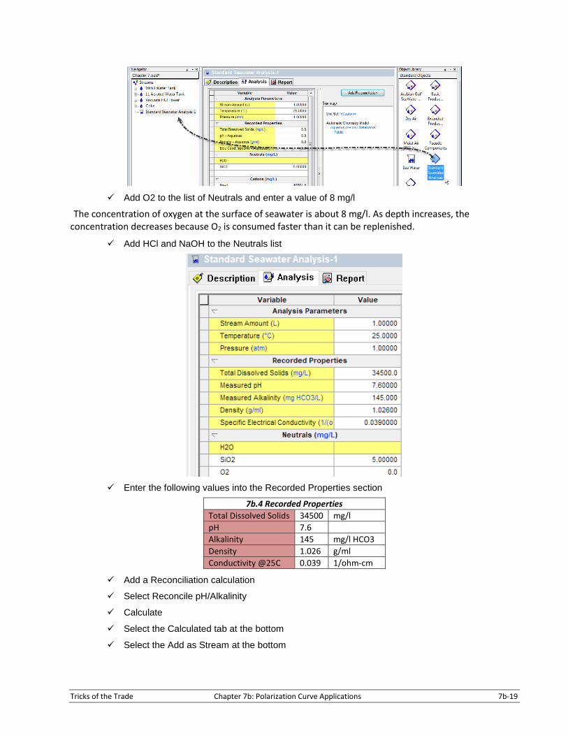
✓ Add O2 to the list of Neutrals and enter a value of 8 mg/l
The concentration of oxygen at the surface of seawater is about 8 mg/l. As depth increases, the concentration decreases because O2 is consumed faster than it can be replenished.
✓ Add HCl and NaOH to the Neutrals list
✓ Enter the following values into the Recorded Properties section
7b.4 Recorded Properties
Total Dissolved Solids 34500 mg/l
pH 7.6
Alkalinity 145 mg/l HCO3
Density 1.026 g/ml
Conductivity @25C 0.039 1/ohm-cm
✓ Add a Reconciliation calculation
✓ Select Reconcile pH/Alkalinity
✓ Calculate
✓ Select the Calculated tab at the bottom
✓ Select the Add as Stream at the bottom

7b-20 Chapter 7b: Polarization Curve Applications Tricks of the Trade
✓ Name the Exported stream Seawater and press OK
This creates a new stream called Seawater. This stream contains the molecular composition of the analysis we reconciled. Converting the water analysis to a stream format makes available the standard calculation objects, like Single Point, Survey, Corrosion Rates.
Corrosion between 10 and 30 C and in static flow
The first scenario is to compute the general corrosion rate as temperature changes. Seawater temperature varies with location (near shore, offshore), depth, latitude, and season. In our case, we are interested in near-shore water, perhaps 10 meters deep, where the water temperature range is 10 to 30 C.
✓ Add a Corrosion Rate Calculation to this new stream
✓ Change the Survey by to Temperature
✓ Open the Specs window and set the Start=10, End=30, and Increment=1 C
✓
✓ Press OK and Calculate
✓ Select the General Corr. Rate tab then the Curves button
✓ Remove the pH from the plot using the right-mouse-click option.

Tricks of the Trade Chapter 7b: Polarization Curve Applications 7b-21
The corrosion rates vary range from 0.080 to 0.140 mm/yr under static conditions. Notice that a few of the calculations failed (the zero values). Calculation failures occur at time, and when it does, ignore the values if we can as long as it does not detract from the interpretation. With respect to the corrosion rate, a steel pilings 12.7 mm thick will last up to 80 years (50% wall loss).
Corrosion between 10 and 30C in liquid flowing
If the water is flowing, then the situation is different. Modeling waves moving against the pilings is not simple, and there is no Flow Type (flow model) in the software that mimics it. We can attempt a guess.
We assume that the water flows across the surface at a rate at which a person walks, ~5 km/hr. This is about 1.5 m/s. Next, we need to consider the shape of the surface. The software does not have a flat plate, but perhaps a pipe with a large diameter would suffice. We can try several diameters, 1.000 or 10,000 meters for example (the arc would approach a flat plate).
✓ Return to the Definition tab
✓ Change the flow type to Pipe Flow
✓ Change the Pipe Diameter units to meters
✓ Set the pipe diameter to 10000 meters
✓ Change the Pipe Flow Velocity to 1.5 m/s
✓ Calculate and View the Plot
The corrosion rate increases by a factor of 10x, decreasing the piling life to about 8-10 years.

7b-22 Chapter 7b: Polarization Curve Applications Tricks of the Trade
Compare to Field Data8
An NBS monograph written in 1977 provides some reference for our evaluation. The adjacent plot contains the wall loss on unlined steel pilings driven into the soil. A portion of the pipe is exposed to wave action, tide changes, sand movement, and quiescent pore waters.
The mean seawater salinity is 26.8 ppt, lower than the 34.5 g/l value used in our calculation. In addition, the mean sweater temperature is 14.4C
The piles are 30’ long (9.1m) and 0.7” (18mm) thick. They were driven into the sand to 19 ft. The wall loss occurs on two sides of the pilings. Therefore the wall loss is effectively double the corrosion rate.
The pilings were exposed to this environment for six years. They were inspected annually using electrochemical and visual methods. They were removed after six years for inspection.
The authors reported several distinct corrosion sections, from below the mud line to the splash and atmospheric section (adjacent plot). The highest corrosion was above the Mean High water, where corrosion rates were between 8 to 12 mpy.
Below the high water mark, the corrosion was between 4 and 8 mpy on average. At the Mudline, which is the erosion zone, the rate averaged 9 mpy, and shifted because of the shifting mud-line elevation.
8 Escalante, E.; Iverson, W. P.; Gerhold, W. F.; Sanderson, B. T. & Alumbaugh.1977. Corrosion and Protection of Steel
Piles in a Natural Seawater Environment. Washington D.C.. UNT Digital Library. http://digital.library.unt.edu/ark:/67531/metadc13190/.
Tricks of the Trade Chapter 7b: Polarization Curve Applications 7b-23
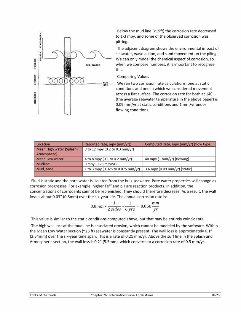
Below the mud line (<15ft) the corrosion rate decreased to 1-3 mpy, and some of the observed corrosion was pitting.
The adjacent diagram shows the environmental impact of seawater, wave action, and sand movement on the piling. We can only model the chemical aspect of corrosion, so when we compare numbers, it is important to recognize this.
Comparing Values
We ran two corrosion rate calculations, one at static conditions and one in which we considered movement across a flat surface. The corrosion rate for both at 14C (the average seawater temperature in the above paper) is 0.09 mm/yr at static conditions and 1 mm/yr under flowing conditions.
Location Reported rate, mpy (mm/yr)) Computed Rate, mpy (mm/yr) [flow type]
Mean High water (Splash-Atmosphere)
8 to 12 mpy (0.2 to 0.3 mm/yr)
Mean Low water 4 to 8 mpy (0.1 to 0.2 mm/yr) 40 mpy (1 mm/yr) [flowing]
Mudline 9 mpy (0.23 mm/yr)
Mud, sand 1 to 3 mpy (0.025 to 0.075 mm/yr) 3.6 mpy (0.09 mm/yr) [static]
Fluid is static and the pore water is isolated from the bulk seawater. Pore water properties will change as corrosion progresses. For example, higher Fe+2 and pH are reaction products. In addition, the concentrations of corrodants cannot be replenished. They should therefore decrease. As a result, the wall loss is about 0.03” (0.8mm) over the six-year life. The annual corrosion rate is:
0.8𝑚𝑚 ∗1
2 𝑠𝑖𝑑𝑒𝑠∗
1
6 𝑦𝑟𝑠= 0.066
𝑚𝑚
𝑦𝑟
This value is similar to the static conditions computed above, but that may be entirely coincidental.
The high wall loss at the mud line is associated erosion, which cannot be modeled by the software. Within the Mean Low Water section (~23 ft) seawater is constantly present. The wall loss is approximately 0.1” (2.54mm) over the six-year time span. This is a rate of 0.21 mm/yr. Above the surf line in the Splash and Atmospheric section, the wall loss is 0.2” (5.5mm), which converts to a corrosion rate of 0.5 mm/yr.

7b-24 Chapter 7b: Polarization Curve Applications Tricks of the Trade
7b.5 Gas Condensate Corrosion
Overview
An alkanolamine gas sweetening plant has corrosion problems in the condensed overhead gas. Diethanolamine is used to neutralize an acid gas containing carbon dioxide and hydrogen sulfide. The diethanolamine is regenerated and the acid gases are driven off in a stripper. The off gas from this stripper is saturated with water vapor. As these gases cool, they will condense. This condensate can be very corrosive. The plant’s service life can be shortened considerably due to these condensed acid gases. In this example, you will calculate the gas dew point temperature, remove the condensed aqueous phase and perform a Corrosion Rate calculation with the condensed water. Lastly, you will consider mitigation strategies for the pipes.
You are introducing fluid velocity and liquid condensation into the calculation. The software uses a diffusion layer model to compute mass transfer to and from corroding surfaces. Higher rates produce thinner layers, resulting in faster mass transfer rates, and thus higher corrosion rates. The liquid condensation point is straightforward; it calculates the temperature (or pressure) where the first liquid drop forms.
Gas Condensate
Start by creating a gas condensate stream. Note that the units are mole fraction. When using these units, the water’s mole percentage is automatically calculated from the sum of the other inflow components. Yoy may see error messages if your inflows’ concentrations cause the water mole percentages to be negative.
7b.5 Gas Condensate Corrosion
Name Gas Condensate H2O Calculated (mole %)
Names Style Formula CO2 77.4
Units Metric, mole fraction N2 0.02
Stream Amount 1 e5 mol (100 kgmol) H2S 16.6
Temperature 38C CH4 0.50
Pressure 1.2 atm C2H6 0.03
C3H8 0.03
✓ Add a new stream ; name it ‘Gas Condensate’
✓ Change the Units Manager to Metric, batch, mole fraction
✓ Use the table above to complete the stream’s composition
Now that the gas condensate stream is created, the next task is to isolate the condensed water at the dew point temperature.
✓ Add a Corrosion Rate calculation
✓ Name it CSG10100
✓ Set the Flow Type to Pipe Flow with Pipe Diameter=10cm, Pipe Flow Velocity=2 m/s
✓ Use the default contact surface of carbon steel G10100
✓ Keep the default Survey by of Single Point
✓ Select the Specs button

Tricks of the Trade Chapter 7b: Polarization Curve Applications 7b-25
✓ Select the Calculation Type category
✓ Change the calculation type to Dew Point.
✓ Press OK
✓ Calculate then select the select the Polarization Curve tab
Before interpreting this plot, it will be formatted for easier viewing.
✓ Click the Options button to change the axis minimum and maximums
✓ Select the X-Axis category
✓ Check to see that the X Axis minimum is 1e-6 and the max is 1e6
✓ Change the Y Axis minimum to -1.5 and the max to 1.5
7b-26 Chapter 7b: Polarization Curve Applications Tricks of the Trade
✓ Press OK
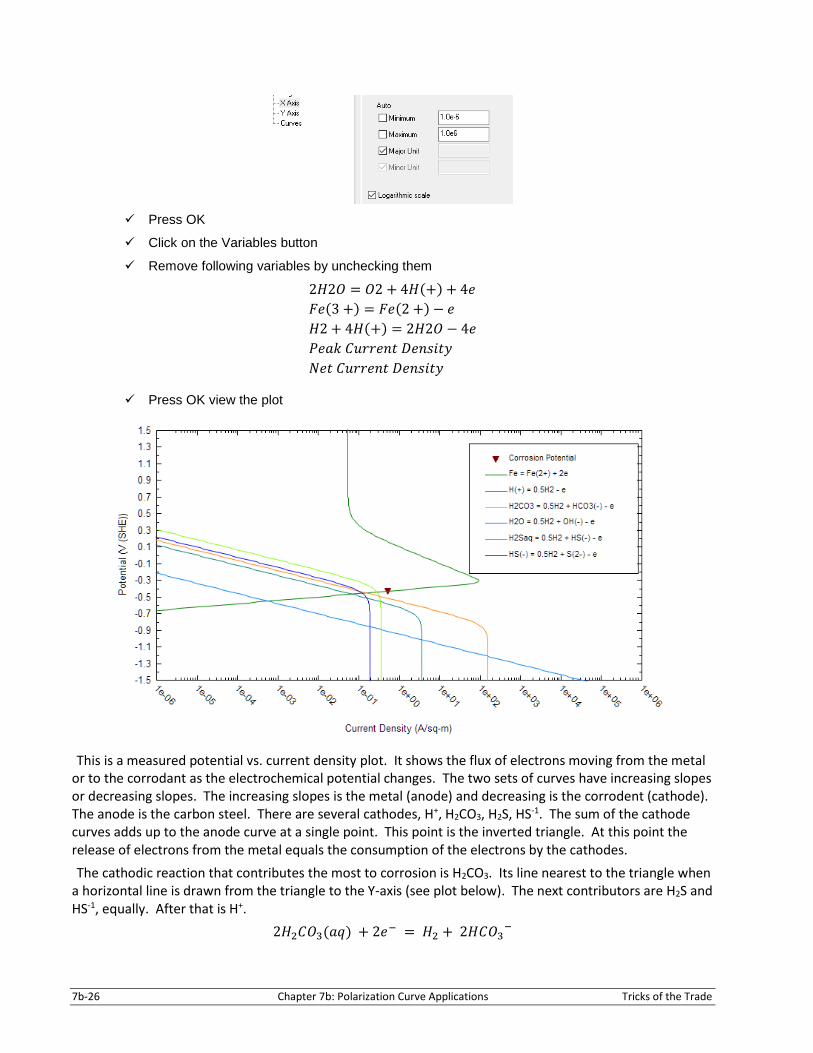
✓ Click on the Variables button
✓ Remove following variables by unchecking them
2𝐻2𝑂 = 𝑂2 + 4𝐻(+) + 4𝑒
𝐹𝑒(3 +) = 𝐹𝑒(2 +) − 𝑒
𝐻2 + 4𝐻(+) = 2𝐻2𝑂 − 4𝑒
𝑃𝑒𝑎𝑘 𝐶𝑢𝑟𝑟𝑒𝑛𝑡 𝐷𝑒𝑛𝑠𝑖𝑡𝑦
𝑁𝑒𝑡 𝐶𝑢𝑟𝑟𝑒𝑛𝑡 𝐷𝑒𝑛𝑠𝑖𝑡𝑦
✓ Press OK view the plot
This is a measured potential vs. current density plot. It shows the flux of electrons moving from the metal or to the corrodant as the electrochemical potential changes. The two sets of curves have increasing slopes or decreasing slopes. The increasing slopes is the metal (anode) and decreasing is the corrodent (cathode). The anode is the carbon steel. There are several cathodes, H+, H2CO3, H2S, HS-1. The sum of the cathode curves adds up to the anode curve at a single point. This point is the inverted triangle. At this point the release of electrons from the metal equals the consumption of the electrons by the cathodes.
The cathodic reaction that contributes the most to corrosion is H2CO3. Its line nearest to the triangle when a horizontal line is drawn from the triangle to the Y-axis (see plot below). The next contributors are H2S and HS-1, equally. After that is H+.
2𝐻2𝐶𝑂3(𝑎𝑞) + 2𝑒− = 𝐻2 + 2𝐻𝐶𝑂3−
Tricks of the Trade Chapter 7b: Polarization Curve Applications 7b-27
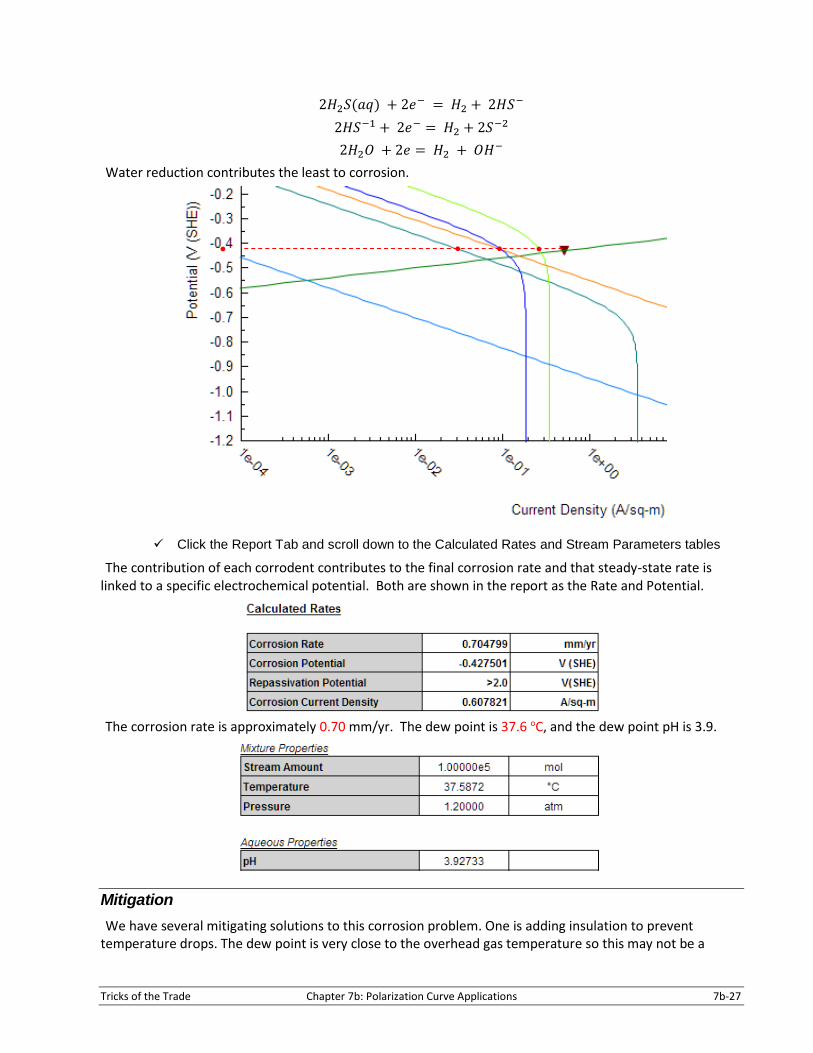
2𝐻2𝑆(𝑎𝑞) + 2𝑒− = 𝐻2 + 2𝐻𝑆−
2𝐻𝑆−1 + 2𝑒− = 𝐻2 + 2𝑆−2
2𝐻2𝑂 + 2𝑒 = 𝐻2 + 𝑂𝐻−
Water reduction contributes the least to corrosion.
✓ Click the Report Tab and scroll down to the Calculated Rates and Stream Parameters tables
The contribution of each corrodent contributes to the final corrosion rate and that steady-state rate is linked to a specific electrochemical potential. Both are shown in the report as the Rate and Potential.
The corrosion rate is approximately 0.70 mm/yr. The dew point is 37.6 oC, and the dew point pH is 3.9.
Mitigation
We have several mitigating solutions to this corrosion problem. One is adding insulation to prevent temperature drops. The dew point is very close to the overhead gas temperature so this may not be a

7b-28 Chapter 7b: Polarization Curve Applications Tricks of the Trade
suitable option. Adding heat to keep the temperature above the dew point is usually considered along with insulation. Changing the chemistry to change the partial oxidation and reduction processes is also an option. Furthermore, changing alloys could mitigate the corrosion problem.
Adjusting the solution chemistry
The condensate pH is approximately 3.9. We can try to add a base to increase the pH. In this section, we will add Diethanolamine to raise the pH to 7.5.
✓ Click on the Gas Condensate stream
✓ Add a Single Point calculation then rename it DEA
✓ Type DEA in the first available inflow cell
or
✓ Select Set pH from the Type of calculation
✓ Enter 7.5 or pH
✓ Click on the dropdown arrow for the pH Base Titrant and select DEA (or the corresponding name that appears: N,N-Diethanolamine or HN(C2H4OH)2.
The program is now set up to adjust the amount of DEA to match a target value of pH = 7.5.
✓ Calculate
✓ Review the Summary box
Tricks of the Trade Chapter 7b: Polarization Curve Applications 7b-29
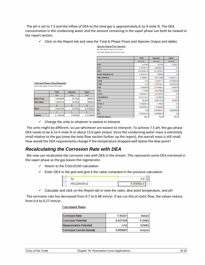
The pH is set to 7.5 and the inflow of DEA to the total gas is approximately 6.1e-4 mole %. The DEA concentration in the condensing water and the amount remaining in the vapor phase can both be viewed in the report section.
✓ Click on the Report tab and view the Total & Phase Flows and Species Output and tables
✓ Change the units to whatever is easiest to interpret
The units might be different, so use whichever are easiest to interpret. To achieve 7.5 pH, the gas-phase DEA needs to be 6.1e-4 mole % or about 15.6 ppm (mass). Since the condensing water mass is extremely small relative to the gas (view the total flow section further up the report), the overall mass is still small. How would the DEA requirements change if the temperature dropped well below the dew point?
Recalculating the Corrosion Rate with DEA
We now can recalculate the corrosion rate with DEA in the stream. This represents some DEA entrained in the vapor phase as the gas leaves the regenerator.
✓ Return to the CSG10100 calculation
✓ Enter DEA to the grid and give it the value computed in the previous calculation.
✓ Calculate and click on the Report tab to view the rates, dew point temperature, and pH
The corrosion rate has decreased from 0.7 to 0.48 mm/yr. If we run this at static flow, the values reduce from 0.4 to 0.27 mm/yr.

7b-30 Chapter 7b: Polarization Curve Applications Tricks of the Trade
The pH is 7.6, similar to the target value of 7.5. Therefore, neutralizing the pH had a partial effect on corrosion reduction.
Alloys
Since treating the acid gas with a base is probably not a good idea for metal hydroxides, perhaps we can change the alloy. We will add a new corrosion rates calculation and test different alloys.
✓ Copy the CSG10100 calculation back into the stream
o Right-mouse-click on the CSG10100 object and select Copy.
o Right-mouse-click on the Gas Condensate stream and select Paste
✓ Rename it ‘13% Cr’
✓ In the Contact Surface grid, Select 13%Cr stainless steel
✓ Change the flow conditions from Static to Pipe Flow, keeping the other default values
✓ Calculate
✓ Click on the Report and view the corrosion rates
The corrosion rates are an order of magnitude lower at ~60 um/yr. This is consistent with the use of 13% Cr to protect against CO2 corrosion.

Tricks of the Trade Chapter 7b: Polarization Curve Applications 7b-31
✓ Select the Polarization Curve tab
The curve has changed in two ways, first the 13%Cr curve has shifted upwards. It is 0.51 V instead of 0.67 V (a smaller relative driving force to oxidize). Second, because of the anode curve being shifted upwards, the intersection between the anode and cathode reaction (mixed potential) shifted to the left (lower current density).
The next step is to repeat with Stainless Steel 304.
✓ Copy the CSG10100 calculation again to create a new corrosion calculation
✓ Name it ‘SS304’
✓ Calculate
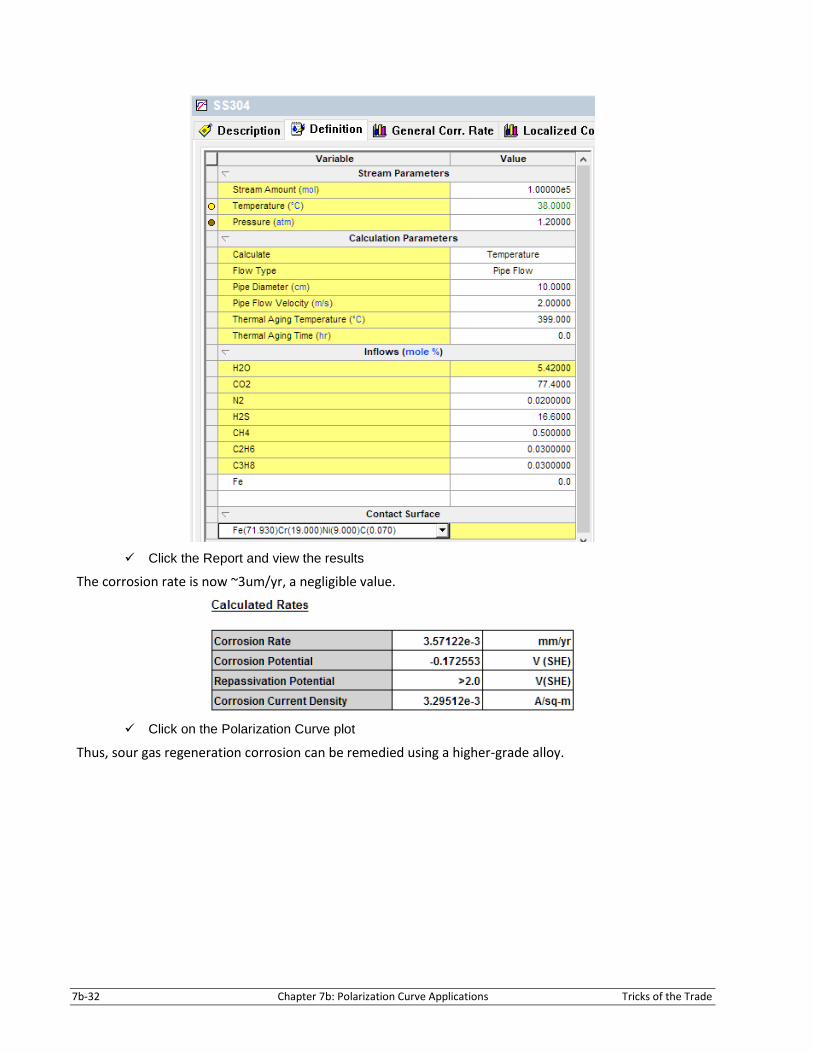
7b-32 Chapter 7b: Polarization Curve Applications Tricks of the Trade
✓ Click the Report and view the results
The corrosion rate is now ~3um/yr, a negligible value.
✓ Click on the Polarization Curve plot
Thus, sour gas regeneration corrosion can be remedied using a higher-grade alloy.

Tricks of the Trade Chapter 7b: Polarization Curve Applications 7b-33
Follow-up example
The effect of double-layer thickness on corrosion rates is evident from the previous case. The sudden change in slopes of the cathodes from slight negative to vertical is the result of the inability of those species to reach the surface at a high enough rate to accept the electrons that the surface is willing to provide it. If we consider the terms associated with diffusion to and from the surface, we can estimate these diffusion properties.
First, we know the maximum rate, or more specifically, flux at which each species is transported to the surface. It is the value in A/m2 on the polarization where the vertical line crosses. Using the last plot we
created (304SS), the values are 𝐶𝑂2 − 0.35𝐴
𝑚2 , 𝐻 + − 4.14
𝐴
𝑚2𝑎 and 𝐻2𝑆 – 190
𝐴
𝑚2
✓ Return to the report and find the concentration for these species
Your results may differ: 𝐶𝑂2 – 1011𝑝𝑝𝑚 (16.3𝑚𝑚𝑜𝑙𝑒
𝑘𝑔𝑠𝑜𝑙𝑢𝑡𝑖𝑜𝑛), 𝐻 + − 0.12𝑝𝑝𝑚 (0.12
𝑚𝑚𝑜𝑙
𝑘𝑔𝑠𝑜𝑙𝑢𝑡𝑖𝑜𝑛)
and 𝐻2𝑆 – 521.2𝑝𝑝𝑚 (15.33𝑚𝑚𝑜𝑙
𝑘𝑔𝑠𝑜𝑙𝑢𝑡𝑖𝑜𝑛).
The half reactions for the corrodants are 𝐶𝑂2 + 𝐻2𝑂 + 𝑒−= ½ 𝐻2 + 𝐻𝐶𝑂3−, 𝐻 + +𝑒− = ½ 𝐻2 and 𝐻2𝑆 +
𝑒−= ½ 𝐻2 + 𝐻𝑆, where e- in this case is one mole of electrons. Remembering, 𝐴 =𝐶
𝑠= 𝑒 −
𝑠 (𝐴 = 𝐴𝑚𝑝𝑒𝑟𝑒, 𝐶 = 𝐶𝑜𝑢𝑙𝑜𝑚𝑏), we can first calculate the maximum moles of each species that can reach
the surface each second. Since each species consumes a single mole of electrons in their reaction, then
resulting flux of species to the surface is 𝐶𝑂2 = 0.35𝑚𝑜𝑙𝑒𝑠
𝑠
𝑚2, 𝐻+ = 4.14
𝑚𝑜𝑙𝑒𝑠
𝑠
𝑚2 and 𝐻2𝑆 = 190
𝑚𝑜𝑙𝑒𝑠
𝑠
𝑚2.
If the system in question is a 1m3 cube filled with this solution, and if we assume a 1 g/cc density then the
total moles of each species becomes: 𝐶𝑂2 − 16.3𝑚𝑜𝑙𝑒𝑠
𝑚3𝑠𝑜𝑙𝑢𝑡𝑖𝑜𝑛, 𝐻 + − 0.12
𝑚𝑜𝑙𝑒𝑠
𝑚3𝑠𝑜𝑙𝑢𝑡𝑖𝑜𝑛 and 𝐻2𝑆 −
15.3𝑚𝑜𝑙𝑒𝑠
𝑚3𝑠𝑜𝑙𝑢𝑡𝑖𝑜𝑛.
Dividing the concentration by its maximum flux yields: 𝐶𝑂2 – 46.6𝑠
𝑚 0.0214
𝑚
𝑠, 𝐻 + − 0.029
𝑠
𝑚 34.5
𝑚
𝑠
and 𝐻2𝑆 – 0.805𝑠
𝑚 12.4
𝑚
𝑠. Pull the species mobilities from the report: 𝐶𝑂2 − 2.63𝑒 − 9
𝑚2
𝑠, 𝐻 +
− 1.13𝑒 − 8𝑚2
𝑠 and 𝐻2𝑆 − 2.45𝑒 − 9 𝑚.