Chapter 7 The Wave Equation in Fluids

Chapter 7The Wave Equation in Fluids

So far in this book, we dealt with vibrations. These are processes that vary as func-tions of time. We were able to describe relevant types of vibrations with commondifferential equations. The current chapter now focuses on waves. These are pro-cesses that vary with both time and space. Their mathematical description requirespartial differential equations.

Motivated by the electroacoustic analogies, we start with an excursion into elec-tromagneticwaves. The discussion brings us back to soundwaves in the next section.1

Figure7.1 illustrates the equivalent circuit for an elementary section of a homoge-neous, lossless electrical transmission line. For this section, the following loop andnode equations hold,

u −(u + ∂u

∂xdx

)= L ′ dx

∂i

∂t, and (7.1)

i −(i + ∂i

∂xdx

)= C ′ dx

∂u

∂t. (7.2)

The following two linear differential equations are obtained by neglecting the higher-order differentials, thus we get

− ∂u

∂x= L ′ ∂i

∂tand − ∂i

∂x= C ′ ∂u

∂t. (7.3)

This set of equations shows that a temporal variation of the slope of one of thevariables results in a proportional spatial variation of the slope of the other one. This

1 An advice for readers who have not yet heard of electromagnetic waves: Start with readingSects. 7.1–7.2.

© Springer-Verlag GmbH Germany, part of Springer Nature 2021N. Xiang and J. Blauert, Acoustics for Engineers,https://doi.org/10.1007/978-3-662-63342-7_7

97

REVISED P

ROOF

http://crossmark.crossref.org/dialog/?doi=10.1007/978-3-662-63342-7_7&domain=pdf

https://doi.org/10.1007/978-3-662-63342-7_7

98 7 The Wave Equation in Fluids

Fig. 7.1 Equivalent circuit for a differential section of a homogeneous, lossless electrical trans-mission line

causes the total energy on the line to swing between two types of complementaryenergies, namely,

– Magnetic energy per length, W ′ = 12 L

′ i2

– Electric energy per length, W ′ = 12C

′ u2

We now combine the two linear differential equations (7.3), to a differential equationof the second order, which is

∂2u

∂x2= 1

c2line, el

∂2u

∂t2. (7.4)

This is the so-called wave equation, here in the formulation for electromagneticwaves on an electrical transmission line. Hereby c line, el is the propagation speed ofelectromagnetic waves on the transmission line, namely,

c line, el = 1√L ′ C ′ . (7.5)

In acoustics, we also have waves that propagate along with one coordinate, forexample, in gas-filled tubeswith diameters that are small compared to thewavelength.Such longitudinal compression waves are schematically sketched in Fig. 7.2.

Fig. 7.2 One-dimensional longitudinal acoustic wave. Zones of compression and rarefaction areschematically indicated

REVISED P

ROOF

7 The Wave Equation in Fluids 99

Two complementary forms of energies are again required for these types of waves tooccur, but in this casewe choose energies per volume. In this way, we stay compatiblewith the use of p and v as characteristic sound-field quantities. We thus get,

– Potential energy per volume, W ′′ = 12κ p2 κ ...volume compressibility

– Kinetic energy per volume, W ′′ = 12� v2 � ...mass density

Mimicking the wave equation for the electromagnetic waves, we consequently sug-gest the following wave equations for one-dimensional acoustic waves,

− ∂ p

∂x= �

∂v

∂tand − ∂v

∂x= κ

∂ p

∂t, or − ∂v

∂x= 1

� c2∂ p

∂t, (7.6)

and the combined-second order expression as

∂2 p

∂x2= 1

c2∂2 p

∂t2, (7.7)

with the propagation speed of sound waves to be

c = 1√κ �

, (7.8)

and the volume compressibility to be

κ = 1

� c2. (7.9)

The relevant question is now whether these supposed equations, which are so neatlyanalog to electric expressions, are actually in compliance with the physical reality.The answer is yes, at least approximately. Yet, there are several features of the mediawhere sound exists that must be taken as idealized. A total of five linearizations isnecessary. The following section elaborate on these.

7.1 Derivation of the One-Dimensional Wave Equation

We assume an idealized medium as a model of the real physical medium. Onlycompression and expansion but no shear stress are allowed. This restriction limitsus to a media category called fluids. Many gases and liquids are treatable treatedas fluids. Fluids only experience longitudinal waves. The following features of theidealized medium are assumed.

– The medium is homogeneous and does not crack, meaning that there are noinclusions of vacuum as might be caused by cavitation.

– The thermal conductivity is zero. This assumes adiabatic compression.

REVISED P

ROOF


– The inner friction is zero, meaning that there are no energy losses and noviscosity.

– The medium has a defined mass and elasticity.

We now assume that themedium is not flowing and that there is no drift, meaning thatv− ≈ 0. The alternating part of the pressure be small compared to the static pressure,that is, p− � p∼. The alternating part of the density is also small in comparisonto the static one, in other words, �− � �∼. This results in a so-called small-signaloperation of the medium.

To arrive at the wave equation, we recollect three fundamental physical relation-ships. These are listed in the following.

• Hooke’s law, applied to fluids

• Newton’s mass law

• The mass-conservation law

We now formulate these three relationships in their differential forms as required forthe rest of our discussion. In differential form, they are known as

• State equation

• Euler’s equation

• Continuity equation

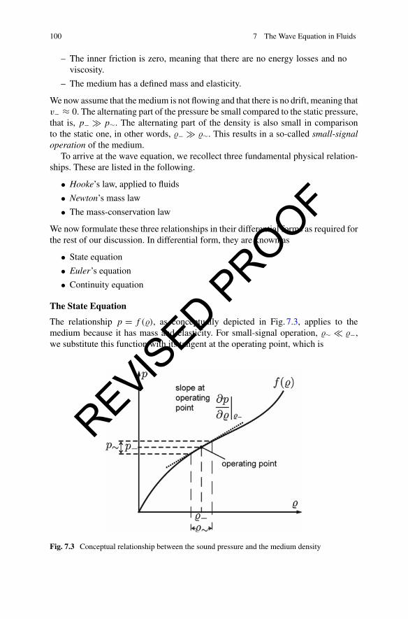
The State Equation

The relationship p = f (�), as conceptually depicted in Fig. 7.3, applies to themedium because it has mass and elasticity. For small-signal operation, �∼ � �−,we substitute this function with its tangent at the operating point, which is

Fig. 7.3 Conceptual relationship between the sound pressure and the medium density

REVISED P

ROOF

7.1 Derivation of the One-Dimensional Wave Equation 101

p∼ = ∂ p

∂�

∣∣∣�−

�∼ or p∼ = c2 �∼ . (7.10)

This leads us to the state equation in the form

∂� = 1

c2∂ p

∣∣∣�−

or c =√

∂ p

∂�

∣∣∣�−

. (7.11)

In this way, wemake our first linearization by assuming a linear spring characteristicfor the fluid.We prove later that c is the speed of sound,which is specific for amaterialbut depends on its temperature, humidity, and static pressure.

The proportionality coefficient in the state equation, c2, is estimated theoreticallyfor most single-atom gases by assuming a perfect gas. If such a gas is compressed inthe absence of heat conduction, we have so-called adiabatic compression. The thenapplicable adiabatic law of thermodynamics states that

p V η = const = p− V η− , (7.12)

where V is the volume of a mass element concerned, and η = cp/cv (usually knownas γ) is the ratio of the specific heat capacities,2 with which we derive

p =(V−V

)η

p− =(

�

�−

)η

p− . (7.13)

Differentiation of this expression at the position � = �− renders the following expres-sion,

∂ p

∂�

∣∣∣�−

= η

(�

�−

)η−1

︸︷︷︸1 for � = �−

1

�−p− , (7.14)

and then, consequently,∂ p

∂�

∣∣∣�−

= c2 = η p−�−

. (7.15)

Finally we get for the speed of sound in the perfect gas,

c =√

η p−�−

=√

1

�− κ−, (7.16)

2 These quantities are taken from thermodynamics, where cp is the specific heat capacity at constantpressure and cv the specific heat capacity at constant volume.

REVISED P

ROOF


Table 7.1 Values of typical materials

Material Density, �− Sound speed, c Characteristicimpedance, Zw

Air at 1000hPa and20 ◦C

1.2 kg/m3 343m/s 412Ns/m3

Water at 10 ◦C 1000 kg/m3 1440m/s 1.44 · 106 Ns/m3

Steel (longitudinalwave)

≈ 7500 kg/m3 ≈6000m/s ≈45 · 106 Ns/m3

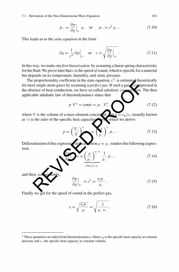
Fig. 7.4 An accelerated differential mass, dm, of fluid in a tube

where

κ− = κ |�−= 1/(η p−) = 1

�− c2. (7.17)

This expression is very similar to the one for liquids, but there the reciprocal value ofthe volume compressibility, or bulk compressibility, κ, the so-called the compressionmodulus, which is K = 1/κ, is more often used. Some specific material values aregiven in Table7.1.3

Euler’s Equation

Figure7.4 depicts a differential mass of gas in a tube with rigid walls and a diametersmall compared to the wavelength. The mass element is accelerated due to a pressuredifference. The total differential of the particle velocity, v, being a function of timeand space, is

dv (x, t) = ∂v

∂tdt + ∂v

∂xdx . (7.18)

From this we arrive at the acceleration, a,

a = dv

dt= ∂v

∂t+ ∂v

∂x

dx

dt, where

dx

dt= v . (7.19)

3 The characteristic field impedance, Zw, also known as wave impedance, is introduced in Sect. 7.4.

REVISED P

ROOF

7.1 Derivation of the One-Dimensional Wave Equation 103

Fig. 7.5 A spatially-fixed differential volume, dV , of fluid in a tube

According to Newton’s mass law, F = m · a, we now write

A

[p −

(p + ∂ p

∂xdx

)]= (� A dx)

(∂v

∂t+ ∂v

∂xv

), (7.20)

which is Euler’s equation.Note that a second linearization is implemented by the replacement of � with

its static value, �−. Further, the second term in the sum, v · (∂v/∂x), is usuallyirrelevant in acoustics since v is zero in resting media, and also because the variationof v over space is usually small. This means that this term is a differential of thesecond order. Neglecting it, constitutes our third linearization.4 We thus arrive at ourfirst linear wave equation as follows,

− ∂ p

∂x= �−

∂v

∂t. (7.21)

The Continuity Equation

Figure7.5 depicts a fixed volume in a tubewheremass flows in and out. This situationfollows themass-conservation law, which states that what flows in and does not comeout again remains inside the volume since mass does not vanish.

The mass flowing in during a time interval, dt , is

dm in = A �−

dx︷︸︸︷v dt , (7.22)

and the mass flowing out during the same time interval is

dm out = A �− v dt + A �−∂v

∂xdx dt . (7.23)

4 Consider whether this linearization is still justified when the medium is flowing fast as it does inan exhaust system, and/or if there are rapid changes of v over x as occur at area steps in a tube. Thesecond term is the more significant one in flow dynamics while the first term is typically neglectedin that scientific field.

REVISED P

ROOF


The difference, also known as the mass surplus, is

dm� = −A �−∂v

∂xdx dt . (7.24)

If the mass inside the volume has changed, the mass density in the volume must havealso changed, allowing us to write the mass surplus as

dm� = A dx∂�

∂tdt . (7.25)

Combining the two surplus expressions yields

− �−∂v

∂x= ∂�

∂t, (7.26)

which is the continuity equation.

Since we want to use the field quantities p and v, we now substitute p by v byapplying the state equation (7.11) as follows,

∂�− = ∂ p

c2= κ−�− ∂ p . (7.27)

Combining equations (7.26) and (7.27), finally renders the second linear differentialwave equation as

− ∂v

∂x= κ−

∂ p

∂t, (7.28)

with κ− = 1/(�− c2). Note that κ has been replaced by κ−, which is our fourthlinearization.5

7.2 Three-Dimensional Wave Equation in CartesianCoordinates

The two wave equations that we just derived are valid for a one-dimensional axialwave in a tube. The walls of the tube do not play any role since we have a purelylongitudinal wave that propagates parallel to the walls.

5 Because of κ− ≈ κ and �− ≈ �, we omit the subscripts of κ− and �− from now on to simplifythe notation—such as in κ = 1/(� c2).

REVISED P

ROOF

7.2 Three-Dimensional Wave Equation in Cartesian Coordinates 105

Fig. 7.6 Bundle of tubes with one-dimensional waves in them

Our equations are also valid for a bundle of tubes—shown inFig. 7.6—andnothingwould change concerning the wave if we took the tubes away. Consequently, theequations still hold for one-dimensional longitudinal waves in infinitely extendedmedia.

As there is no shear stress in fluids, waves from different orthogonal directions inthe medium just superimpose without influencing each other. This property allowsus to formulate the three-dimensional wave equations in Cartesian coordinates bysuperimposing the wave components of the x−, y−, and z−direction. Denoting −→x ,−→y , and −→z for the unit vector along the x − −, y − −, and z − −directions, weutilize the three operators taken from vector analysis,

Gradient

−−−→grad p = −→∇ p =

{∂ px∂x

; ∂ py∂y

; ∂ pz∂z

}

={∂ px

∂x−→x + ∂ py

∂y−→y + ∂ pz

∂z−→z

}. . . a vector (7.29)

Divergence

div · −→v = ∇ · −→v ={∂vx

∂x+ ∂vy

∂y+ ∂vz

∂z

}, . . . a scalar (7.30)

Laplacian

div · −−−→grad p = ∇2 p =

{∂2 px∂x2

+ ∂2 py∂y2

+ ∂2 pz∂z2

}, . . . a scalar (7.31)

REVISED P

ROOF


Using these operators, we write the following handsome set of linear acoustical waveequations for lossless fluids, with v and p denoting first-order time derivatives,

− grad p = � v , (7.32)

and

− div · v = κ p = 1

� c2p , (7.33)

where we have omitted the vector arrows for simplicity. Combination of (7.32) and(7.33) renders the wave equation with the second-order time derivative,

∇2 p = 1

c2p . (7.34)

The corresponding equations for the particle velocity, v, shown below, looks formallyidentical,6 namely,

∇2v = 1

c2v . (7.35)

Note that both the first-order (7.32)–(7.33) and the second-order wave equations(7.34)–(7.35) are of general form and independent of the actual coordinate systems.

7.3 Solutions of the Wave Equation

We now present some prominent solutions of the wave equation. To keep the dis-cussion simple, we restrict ourselves to one-dimensional cases, specifically the waveequation in its following the formulation,7 as predicted at the beginning of thischapter.

∂2 p

∂x2= 1

c2∂2 p

∂t2. (7.36)

Two or three-dimensional solutions evolve from superposition of one-dimensionalsolutions.

General Solution

The following general solution is known as the d’Alembert solution. d’Alembertassumes two waves propagating in opposite directions, x and −x . Both the forward-progressing and returning waves have the same speed, c. The solution is writtenas

6 In theoretical acoustics, the velocity potential, fl, is frequently used. It is defined as−→v = −−−−−→gradΦ.

Its wave equation is ∇2 Φ = (1/c2) Φ.7 This form follows also from combining the differential of x in (7.21) with that of t in (7.28).

REVISED P

ROOF

7.3 Solutions of the Wave Equation 107

p(x, t) = p→(t − x

c

)+ p←

(t + x

c

). (7.37)

Note that, since this equation is a differential equation of the second order, it issatisfied by any function f (t ± x/c) that is differentiable twice with respect to bothtime and space. In the above equation, p→( · ) and p←( · ) denote two functions withopposite directions of propagation along the x-axis.

Solution for Harmonic Functions

This solution, called the Bernoulli solution, is a special case of d’Alembert’s solutionapplied to harmonic functions (sinusoids). Dealing with harmonic functions allowsus to take advantage of complex notation by rewriting the wave equation as follows,

∂2 p

∂x2− (jβ)2 p = 0 . (7.38)

This is known as the Helmholtz form, in which

β = ω

c= ω

√� κ , (7.39)

is called phase coefficient.8

The solution unfolds from trying p = e γ x . This approach leads to the character-

istic equation, γ2 = (jβ)2, and its solutions,9 γ1, 2

= ±(jβ). These solutions againallow for two waves in opposite directions, namely,

p(x) = p→e −jβ x + p←e +jβ x . (7.40)

Similarly, the solutions for the particle velocity is expressible as

v(x) = v →e −jβ x + v ←e +jβ x . (7.41)

Both the forward progressing and the returning waves go through a complete periodfor β λ = 2π, with λ being the wavelength, we obtain the well-known formulas

λ f = c and β = ω

c= 2π

λ. (7.42)

8 In physics this quantity is often called wave number or, more precisely, angular wave number anddenoted by k. In fact, it is not a “number" as it has the dimension [1/length].9 γ is called complex propagation coefficient, also denoted complex wave number, k. We make useof it later, particularly, in Sects. 8.3 and11.2.

REVISED P

ROOF


7.4 Field Impedance and Power Transport in Plane Waves

First we look at the forward progressing wave, expressed as

p(x) = p→e−jβ x and v(x) = v →e−jβ x . (7.43)

Following Euler’s equation (7.21), we obtain

�∂v

∂t= −∂ p

∂xand jω v → e−jβ x � = −(−jβ) p→ e−jβ x (7.44)

and, finally, considering the returning way likewise,

Zw = p→ e−jβ x

v →e−jβ x= − p← e+jβ x

v ← e+jβ x= � c =

√�

κ. (7.45)

The real quantity, Zw, is known as characteristic field impedance or waveimpedance.10 Since Zw is real in our case, sound pressure and particle velocity arein phase, which generally holds for plane waves in lossless fluids.

The thus purely resistive (active) intensity, I = Re{ I }, transported by the forwardprogressing wave is

I = 1

2Re

[p→e−jβ x

(v → e−jβ x

)∗] = 1

2|p→| |v →| = 1

2Zw| v →|2 , (7.46)

which also holds for the returning wave. The transported active power, P , resultsfrom multiplying the intensity with the area which it crosses perpendicularly. Thismultiplication resulting in the following scalar product of two vectors, P = −→

I · −→A⊥.

7.5 Transmission-Line Equations and Reflectance

As previously mentioned, there is only axial wave propagation in tubes with muchsmaller diameters than the wavelengths, d � λ.

Since the ratio of p and v inside the tube is only dependent on the terminatingimpedance of the tube, Z 0 = p

0/v 0, it is convenient to formulate the solution of

the wave equation in terms of the distance from the position of Z 0. To this end, wesubstitute the coordinate x with −l as shown in Fig. 7.7.

10 When considering losses in themedium, Z w becomes complex due to the addition of an imaginarycomponent.

REVISED P

ROOF

7.5 Transmission-Line Equations and Reflectance 109

Fig. 7.7 One dimensional wave in a tube with a termination

Now, because of e ±jβ l |l=0 = 1 at position l = 0, we have p0

= p→ + p←and v 0 = v → + v ← . Keeping (7.45) in mind, we further have Zw = p→/v → =−p←/v ←, which leads to the expressions

Zw v 0 = p→ − p← and p0/Zw = v → − v ← . (7.47)

Consequently it follows that

p→ = 1

2

(p0+ Zw v 0

)p← = 1

2

(p0− Zw v 0

)(7.48)

v → = 1

2

( p0

Zw+ v 0

)v ← = −1

2

( p0

Zw− v 0

). (7.49)

For an arbitrary position, l = −x , the following expressions result,

p(l) = 1

2

(p0+ Zw v 0

)e jβ l + 1

2

(p0− Zw v 0

)e −jβ l and (7.50)

v(l) = 1

2

( p0

Zw+ v 0

)e jβ l − 1

2

( p0

Zw− v 0

)e−jβ l . (7.51)

Complex decompositionwith e−jα = cosα − j sinα leads to the following two equa-tions that are known as transmission-line equations,11 namely,

p(l) = p0cos(β l) + jZw v 0 sin(β l) , (7.52)

v(l) = jp0

Zwsin(β l) + v 0 cos(β l) , (7.53)

or in matrix form

11 This name originates from electrical engineering where the same equations hold but with p beingreplaced by u and v by i .

REVISED P

ROOF


[p(l)v(l)

]=

[cos(βl) jZw sin(βl)

j sin(βl)/Zw cos(βl)

] [p0

v 0

]. (7.54)

Another popular way of writing these equations is

p(l)

p0

= cos(βl) + jZw

Z 0sin(βl) , (7.55)

v(l)

v 0= cos(βl) + j

Z 0

Zwsin(βl) . (7.56)

We now discuss different terminations of the tube. The following three cases areof particular interesting in this context.

(1) Z 0 = p0/v 0 = Zw This means that there is no reflection at the terminal,

and all power moves on. This case is called wave match and results in noreturning wave. Consequently, (7.52) becomes

p(l) = p0e jβ l . (7.57)

(2) Z 0 = ∞ and, hence, v 0 = 0 This case is called hard termination and isachieved by closing the tube with a rigid surface. In this case, the forwardprogressing wave is fully reflected, and zero power leaves through theterminal. Equations (7.52) and (7.53) render

p(l) = p0cos(βl) and v(l) = j

p0

Zwsin(βl) . (7.58)

These two formulas describe a so-called standing wave. The sound pres-sure varies at all positions sinusoidally as a function of time. Sound pres-sure and particle velocity are 90◦ out of phase.

(3) Z 0 = 0 and, thus, p0

= 0 Now the end of the tube is open, resulting insoft termination

p(l) = jZw v 0 sin(βl) and v(l) = v 0 cos(βl) (7.59)

Neglecting any radiationout of the open end—which is of course idealizing—the sound pressure is zero on the terminating plane. The forward progress-ing and the returning wave superimpose again to a standing wave, but theyhave a different phase angle than the one in the hard-termination case.Again, there is no power leaving through the terminal.

The reflectance, R, is a useful quantity for describing the reflection at the terminalplane of the tube. Using (7.48), it is defined as

R = p←p→

= ( p0− Zw v 0 )/2

( p0+ Zw v 0 )/2

= Z 0 − Zw

Z 0 + Zw. (7.60)

REVISED P

ROOF

7.5 Transmission-Line Equations and Reflectance 111

We have R = 0 for wave match, R = +1 for hard/rigid termination and R = −1for soft termination. If intensity or power are under consideration, the followingdefinitions12 are often used.

|R|2 …Degree of reflection

1 − |R|2 …Degree of absorption, α.

7.6 The Acoustic Measuring Tube

The acoustic measuring tube, also known as Kundt’s tube, is applied to measurefield impedances and reflectances in the terminal plane of a tube. Such a tube isschematically shown in Fig. 7.8. The tube is excited by a sound source from oneend—a sinusoidal sound in our case. The other end is terminated by the impedanceto be measured. There is an arrangement of absorbing material in front of the sourceto avoid back reflection.

Classical Method

A microphone moves along the axis of the tube and measures the sound pressure asa function of its position. The sound pressure inside the tube follows the followingequation, whereby R = |R| e jφR ,

p (l) = p→ (e+jβ l + R e−jβ l) = p→[e+jβ l + | R |e−j(β l−φR)

]. (7.61)

For any | R | �= 0, this function shows maxima and minima along l. In other words,a standing-wave behavior shows up—depicted in the lower panel of Fig. 7.8. Themaxima are located at all positions of l where the phase angles of the two terms in(7.61) are equal, the minima accordingly, where the phase angles are opposite. Thepositions of the extremes thus are,

β l = −(β l − φR) ± nπ, (7.62)

with minima when n is odd, and maxima when n is even.This results in the following standing-wave ratio, S,

S =∣∣∣∣ pmax

pmin

∣∣∣∣ = 1 + | R |1 − | R | , (7.63)

12 In the literature, these terms are often called reflection coefficient and absorption coefficient.However, their dimension is [1] and their value range is 0–1, or 0%–100%, respectively. This iswhy we prefer the term degree here .

REVISED P

ROOF


Fig. 7.8 Kundt’s tube for impedance measurement

from which we obtain the magnitude of the reflectance13 as

| R |(l = 0) = S − 1

S + 1. (7.64)

The phase angle of the reflectance, φR, is given by the position of the first minimum,lmin. It results from

φR(l = 0) = β lmin . (7.65)

Transfer-Function Method

In an alternative approach, the so-called transfer-function method, the complexreflectance, R (l = 0), and, consequently, the terminating impedance, Z 0 = p

0/v 0,

is measured without a microphone to be shifted mechanically. Instead, two micro-phones at a mutual distance of l� = l2 − l1 are employed at the positions2and1—depicted in Fig. 7.9. Starting from (7.52), we write14

p2

= p1cos(β l�) + jZw v 1 sin(β l�) and, thus, (7.66)

p2

p1

= cos(β l�) + jZw

Z 1sin(β l�), or (7.67)

13 The theory ofKundt’s tube is homomorphic to the theory of themeasuring line for electromagneticwaves. To convert reflectance into impedance, and vice versa, a graphical tool called Smith chartis useful. It transforms the plot of a function in the complex Z -plane into the corresponding plot inthe complex R-plane.14 Note that all involved distances, that is, l1, l2 and l� = l2 − l1, have positive values.

REVISED P

ROOF

7.6 The Acoustic Measuring Tube 113

Fig. 7.9 Impedance measurement with the transfer-function method

Z 1 = jZw sin(β l�)

( p2/p

1) − cos(β l�)

. (7.68)

With a straight-forward transformation along the distance −l2, which follows fromthe transmission-line equations (7.55) and (7.56), Z 2 transformes into the impedanceat the surface of the probe to be tested, Z0. The relevant formula is

Z 0 = Z 1 cos(βl1) + jZw sin(βl1)

cos(βl1) + j(Z 1/Zw) sin(βl1), (7.69)

In a similar way, we obtain a widely used formula for the complex reflectance,namely

R = ( p1/p

2) − e−jβ l�

e+jβ l� − ( p1/p

2)e+j2β l2 . (7.70)

The ratio of p1/p

2= T pp for a given frequency,ω1, is a transfer factor. Its frequency

function, H pp(ω), is called a transfer function. This fact lends the method its name.The transfer-functionmethod fails for frequencies where the nominator or denom-

inator in (7.69) or (7.70) is equal to zero. This is the case whenever l� = λ/2. Tocover awide frequency range, the condition l� < π c/ωmust be fulfilled. To this end,more than twomicrophones at different positions are employed—or one microphonethat measures sequentially at different positions.

7.7 Exercises

Wave Equation in Fluids, Solutions, Kundt’s Tube

Problem 7.1 An impulsive disturbance in a fluid medium propagates along a thintube as illustrated in Fig. 7.10. The wavelength is much longer than the tube diameter.To ease the solution, the sawtooth-formed impulses can be simplified by straightdotted lines.

REVISED P

ROOF


Fig. 7.10 A form-of-sawtooth impulse, propagating along a narrow tube

(a) The sawtooth-formed pressure impulse propagates along a tube—seeFig. 7.10. Sketch the reflected pressure impulse, and the superpositionbetween the forward-propagating and reflected pressure impulses withthe tube being rigidly terminated. Sketch at least more than four refinedsteps as indicated in Fig. 7.10.

(b) Consider now that a sawtooth-formed velocity impulse propagates alonga tube. Sketch the reflected velocity impulse and the superposition of theforward-propagating and reflected impulses with the tube being rigidlyterminated. Sketch at least more than four refined steps as indicated inFig. 7.10.

Problem 7.2 A thin tube—with a diameter of d � λ, that is, much smaller than thewavelength—is terminated by an impedance, Z 0, see Fig. 7.7. p

0and v 0 are the

sound pressure and the velocity at the termination.

Prove that the following holds,

Zw v 0 = p→ − p← and p0/Zw = v → − v ← (7.71)

p→ = 1

2

(p0+ Zw v 0

)and p← = 1

2

(p0− Zw v 0

)(7.72)

v → = 1

2

( p0

Zw+ v 0

)and v ← = −1

2

( p0

Zw− v 0

), (7.73)

as stated in (7.47), (7.48), and (7.49) .

Problem 7.3 A thin tube with a length, L , and a wave resistance, ZL, is terminatedby an impedance, Z0. At location L , which is the input port to the tube, a plane waveenters the tube and travels toward its termination, ZL.

(a) Determine, in general form, the input impedance of the tube.

(b) Consider the special cases of Z0 = 0, Z0 = ∞, and Z0 = ZL. How is thesound pressure distributed in these particular cases?

Problem 7.4 Similar to the sound pressure inside the tube in (7.57) with a termi-nation expressed by a reflectance, R = | R | e jφr , and the complex sound pressureexpressed as (7.61),

p (l) = p→[e+jβ l + | R | e−j(β l−φR)

](7.74)

REVISED P

ROOF

7.7 Exercises 115

(a) Calculate the magnitude (envelope) of p (l), that is, | p(l)|, of the complexsound pressure.

(b) Express the conditions for the envelope, | p(l)|, to assume minima (nodes)or the maxima (anti-nodes).

(c) Determine the ratio of the maxima and the minima of the sound-pressureenvelope.

(d) Derive the relations of the locations of the standing-wave nodes and anti-nodes and the termination impedance.

Problem 7.5 Derive the wave equation of an oscillating string under the small-displacement assumption, in other words, that displacements induced by the stringoscillations are much smaller than the length of the string.

REVISED P

ROOF

Chapter 7 The Wave Equation in Fluids

Documents

Transcript of Chapter 7 The Wave Equation in Fluids