Chapter 7Optimization Methods

IntroductionIntroduction• Examples of optimization problems

IC d i ( l t i i )– IC design (placement, wiring)– Graph theoretic problems (partitioning, coloring, vertex

covering)g)– Planning– Scheduling– Other combinatorial optimization problems (knapsack, TSP)

• Approaches A h– AI: state space search

– NN– Genetic algorithms– Genetic algorithms– Mathematical programming

IntroductionIntroduction

• NN models to coverNN models to cover– Continuous Hopfield mode

• Combinatorial optimizationCombinatorial optimization– Simulated annealing

• Escape from local minimumEscape from local minimum– Boltzmann machine (§6.4) – Evolutionary computing (genetic algorithms)Evolutionary computing (genetic algorithms)

Introduction• Formulating optimization problems in NN

– System state: S(t) = (x1(t) x (t)) where xi(t) is the currentSystem state: S(t) (x1(t), …, xn(t)) where xi(t) is the current value of node i at time/step t

• State space: the set of all possible states– State changes as any node changes its value based on

• Inputs from other nodes; Inter-node weights; Node functioni f ibl if i i fi ll i i h f h– A state is feasible if it satisfies all constraints without further

modification (e.g., a legal tour in TSP)A solution state is a feasible state that optimizes some given– A solution state is a feasible state that optimizes some given objective function (e.g., a legal tour with minimum length)

• Global optimum: the best in the entire state space• Local optimum: the best in a subspace of the state space (e.g., cannot be better by changing value of any SINGLE node)

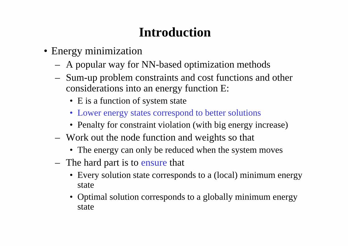
Introduction• Energy minimization

– A popular way for NN-based optimization methodsA popular way for NN based optimization methods– Sum-up problem constraints and cost functions and other

considerations into an energy function E:• E is a function of system state• Lower energy states correspond to better solutions

P lt f t i t i l ti ( ith bi i )• Penalty for constraint violation (with big energy increase)– Work out the node function and weights so that

• The energy can only be reduced when the system movesThe energy can only be reduced when the system moves– The hard part is to ensure that

• Every solution state corresponds to a (local) minimum energy y p ( ) gystate

• Optimal solution corresponds to a globally minimum energy statestate

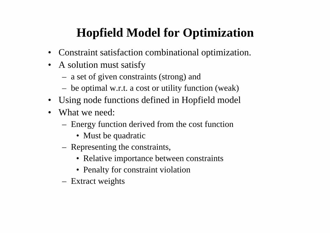
Hopfield Model for Optimizationp p• Constraint satisfaction combinational optimization.• A solution must satisfy• A solution must satisfy

– a set of given constraints (strong) and – be optimal w.r.t. a cost or utility function (weak)be optimal w.r.t. a cost or utility function (weak)

• Using node functions defined in Hopfield model• What we need:

– Energy function derived from the cost function• Must be quadratic

– Representing the constraints, • Relative importance between constraints• Penalty for constraint violation• Penalty for constraint violation

– Extract weights

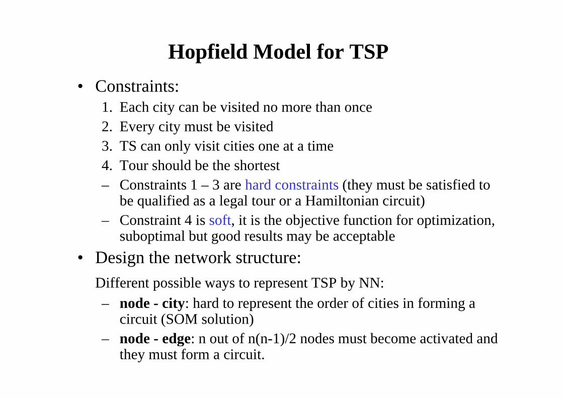
Hopfield Model for TSP• Constraints:

1 Each city can be visited no more than once1. Each city can be visited no more than once2. Every city must be visited3. TS can only visit cities one at a time4. Tour should be the shortest– Constraints 1 – 3 are hard constraints (they must be satisfied to

be qualified as a legal tour or a Hamiltonian circuit)be qualified as a legal tour or a Hamiltonian circuit)– Constraint 4 is soft, it is the objective function for optimization,

suboptimal but good results may be acceptable• Design the network structure:

Different possible ways to represent TSP by NN:p y p y– node - city: hard to represent the order of cities in forming a

circuit (SOM solution)d d t f ( 1)/2 d t b ti t d d– node - edge: n out of n(n-1)/2 nodes must become activated and

they must form a circuit.

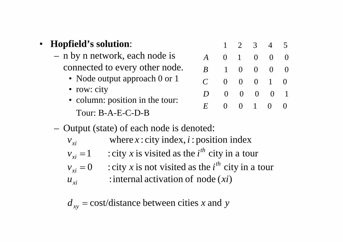
• Hopfield’s solution:– n by n network, each node is

connected to every other node0001054321

Aconnected to every other node.

• Node output approach 0 or 1• row: city 10000

0100000001

DCB

y• column: position in the tour:

Tour: B-A-E-C-D-B0010010000

ED

– Output (state) of each node is denoted:ixv

thxi indexposition: index,city:where

iixv

ixvth

xi

thxi

)(dfi ii ltouraincitytheasvisitednotiscity:0

touraincitytheasvisitediscity:1

yxd

xiuxi

andcitiesbetweenncecost/dista

)(node ofactivationinternal:

yxdxy andcitiesbetweenncecost/dista

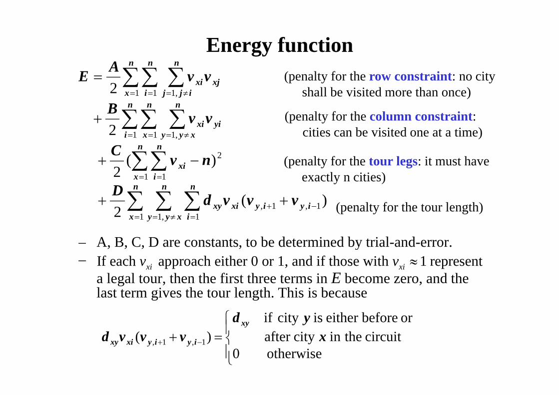
Energy functionn n nA

n n n

n

x

n

i

n

ijjxjxi

B

vvAE1 1 ,1

2

(penalty for the row constraint: no city shall be visited more than once)

n ni x xyy

yixi

C

vvB

2

1 1 ,12 (penalty for the column constraint:

cities can be visited one at a time)

n n nx i

xi

dD

nvC1 1

2

)(

)(2

(penalty for the tour legs: it must have exactly n cities)

A B C D are constants to be determined by trial and error

x xyy i

iyiyxixy vvvd1 ,1 1

1,1, )(2 (penalty for the tour length)

– A, B, C, D are constants, to be determined by trial-and-error.–

a legal tour, then the first three terms in E become zero, and the If each approach either 0 or 1, and if those with 1 representxi xiv v

last term gives the tour length. This is because

i ihiiforbeforeeitheriscityif

)(yd

dxy

otherwise 0circuittheincityafter)( 1,1, xvvvd iyiyxixy

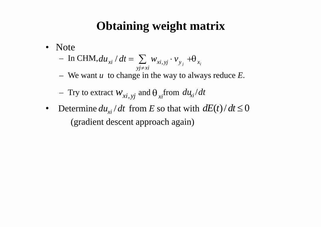
Obtaining weight matrix

• Note– In CHM, xyyjxixi vwdtdu /,

– We want u to change in the way to always reduce E. ij x

xiyjyyjxixi

,

– Try to extract and from

• Determine from E so that with yjxiw , dtduxi /

dtduxi / ( ) / 0dE t dt xi

(gradient descent approach again)xi

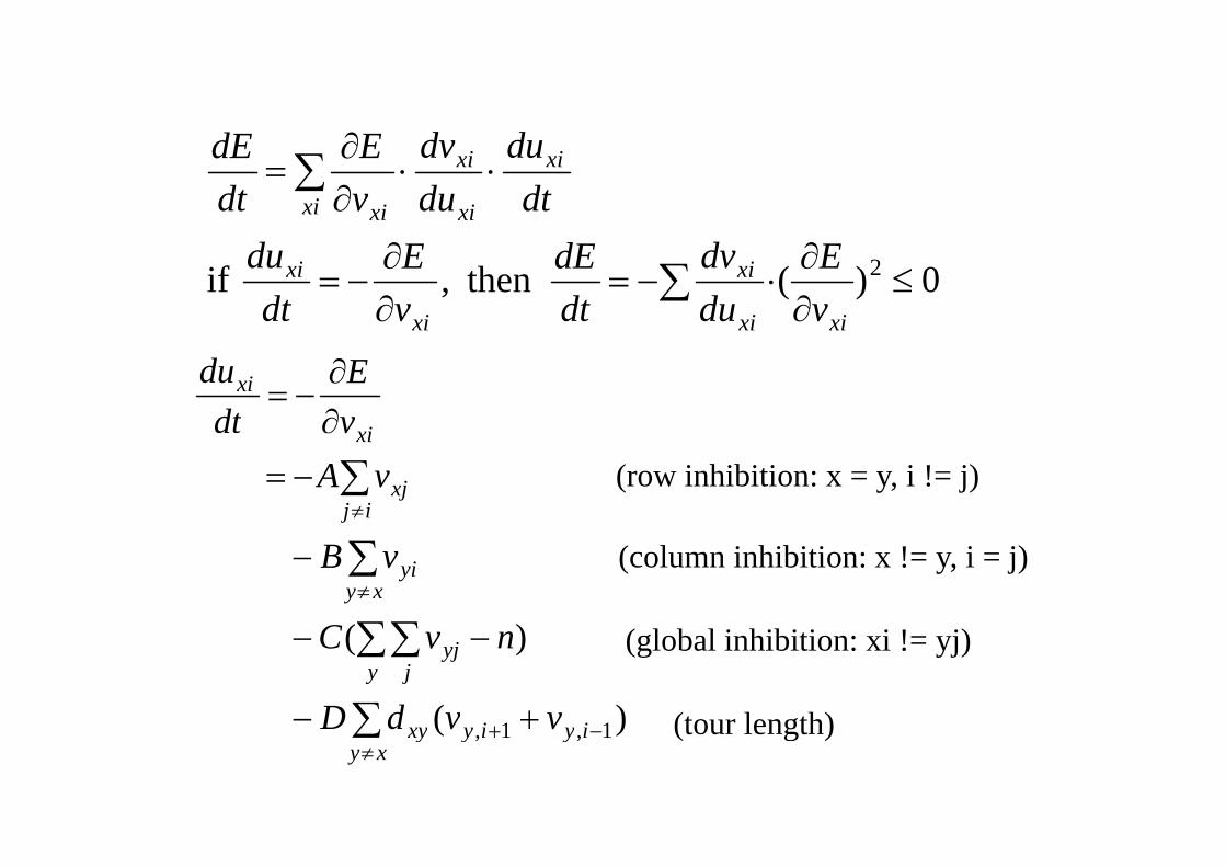
ddEdE

xi

xi

xi

xi xi dtdu

dudv

vE

dtdE

0)( then,if 2

xixi

xi

xi

xi

vE

dudv

dtdE

vE

dtdu

xi

xi

vE

dtdu

ij

xj

xi

vA (row inhibition: x = y, i != j)

xy

yi

C

vB

)(

(column inhibition: x != y, i = j)

( l b l i hibi i i ! j)

iyiyxy

y jyj

vvdD

nvC

)(

)(

11 (tour length)

(global inhibition: xi != yj)

xy

iyiyxy vvd )( 1,1, (tour length)

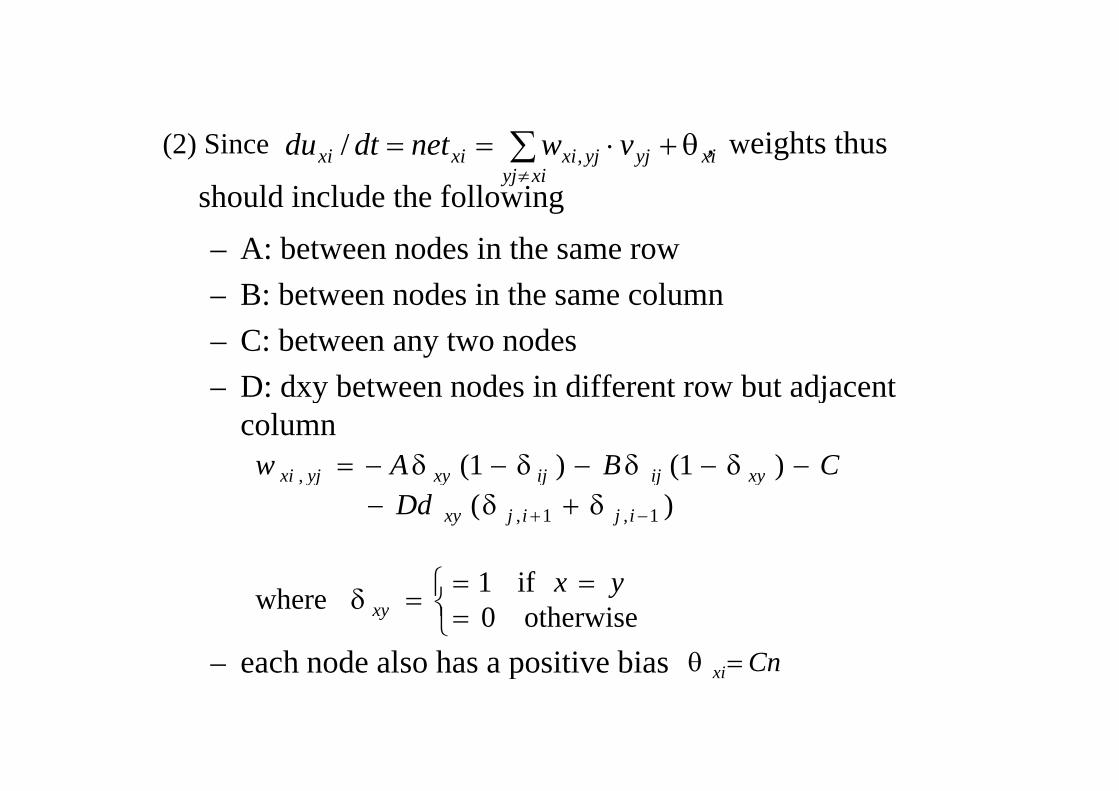
(2) Since , weights thus

should include the following

xiyj

xiyjyjxixixi vwnetdtdu ,/

– A: between nodes in the same row– B: between nodes in the same column– C: between any two nodes– D: dxy between nodes in different row but adjacentD: dxy between nodes in different row but adjacent

column)1()1(, CBAw xyijijxyyjxi

if1

)( 1,1,

Dd ijijxy

yjjyyj

– each node also has a positive bias Cn

otherwise 0if 1 where

yxxy

– each node also has a positive bias Cnxi

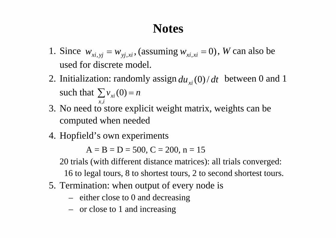
Notes

1. Since , W can also be used for discrete model

)0 (assuming , ,,, xixixiyjyjxi wwwused for discrete model.

2. Initialization: randomly assign between 0 and 1 such that

dtduxi /)0(nv )0(such that

3. No need to store explicit weight matrix, weights can be t d h d d

nvix

xi )0(,

computed when needed4. Hopfield’s own experiments

A = B = D = 500, C = 200, n = 1520 trials (with different distance matrices): all trials converged: 16 to legal tours 8 to shortest tours 2 to second shortest tours16 to legal tours, 8 to shortest tours, 2 to second shortest tours.

5. Termination: when output of every node is – either close to 0 and decreasingeither close to 0 and decreasing – or close to 1 and increasing

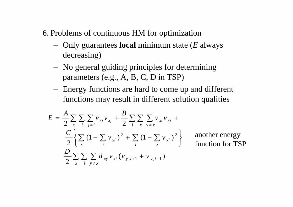
6 Problems of continuous HM for optimization6. Problems of continuous HM for optimization– Only guarantees local minimum state (E always

decreasing)decreasing)– No general guiding principles for determining

parameters (e.g., A, B, C, D in TSP)p ( g , , , , )– Energy functions are hard to come up and different

functions may result in different solution qualitiesy

i x xy

xixix i ij

xjxi vvBvvAE22

x i i xxixi

yj

D

vvC )1()1(2

22 another energy function for TSP

x i xy

iyiyxixy vvvdD )(2 1,1,

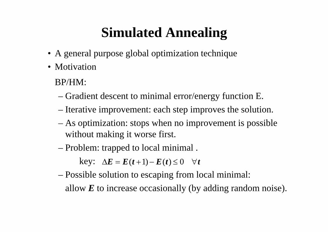
Simulated AnnealingS u ated ea g• A general purpose global optimization technique

i i• Motivation

BP/HM:– Gradient descent to minimal error/energy function E.– Iterative improvement: each step improves the solution. – As optimization: stops when no improvement is possible

without making it worse first.– Problem: trapped to local minimal .

key: ttEtEE 0)()1(– Possible solution to escaping from local minimal:

allow E to increase occasionally (by adding random noise).

Annealing Process in Metallurgy• To improve quality of metal works.• Energy of a state (a config. of atoms in a metal piece)

– depends on the relative locations between atoms.– minimum energy state: crystal lattice, durable, less fragile/crisp

many atoms are dislocated from crystal lattice causing higher– many atoms are dislocated from crystal lattice, causing higher (internal) energy.

• Each atom is able to randomly move – How easy and how far an atom moves depends on the

temperature (T), and if the atom is in right placeDislocation and other disruptions from min energy state can be– Dislocation and other disruptions from min. energy state can be eliminated by the atom’s random moves: thermal agitation.

– Takes too long if done at room temperatureg p• Annealing: (to shorten the agitation time)

– starting at a very high T, gradually reduce Tl h id f li i i i• SA: apply the idea of annealing to NN optimization

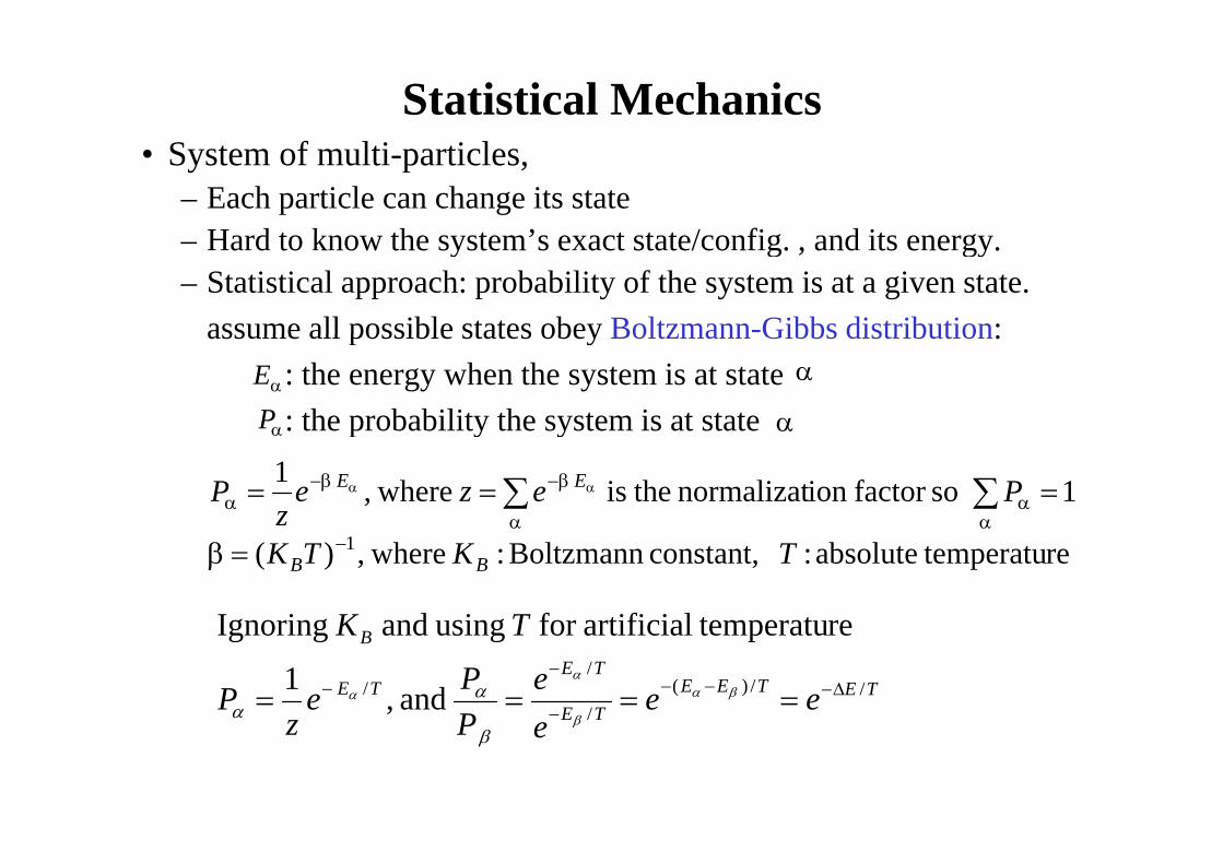
Statistical Mechanics• System of multi-particles,

– Each particle can change its state Hard to know the system’s exact state/config and its energy– Hard to know the system’s exact state/config. , and its energy.

– Statistical approach: probability of the system is at a given state.assume all possible states obey Boltzmann-Gibbs distribution:assume all possible states obey Boltzmann Gibbs distribution:

: the energy when the system is at state : the probability the system is at stateP

E

p y y

1 sofactor ion normalizat theis where,1 Pezez

P EE

re temperatuabsolute : constant,Boltzmann : where,)( 1 TKTK BB

TK retemperatuartificialforusingandIgnoring

TETEETE

TETE

B

eeee

PPe

zP

TK

//)(/

// and ,1

re temperatuartificialfor usingand Ignoring

ePz

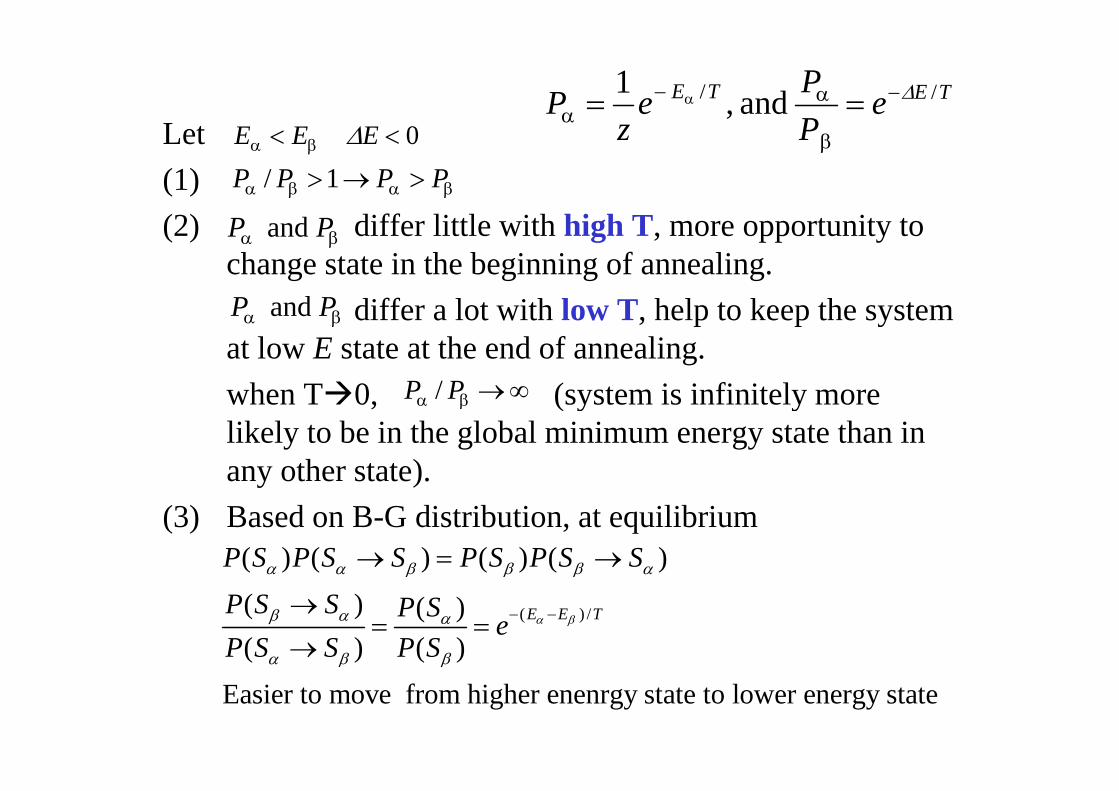
L t 0EEE

TETE ePPe

zP // and ,1

Let (1)(2) diff li l i h hi h T i

0 EEE

PPPP 1/

Pz

(2) differ little with high T, more opportunity to change state in the beginning of annealing.

differ a lot ith low T help to keep the s stem

PP and

PP and differ a lot with low T, help to keep the system at low E state at the end of annealing.when T0 (system is infinitely morePP /

PP and

when T0, (system is infinitely more likely to be in the global minimum energy state than in any other state).

PP /

y )(3) Based on B-G distribution, at equilibrium

( ) ( ) ( ) ( )P S P S S P S P S S

( ) /( ) ( )( ) ( )

E E TP S S P S eP S S P S

Easier to move from higher enenrgy state to lower energy state

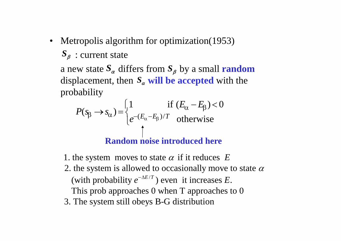
M t li l ith f ti i ti (1953)• Metropolis algorithm for optimization(1953): current state

diff f b ll dSS

Sa new state differs from by a small randomdisplacement, then will be accepted with the probability

SS

S

probability

otherwise

0)(if 1)( /)( TEEe

EEssP

otherwisee

Random noise introduced here

/

1. the system moves to state if it reduces 2. the system is allowed to occasionally move to state

E

/ (with probability ) even it increases . This prob approaches 0 when T approaches

E Te E

to 03 The system still obeys B-G distribution3. The system still obeys B-G distribution

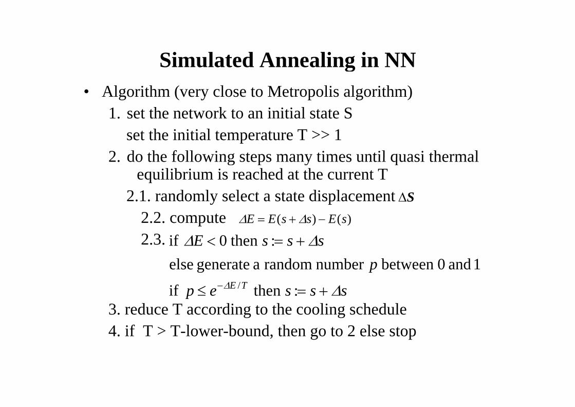
Simulated Annealing in NNSimulated Annealing in NN• Algorithm (very close to Metropolis algorithm)

1 set the network to an initial state S1. set the network to an initial state Sset the initial temperature T >> 1

2 do the following steps many times until quasi thermal2. do the following steps many times until quasi thermalequilibrium is reached at the current T

2.1. randomly select a state displacement Sy p2.2. compute 2.3.

)()( sEssEE

sssE :then0 if

sssep

pTE :thenif

1and0betweennumberrandomagenerateelse/

3. reduce T according to the cooling schedule4. if T > T-lower-bound, then go to 2 else stop

p

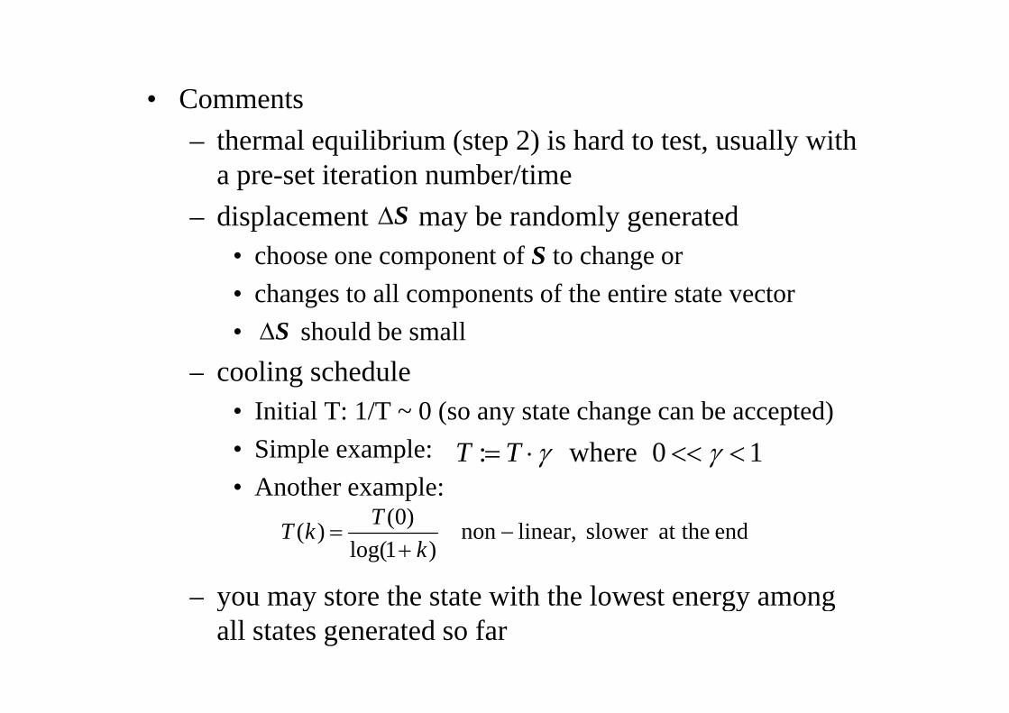
• Comments– thermal equilibrium (step 2) is hard to test, usually with

a pre-set iteration number/time– displacement may be randomly generated

• choose one component of S to change or S

• changes to all components of the entire state vector• should be smallS

– cooling schedule• Initial T: 1/T ~ 0 (so any state change can be accepted) • Simple example:• Another example:

: where 0 1T T

)0(T

– you may store the state with the lowest energy among

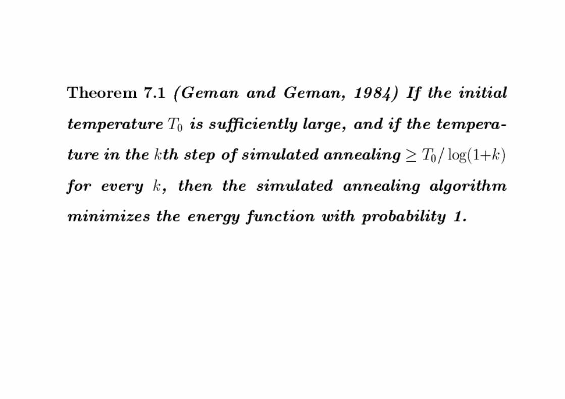
endtheatslower linear,non)1log(

)0()(

k

TkT

you may store the state with the lowest energy among all states generated so far

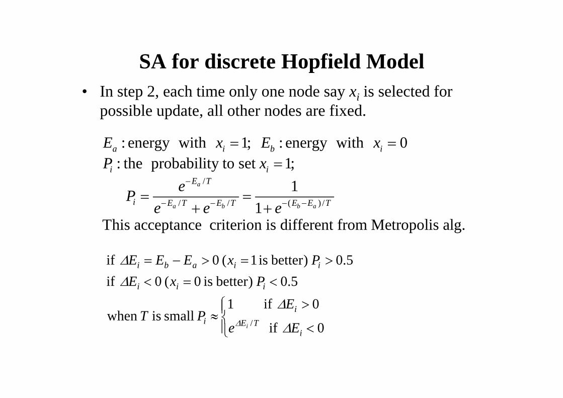
SA for discrete Hopfield ModelSA for discrete Hopfield Model• In step 2, each time only one node say xi is selected for

possible update all other nodes are fixedpossible update, all other nodes are fixed.

: energy with 1; : energy with 0a i b iE x E x

/

: the probability to set 1; 1a

i iE T

P xeP

/ / ( ) / 1

This acceptance criterion is different from Metropolis alg.a b b ai E T E T E E TP

e e e

5.0)betteris0(0if5.0)betteris1(0if

iii

iiabi

PxEPxEEE

0if

0if 1smalliswhen /

iTE

ii

iii

Ee

EPT

i

i

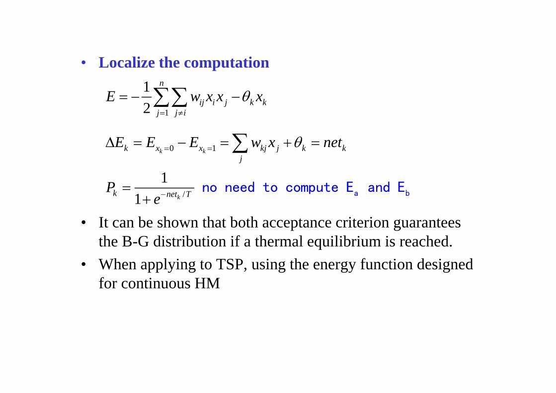
• Localize the computation• Localize the computation12

n

ij i j k kE w x x x 1

0 1

2

k k

j j i

k x x kj j k kE E E w x net

/

11

k k

k

j jj

k net TP

a bno need to compute E and E

• It can be shown that both acceptance criterion guarantees the B G distribution if a thermal equilibrium is reached

/1 knet Te

the B-G distribution if a thermal equilibrium is reached.• When applying to TSP, using the energy function designed

for continuous HMfor continuous HM

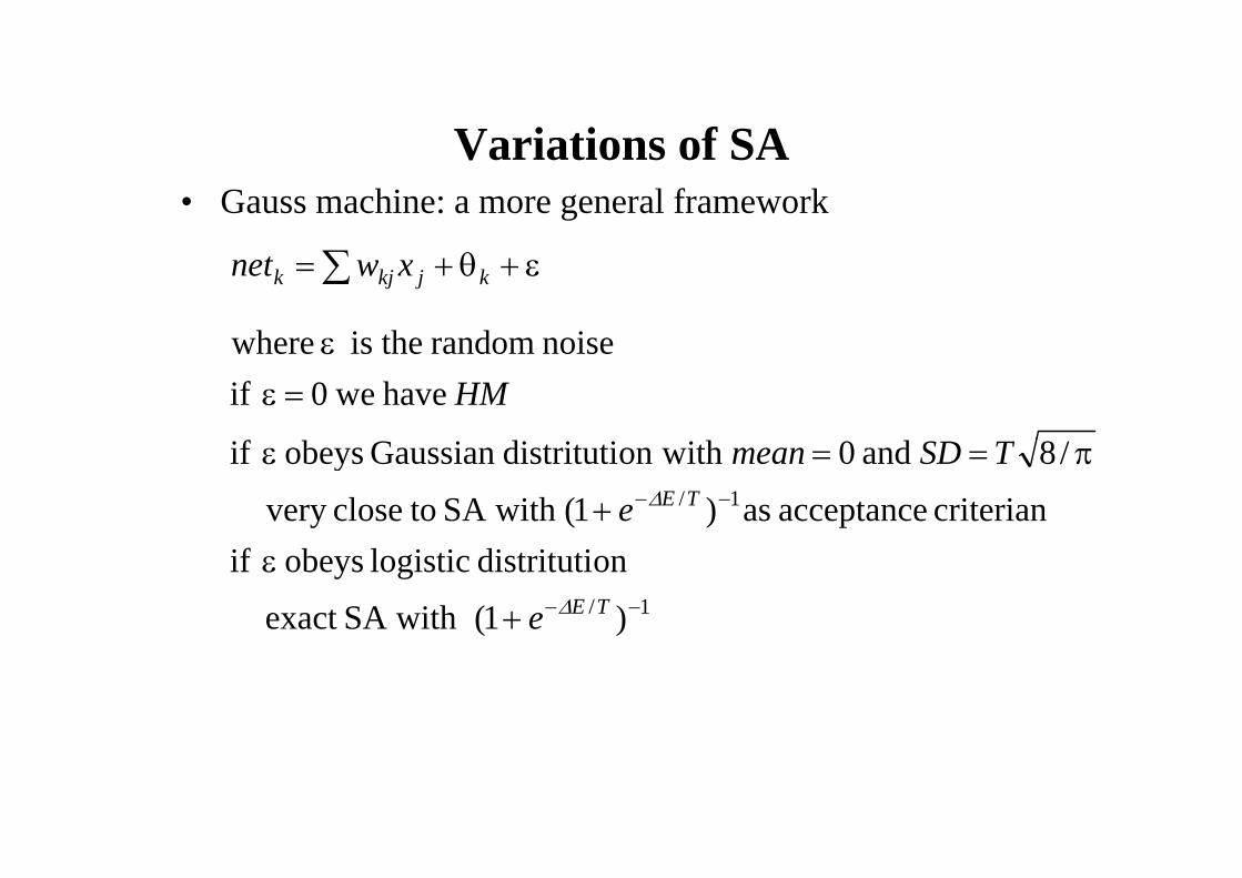
Variations of SAVariations of SA• Gauss machine: a more general framework

noiserandomtheiswhere

kjkjk xwnet

havewe0ifnoiserandomtheis where

HM

1/ criterianacceptanceas)1(withSAtoclosevery

/8and0withondistritutiGaussianobeysif

TEe

TSDmean

1/ )1(withSAexact

ondistritutilogisticobeysif

TEe

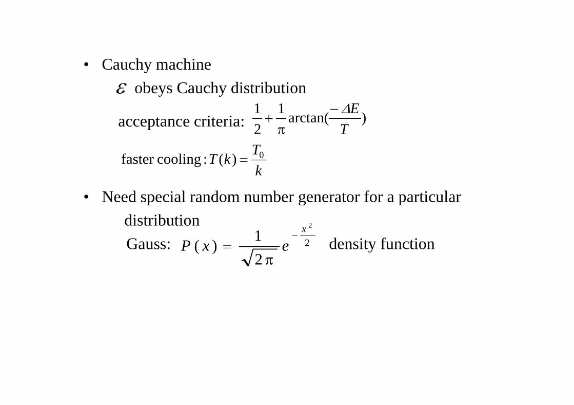
• Cauchy machine• Cauchy machineobeys Cauchy distribution

11 Eacceptance criteria: )arctan(1

21

TE

TkT 0)(lif t

• Need special random number generator for a particular k

kT 0)(:coolingfaster

p g pdistributionGauss: density function2

2

1)(x

exP

Gauss: density function2

)( exP

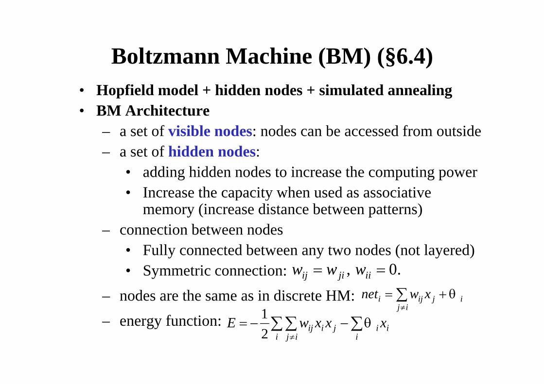
Boltzmann Machine (BM) (§6.4)Boltzmann Machine (BM) (§6.4) • Hopfield model + hidden nodes + simulated annealing• BM Architecture

– a set of visible nodes: nodes can be accessed from outsidet f hidd d– a set of hidden nodes:

• adding hidden nodes to increase the computing power• Increase the capacity when used as associative• Increase the capacity when used as associative

memory (increase distance between patterns)– connection between nodes

• Fully connected between any two nodes (not layered)• Symmetric connection: .0, iijiij www

– nodes are the same as in discrete HM: – energy function:

jj

ij

ijiji xwnet

xxxwE 1energy function:

i ij i

iijiij xxxwE2

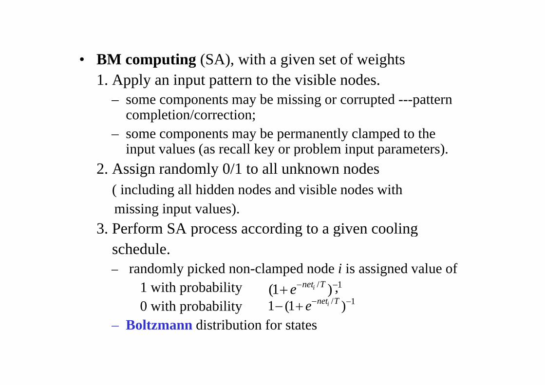
• BM computing (SA) with a given set of weightsBM computing (SA), with a given set of weights1. Apply an input pattern to the visible nodes.

– some components may be missing or corrupted ---pattern p y g p pcompletion/correction;

– some components may be permanently clamped to the input values (as recall key or problem input parameters)input values (as recall key or problem input parameters).

2. Assign randomly 0/1 to all unknown nodes( including all hidden nodes and visible nodes with( including all hidden nodes and visible nodes withmissing input values).

3. Perform SA process according to a given coolingp g g gschedule.– randomly picked non-clamped node i is assigned value of

1 with probability , 0 with probability

Boltzmann distribution for states

1/ )1( Tnetie1/ )1(1 Tnetie

– Boltzmann distribution for states

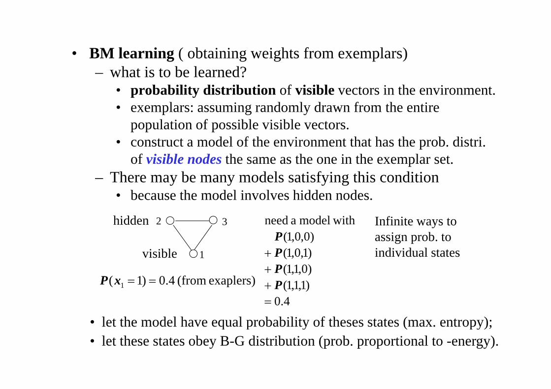
• BM learning ( obtaining weights from exemplars)– what is to be learned?

• probability distribution of visible vectors in the environment. • exemplars: assuming randomly drawn from the entire• exemplars: assuming randomly drawn from the entire

population of possible visible vectors.• construct a model of the environment that has the prob. distri.

of visible nodes the same as the one in the exemplar set.– There may be many models satisfying this condition

• because the model involves hidden nodes• because the model involves hidden nodes.

32hidden)001(

withmodel a needP

Infinite ways to assign prob to

1visible

)111()0,1,1()1,0,1()0,0,1(

PPPP

exaplers)(from40)1( 1 xP

assign prob. to individual states

• let the model have equal probability of theses states (max. entropy);4.0

)1,1,1( Pexaplers)(from4.0)1( 1xP

q p y ( py);• let these states obey B-G distribution (prob. proportional to -energy).

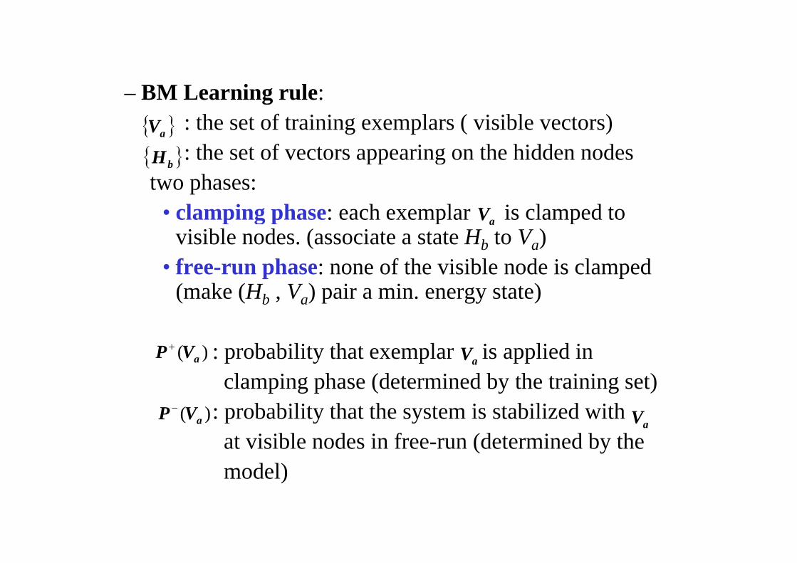
BM Learning rule:– BM Learning rule:: the set of training exemplars ( visible vectors): the set of vectors appearing on the hidden nodes

aV

H : the set of vectors appearing on the hidden nodestwo phases:

• clamping phase: each exemplar is clamped to

bH

Vclamping phase: each exemplar is clamped to visible nodes. (associate a state Hb to Va)

• free-run phase: none of the visible node is clamped

aV

(make (Hb , Va) pair a min. energy state)

b bilit th t l i li d i)( : probability that exemplar is applied inclamping phase (determined by the training set)

: probability that the system is stabilized with

)( aVP

)(VP

aV

: probability that the system is stabilized with at visible nodes in free-run (determined by the model)

)( aVPaV

model)

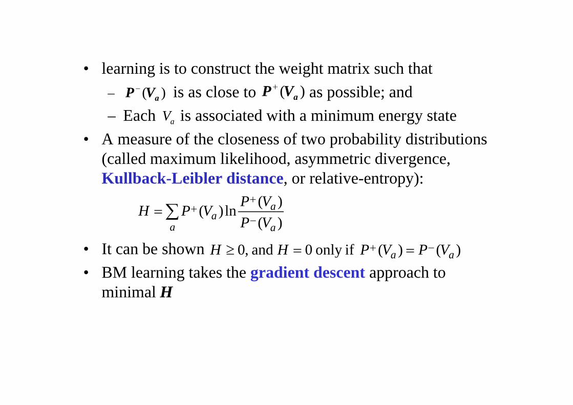
l i i t t t th i ht t i h th t• learning is to construct the weight matrix such that – is as close to as possible; and

E h i i d i h i i)( aVP )( aVP

– Each is associated with a minimum energy state• A measure of the closeness of two probability distributions

(called ma im m likelihood as mmetric di ergence

aV

(called maximum likelihood, asymmetric divergence, Kullback-Leibler distance, or relative-entropy):

VP )(

• It can be shown

a a

aa VP

VPVPH)()(ln)(

)()(ifonly0and0 VPVPHH • It can be shown• BM learning takes the gradient descent approach to

minimal H

)()(ifonly0and,0 aa VPVPHH

minimal H

/

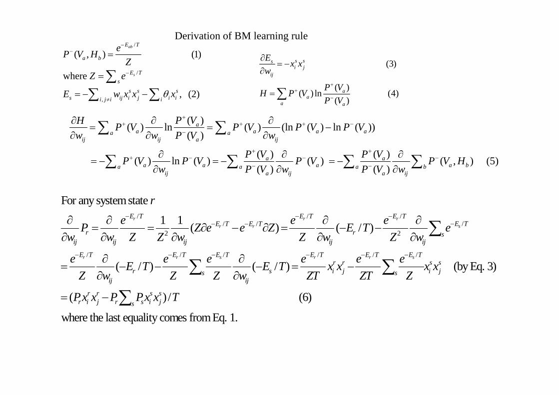
( , ) (1)abE T

a beP V H

Z

Derivation of BM learning rule

(3)s ssE x x/

,

where

, (2)

sE Ts

s s ss ij i j i ii j i i

ZZ e

E w x x x

(3)

( )( ) ln (4)( )

si j

ij

aa

a a

x xw

P VH P VP V

( )( ) ln ( ) (ln ( ) ln ( ))( )

( ) ( )

aa a a aa a

ij ij a ij

P VH P V P V P V P Vw w P V w

P V P V

( ) ( ) ( ) ln ( ) ( ) ( , ) (5)( ) ( )

a aa a a a ba a a b

ij a ij a ij

P V P VP V P V P V P V Hw P V w P V w

F t t t/ / /

// /2 2

For any system state 1 1 ( ) ( / )

r r rsr r

E T E T E TE TE T E T

r r sij ij ij ij ij

re e eP Z e e Z E T e

w w Z Z w Z w Z w

/ // / / /

( / ) ( / )s sr r r r

ij ij ij ij ij

E T E TE T E T E T E Tr r s s

r s i j i js sij ij

e e e e e eE T E T x x x xZ w Z Z w ZT ZT Z

(by Eq. 3)

( ) / (6)

where the last equality comes from Eq. 1.

r r s sr i j r s i js

Px x P Px x T

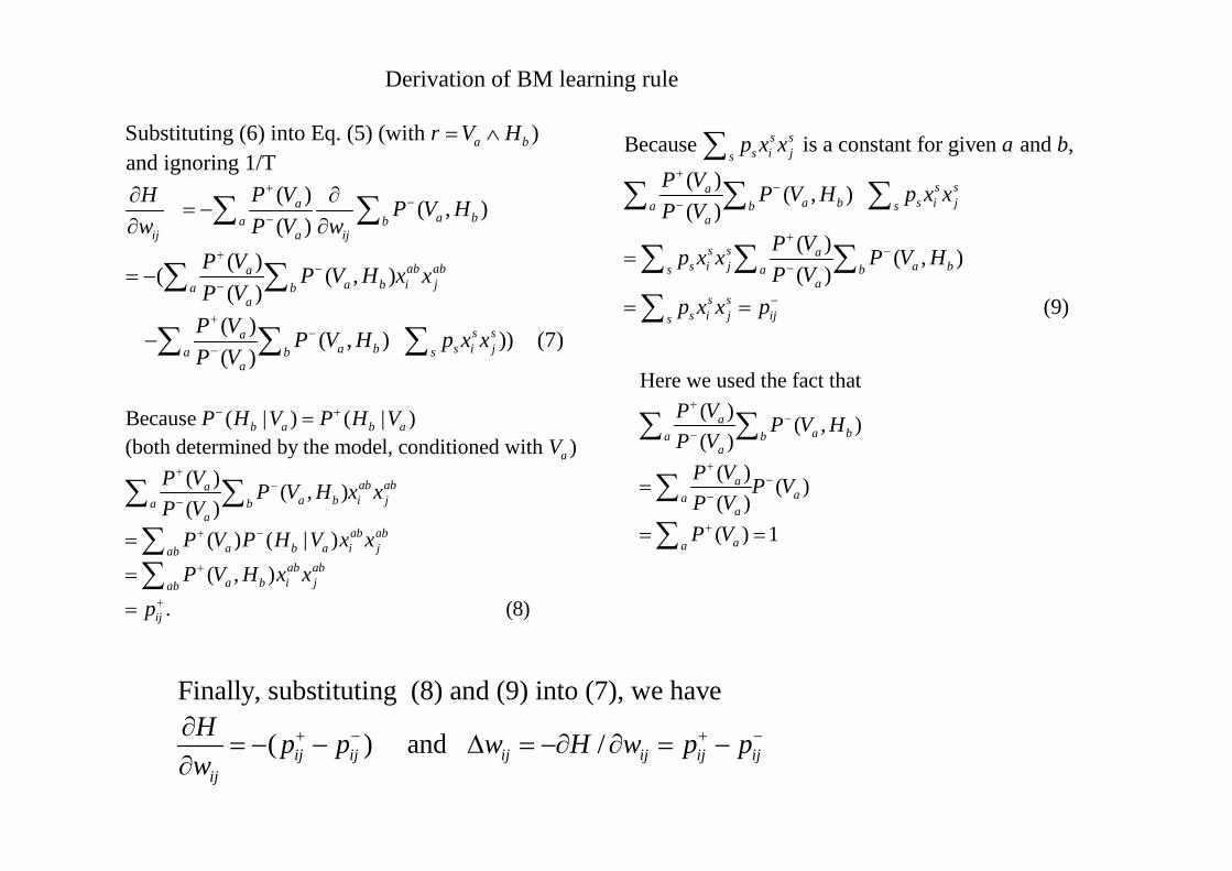
Derivation of BM learning rule

Substituting (6) into Eq. (5) (with )br V H B i t t f i ds s bSubstituting (6) into Eq. (5) (with )and ignoring 1/T

( ) ( , ) ( )

a b

aa ba b

ij a ij

r V H

P VH P V Hw P V w

Because is a constant for given and ,( ) ( , )( )

( )

s ss i js

s saa b s i ja b s

a

p x x a bP V P V H p x xP V

P V

( )( )( ( , )( )

( ) ( ) )) (7)

ij a ij

ab abaa b i ja b

a

s sa

P V P V H x xP V

P V P V H

( ) ( , )( )

(9)

s s as i j a bs a b

as s

s i j ijs

P Vp x x P V HP V

p x x p

( ) ( , ) )) (7)

( )s sa

a b s i ja b sa

P V H p x xP V

Because ( | ) ( | )b a b aP H V P H V

Here we used the fact that ( ) ( , )( )

aa ba b

P V P V HP V

(both determined by the model, conditioned with )

( ) ( , )( )

( ) ( | )

a

ab abaa b i ja b

aab ab

VP V P V H x xP V

P V P H V

( )( )

( ) ( )( )( ) 1

a ba ba

aaa

a

P VP V P VP VP V

( ) ( | )

( , ). (8)

ab aba b a i jab

ab aba b i jab

ij

P V P H V x xP V H x x

p

( ) 1aaP V

Finally, substituting (8) and (9) into (7), we haveH ( ) and /ij ij ij ij ij ij

ij

H p p w H w p pw

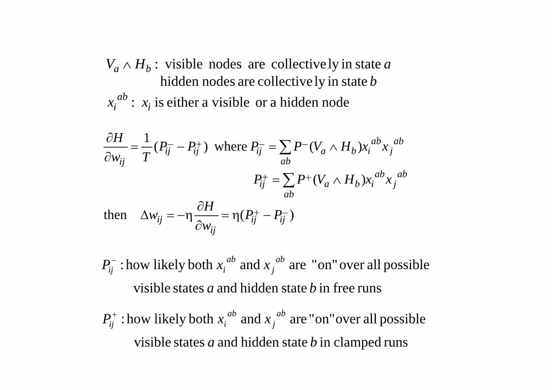
stateinlycollectivearenodesvisible: aHV

nodehiddenaorvisibleaeitheris: statein ly collective are nodeshidden

statein ly collective are nodes visible :

iab

i

ba

xxb

aHV

)( where)(1

abj

abibaijijij xxHVPPPPH

nodehidden aor visibleaeither is : ii xx

)(

)()(

ab

jab

iab

baij

jiab

baijijijij

xxHVPP

VTw

)(then

ijijij

ij

ab

PPwHw

fihidddi ibl

possible allover on"" are and both likely how :

b

xxP abj

abiij

runsfreein statehidden andstatesisible v ba

possible allover on"" are and both likely how : xxP abj

abiij

runs clampedin statehidden and states isible v bajj

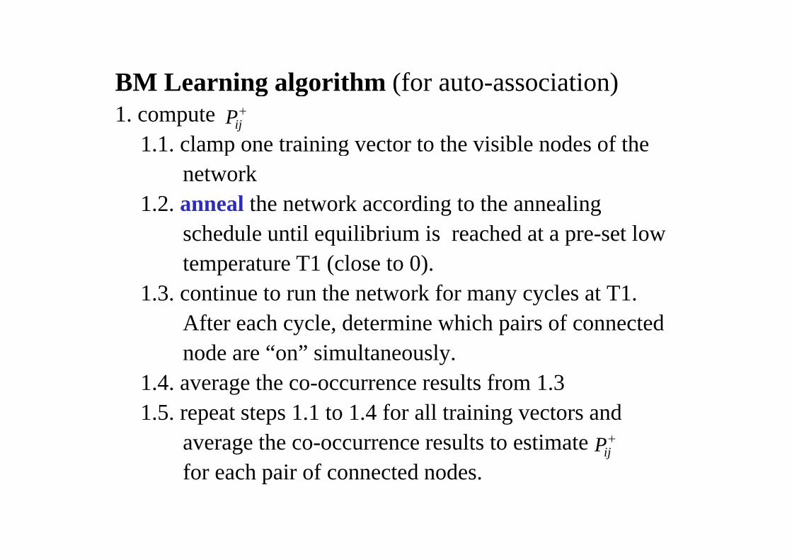
BM Learning algorithm (for auto-association)BM Learning algorithm (for auto association)1. compute

1.1. clamp one training vector to the visible nodes of the

ijPp g

network1.2. anneal the network according to the annealing

schedule until equilibrium is reached at a pre-set lowtemperature T1 (close to 0).

1.3. continue to run the network for many cycles at T1. After each cycle, determine which pairs of connected node are “on” simultaneously.

1.4. average the co-occurrence results from 1.31 5 t t 1 1 t 1 4 f ll t i i t d1.5. repeat steps 1.1 to 1.4 for all training vectors and

average the co-occurrence results to estimate for each pair of connected nodes

ijP

for each pair of connected nodes.

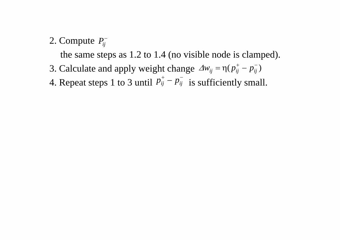
2 C t P2. Computethe same steps as 1.2 to 1.4 (no visible node is clamped).

3 C l l d l i h h )(

ijP

3. Calculate and apply weight change4. Repeat steps 1 to 3 until is sufficiently small.

)( ijijij ppw ijij pp

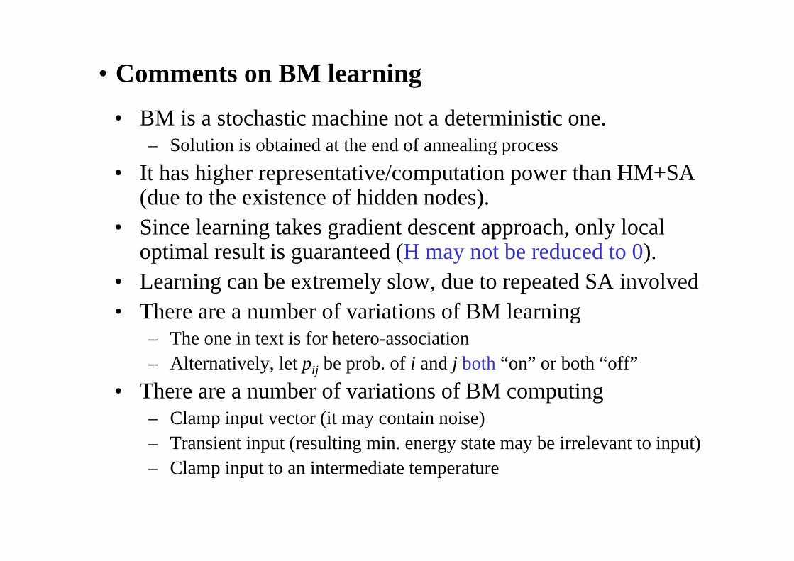
• Comments on BM learning

• BM is a stochastic machine not a deterministic one.– Solution is obtained at the end of annealing processg p

• It has higher representative/computation power than HM+SA (due to the existence of hidden nodes).

• Since learning takes gradient descent approach, only local optimal result is guaranteed (H may not be reduced to 0).

• Learning can be extremely slow due to repeated SA involved• Learning can be extremely slow, due to repeated SA involved• There are a number of variations of BM learning

– The one in text is for hetero-associationThe one in text is for hetero association– Alternatively, let pij be prob. of i and j both “on” or both “off”

• There are a number of variations of BM computing– Clamp input vector (it may contain noise)– Transient input (resulting min. energy state may be irrelevant to input)– Clamp input to an intermediate temperatureClamp input to an intermediate temperature

• Comments on BM learning

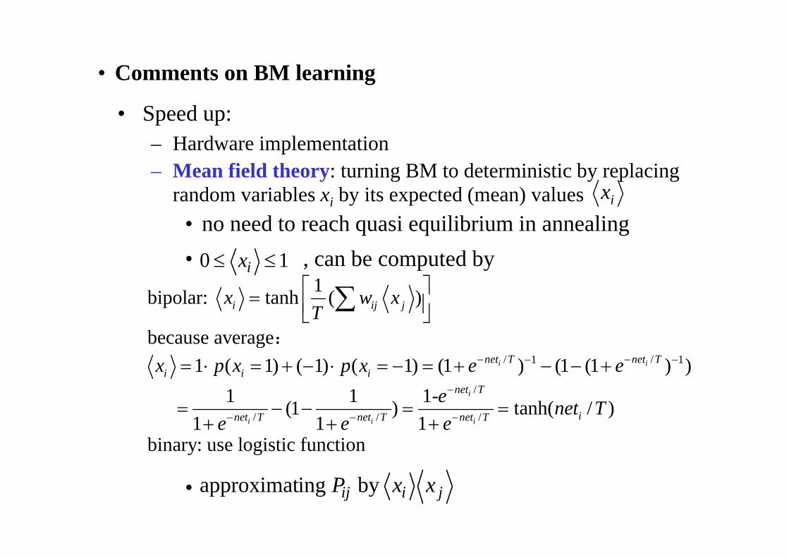
• Speed up:– Hardware implementationp– Mean field theory: turning BM to deterministic by replacing

random variables xi by its expected (mean) valuesd h i ilib i i li

ix • no need to reach quasi equilibrium in annealing• , can be computed by10 ix

1 1bipolar: tanh ( )

because average

i ij jx w xT

：

/ /1 1

/

because average 1 ( 1) ( 1) ( 1) (1 ) (1 (1 ) )

1 1 1-(1 ) tanh( / )

i i

i

net T net Ti i i

net T

x p x p x e ee t T

：

/ / / (1 ) tanh( / )1 1 1

binary: use logistic funi i i inet T net T net T net T

e e e

ction

• jiij xxP by ingapproximat

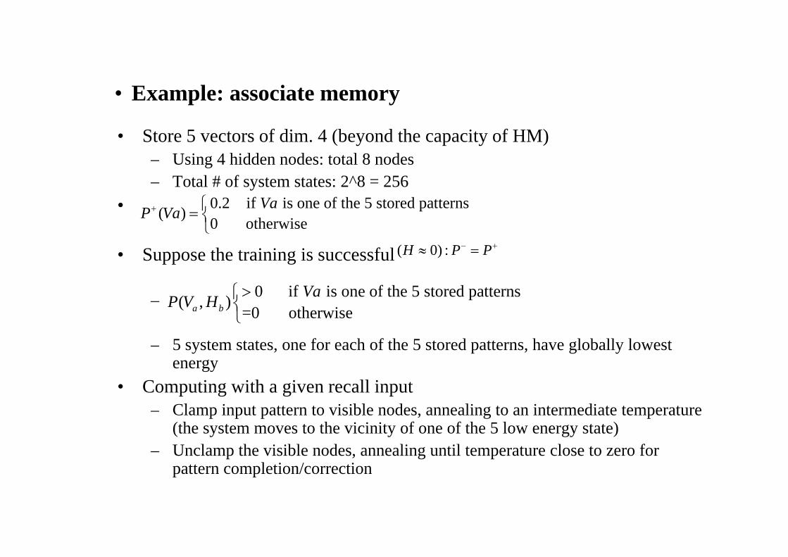
E l i t• Example: associate memory

• Store 5 vectors of dim. 4 (beyond the capacity of HM)– Using 4 hidden nodes: total 8 nodes– Total # of system states: 2^8 = 256

• 0.2 if is one of the 5 stored patterns( ) VaP Va

• Suppose the training is successful

( )0 otherwise

P Va

( 0) :H P P

–

5 t t t f h f th 5 t d tt h l b ll l t

0 if is one of the 5 stored patterns( , )=0 otherwisea b

VaP V H

– 5 system states, one for each of the 5 stored patterns, have globally lowest energy

• Computing with a given recall inputCl i i ibl d li i di– Clamp input pattern to visible nodes, annealing to an intermediate temperature (the system moves to the vicinity of one of the 5 low energy state)

– Unclamp the visible nodes, annealing until temperature close to zero for pattern completion/correctionpattern completion/correction

Evolutionary Computing (§7.5)Evolutionary Computing (§7.5)• Another expensive method for global optimization• Stochastic state-space search emulating biological

evolutionary mechanisms– Biological reproduction

• Most properties of offspring are inherited from parents, each parent contributes different part of the offspring’s chromosome/gene structure (cross-over)

• Some are resulted from random perturbation of gene• Some are resulted from random perturbation of gene structures (mutation)

– Biological evolution: survival of the fittestBiological evolution: survival of the fittest• Individuals of greater fitness have more offspring• Genes that contribute to greater fitness are more predominant g p

in the population

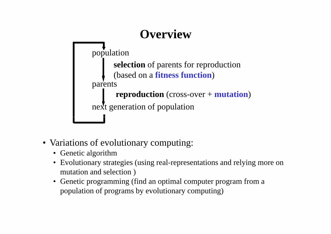
Overviewpopulation

selection of parents for reproduction

Overview

selection of parents for reproduction (based on a fitness function)

parentsreproduction (cross-over + mutation)

next generation of population

• Variations of evolutionary computing:• Variations of evolutionary computing:• Genetic algorithm• Evolutionary strategies (using real-representations and relying more on

t ti d l ti )mutation and selection )• Genetic programming (find an optimal computer program from a

population of programs by evolutionary computing)

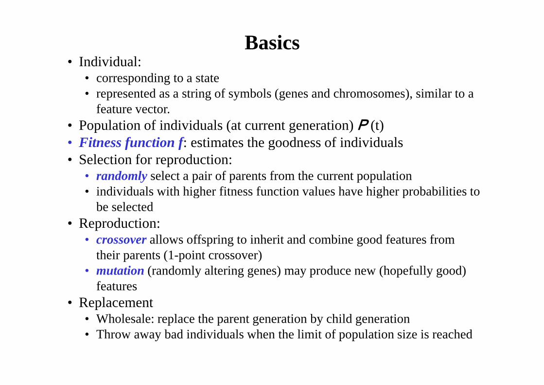
• Individual:Basics

• Individual: • corresponding to a state• represented as a string of symbols (genes and chromosomes), similar to a

ffeature vector.• Population of individuals (at current generation) P (t)• Fitness function f: estimates the goodness of individualsf f g• Selection for reproduction:

• randomly select a pair of parents from the current population• individuals with higher fitness function values have higher probabilities to• individuals with higher fitness function values have higher probabilities to

be selected• Reproduction:

ll ff i t i h it d bi d f t f• crossover allows offspring to inherit and combine good features from their parents (1-point crossover)

• mutation (randomly altering genes) may produce new (hopefully good) features

• Replacement• Wholesale: replace the parent generation by child generationp p g y g• Throw away bad individuals when the limit of population size is reached

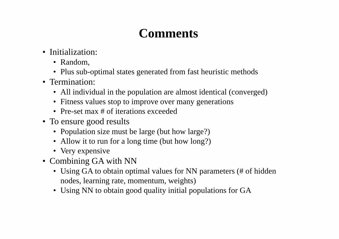
Comments• Initialization:

• Random, ,• Plus sub-optimal states generated from fast heuristic methods

• Termination:• All individual in the population are almost identical (converged)• All individual in the population are almost identical (converged)• Fitness values stop to improve over many generations • Pre-set max # of iterations exceeded

T d lt• To ensure good results• Population size must be large (but how large?)• Allow it to run for a long time (but how long?)• Very expensive

• Combining GA with NN• Using GA to obtain optimal values for NN parameters (# of hidden g p p (

nodes, learning rate, momentum, weights)• Using NN to obtain good quality initial populations for GA