Chapter 7

Least Squares Optimal Scaling of Partially Observed Linear Systems

Jan DeLeeuw

University of California at Los Angeles, Department of Statistics. Los Angeles, USA

7.1 Introduction

7.1.1 Problem We compute approximate solutions to homogeneous linear systems of the form AB = 0. Here B is an m x p matrix, and A is an n x m matrix. Columns of A correspond with variables, rows with observations. Columns of B correspond with equations connecting the variables, elements of B are coefficients.

Both A and B are, in general, partially known and our job is to impute the unknown elements. Unknown information on the variable side can be the usual missing data, it can be in the form of unobserved (latent) variables, or it can be in the form of allowing for transformations of the variables.

Our fit criterion will be least squares. This is different from the usual procedure, which embeds the data in a statistical model and then applies some form of maximum likelihood. In particular, in the classical case, it is assumed that the rows of A are replications of a random vector f!, which satisfies g'B = 0. We then transform the system to B'"'£B = 0, where "'£ = E(f!q~, and we proceed to estimate "'£ under these constraints, and maybe other constraints as well (often assuming multivariate normality of f! and often integrating out the parts corresponding with missing information).

121

K. van Montfon eta/. (eds.), Recent Developments on Structural Equation Models. 121-134. © 2004 Kluwer Academic Publishers.

122 JanDe Leeuw

This may be fine in some situations, although in non-normal situations it is unclear why one should focus on the covariances. But in other situations the repeated independent trials assumption does not make sense, using random variables is not natural, assuming multivariate normality is ludicrous, and the framework leads to very complicated or even impossible estimation problems. We suggest a more direct approach, formulated directly in terms of the obser­vations, and using least squares to solve matrix approximation problems.

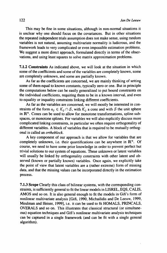
7.1.2 Constraints As indicated above, we will look at the situation in which some of the coefficients and some of the variables are completely known, some are completely unknown, and some are partially known.

As far as the coefficients are concerned, we are mainly thinking of setting some of them equal to known constants, typically zero or one. But in principle the computations below can be easily generalized to put bound constraints on the individual coefficients, requiring them to be in a known interval, and even to equality or inquality constraints linking different coefficients.

As far as the variables are concerned, we will mostly be interested in con­straints of the form ai E lCj n S, with !Ci a cone and with S the unit sphere in Rn. Cones can be used to allow for monotone transformations, spline sub­spaces, or monotone splines. For variables we will also explicitly discuss more complicated linking constraints, in particular we often require orthogonality of different variables. A block of variables that is required to be mutually orthog­onal is called an orthoblock.

A key component of our approach is that we allow for variables that are completely unknown, i.e. their quantifications can be anywhere in R n. Of course, we need to have some prior knowledge in order to prevent perfect but trivial solutions to our system of equations. These unknown or latent variables will usually be linked by orthogonality constraints with other latent and ob­served (known or partially known) variables. Once again, we explicitly take the point of view that latent variables are a (rather extreme) form of missing data, and that the missing values can be incorporated directly in the estimation process.

7 .1.3 Scope Clearly this class of bilinear systems, with the corresponding con­straints, is sufficiently general to fit the linear models in LISREL, EQS, CALIS, AMOS and so on. It is also general enough to fit the models in Gift's form of nonlinear multivariate analysis [Gifi, 1990, Michailidis and DeLeeuw, 1999, Meulman and Heiser, 1999], i.e. it can be used to fit HOMALS, PRINCALS, OVERALS and so on. This illustrates that classical structural (or simultane­ous) equation techniques and Gift's nonlinear multivariate analysis techniques can be captured in a single framework (and can be fit with a single general algorithm).

Least Squares Optimal Scaling of Partially Observed Unear Systems 123

7 .1.4 Equivalent Systems In most cases we can rewrite the system, still in the required linear form, in such a way that the rewritten systems has the same solutions set as the original system. This does not mean, however, that the least squares solutions to the rewritten and the original system are the same. We shall see some examples of equivalent system of linear equations below. A classical example is the reduced form of simultaneous equation systems.

7 .1.5 Generalizations Most of the developments below go through without modifications if we use weighted least squares, with known weights, instead of unweighted least squares. Similarly, variables can be elements of an arbi­trary inner product space, instead of vectors in R n. Thus we can use sample or population distributions to compute the inner products of our variables, to study what happens in the population case, or to find out what sampling distri­butions of our statistics are.

We will not elaborate further on these easy generalizations, but it is good to remember that they are available at little cost.

7.2 Loss Function and Algorithm

7 .2.1 Loss Function The problem studied in this paper is to minimize the least squareslossjUnction

a( A, B) = tr B' RB. Here R = A' A is the m x m correlation matrix of the variables.

Thus, we will look at the general class of problems in which we minimize a(A, B) over the A satisfying cone and orthogonality restrictions and over the B with some of the elements known.

7.2.2 Algorithm In DeLeeuw [1990], we studied the problem of minimizing any real-valued function of the form </>(R), with R = A' A, over a; E K.; n S. A majorization algorithm [DeLeeuw, 1994, Heiser, 1995, Lange et al., 2000] was developed there for the case in which <P(R) is concave in R. Futher developments of this approach are in DeLeeuw [1988, 1993] and in DeLeeuw et at. [1999].

In the problem studied in this paper we can define

¢(R) =min tr B' RB, BEB

where Bare the matrices in Rmxp satisfying the constraints on B. The loss function </> is the pointwise minimum of a family of functions linear, and thus concave, in R. Because the pointwise minimum of a family of concave func­tions is also concave, it follows that ¢ is concave in R. We have seen that the

124 Jan DeLeeuw

majorization algorithm applies to concave functions, and thus </> can be min­imized by the majorization algorithm. In that sense the class of techniques discussed here is an important (and so far unexplored) special case of our pre­vious work. The main generalization is that in the current framework we do not only have the cone constraints on individual variables, but we also allow for orthoblocks of variables.

We give a brief outline of the algorithm in the general case. Algorithms for specific systems will be discussed in more detail below. For the majorization algorithm we need the subgradient of the loss function. For </> the subgradient 8</>( R) is the convex hull of the matrices iJ B', where iJ is any matrix minimiz­ing tr B' RB over B E 8. This follows from the formula for the subgradient of a pointwise minimum of concave functions [Hiriart-Urruty and Lemarechal, 1993, Theorem 4.4.2]. Observe that computing iJ is a quadratic minimization problem. This is why it is easy to incorporate bound and linear inequality con­straints on the coefficients, because we will remain in the convex quadratic programming framework.

The subgradient inequality tells us that </>( R) ~ tr RG, for any G E 8</>(R). The algorithm selects a subgradient G, and minimizes the majorization function tr RG by cycling over all variables (or orthoblocks of variables). This gives us a new R+, and we have

In majorization theory this is called the sandwich inequality, and it forces con­vergence of the sequence of loss function values (and through that, using Zang­will [1969], convergence of the sequence of solutions). Observe that conver­gence will be to a stationary point of the algorithm, which is a point satisfying the stationary equations of the minimization problem. This is likely to be a lo­cal minimum, because it is a minimum with respect to each block of variables, but there is no guarantee that we find the global minimum.

Observe that if we update a variable, or an orthoblock, we have to recom­pute the subgradient at the new point, i.e. we have to recompute the optimal B for current A, before we proceed to the next variable or block.

7 .2.3 Subproblems for Variables Suppose we are optimizing over the single variable a1 E 1\:1 n S, keeping A2 , the rest of A, fixed at its current values. Partition A and G in the obvious way. Then

tr RG = g11 + 2a~A2g1 + tr A~A2G22·

Only the second term depends on a 1. DeLeeuw [1990] shows that the new optimal a1 can be found by projecting h = A2g1 on the cone 1\:1 and then normalizing the projection to unit length.

Least Squares Optimal Scaling of Partially Observed Linear Systems 125

If we are optimizing over an orthoblock of variables AI, then by the same reasoning

tr RG = tr Gu + 2tr A~A2GI2 + tr A~A2G22·

Thus the optimal AI is found by solving the orthogonal Procrustus problem for ii = A2GI2• If ii has full column rank, and ii = KAL' is its singular value decomposition, then the optimal AI is K L'. In the Appendix we generalize this to singular ii, a generalization we will need in our factor analysis algorithm.

We discuss two more subproblems we can come across in implementing the general algorithm. First, we want to find ai E JCI n S orthogonal to the block A2, but not necessarily to the block A3 . Clearly

tr RG = a~ A2g2 + a~ A3g3 + terms not dependent on a I

To find the optimal ai we need to project

h = (I- A2(A~A2)-I A~)Aa9a

on JC1o and normalize. We do not assume here that A2 is an orthoblock. The second subproblem asks for an orthoblock AI which is orthogonal to

block A2, but not necessarily to block A3. With the same reasoning as in the previous subproblem, we now have to apply Procrustus to

ii =(I- A2 (A~A2)-IA~)A3Gai·

7 .2.4 Algorithm Flow The flow of the algorithm is to partition A into blocks that are either orthoblocks or single variables. We optimize the variables over the first block, optimize over B, optimize variables in the second block, opti­mize over B, and so on. It is not necessary to go through the blocks of vari­ables in order, in fact we can change the order or use "free-steering" meth­ods in which we cycle through the blocks in random order [DeLeeuw and Michailides, 1999], but in general it is necessary to update B every time we update a block of variables. This may be inefficient if computing B is much more complicated than updating blocks of variables. There are variations of the algorithm possible based on using majorization a second time, this time to bound.

It is sometimes also possible, and even advisable, to decompose B into a number of blocks and apply block relaxation to optimize over B. Thus many variations are possible with our general "algorithm model".

126 JanDe Leeuw

7.3 Examples

Let us look at some "classical " systems to see how they fit into our framework and to see what loss functions and algorithms we can expect to discover (or rediscover). In discussing regression and various other special cases of our general framework, we use additional notation which is natural for the problem at hand and consequently obvious.

7.3.1 Regression It has always been somewhat ambiguous what regression analysis wants of the residuals. On the one hand, we want the residuals to be "small", on the other hand we want them to be "unsystematic", which means unrelated to the predictors (and may mean more). Clearly being small does not imply being unsystematic, and vice versa.

This means that we can distinguish two regression problems in our frame­work. The first system is

or y = X j3 + ae, where we require e' X = 0. Minimizing loss gives the usual regression statistics (regression coeffi­

cients, residuals, residual sum of squares), which actually make the minimum loss equal to zero. There is no room for improvement of the loss in this case by using optimal cone transformations of the variables. If we have missing in­formation in X and/or y, we can just fill it in arbitrarily, and we will still have zero loss. This simply repeats the obvious: if we project a vector orthogonally on a subspace then the residuals are orthogonal to the subspace, and thus the decomposition we seek is always possible.

Now let us "ignore emors", i.e. remove e from the system. We concentrate on making the residuals smalL Thus

The solution for {3, for given X and y, is again the usual vector of regression coefficients, but now, of course, the minimum loss is non-zero, and we can use transformations, quantifications, or imputations to attain a better fit. In other words, we can require y and/or the columns of X to vary over cones.

This leads to techniques implemented, for example, in ACE [Breiman and Friedman, 1985], TRANSREG [SAS, 1992], or CATREG [Meulman and

Least Squares Optimal Scaling of Panially Observed Linear Systems 127

Heiser, 1999]. Our majorization algorithm is identical to the algorithm used in these programs.

Clearly we can extend this to multivariate regression. Now

and we typically require E' X = 0. This is entirely tautological again, un­less we impose constraints such as E' E = I and :E is diagonal, or impose constraints on the coefficients in r.

For path analysis we have

with 9 upper triangular, E' X = 0, E' E = I and :E diagonal. Again this is a saturated system which can always be solved perfectly, and we need additional constraints to make imputing missing information interesting. Observe we can rewrite this system in the reduced form

I

[ Y I x 1 E ) -r(I- e)-1 = o

-:E{I- e)-1

which introduces some awkward nonlinear constraints on the parameters. For both multivariate regression and path analysis, the "ignore errors" ver­

sions are also quite straightforward. We should emphasize here that "ignoring errors" is somewhat of a misnomer. It is only defined relative to a more com­plicated system which does have one or more additional orthoblocks of unob­served variables. It can also be misleading to emphasize that blocks such as X and Y are "observed", while E is "unobserved". In general, all blocks of variables have both known and unknown elements, and subsets of both X and Y can be "unobserved" as well.

7 .3.2 Factor Analysis Again, the notation is adapted to fit the problem. As in regression, we can take two approaches to residuals. We can make them "as

128 JanDe Leeuw

small as possible", and we can make them "as unsystematic as possible". First we explore making residuals unsystematic.

The system, in matrix form, is

or Y = ur +Ell., where U' E = 0, U'U = I, and E' E = I, and where 6. is diagonal. U is n x f, where f is the number of common factors.

Minimizing the least squares loss function is a form of factor analysis, but the loss function is not the familiar one. In "classical" least squares factor analysis, as described in Young [1940], Whittle [1952] and J<>reskog [1962], the unique factors E are not parameters in the loss function. Instead the unique variances are used to weight the residuals of each observed variable (as sug­gested by maximum likelihood).

Our loss function, which is

u(Y, u, E, r, ~) = IIY- ur- E6.112

can be better understood by defining the ( m + f) x m matrix

and by observing that

min u(Y, U, E, r, .6.) U,E

T=[~],

m

= L: [AJ(Y) + AJ(T) - 2Aj(YT')] i=l

m ~ L:(Aj(Y)- Aj(T))2 .

j=l

(1)

Here the >.i ( •) are the ordered singular values of their matrix argument. See the Appendix, and for the inequality use the theorem on the singular values of a matrix product [Hom and Johnson, 1991 Theorem 3.3.14]. Thus we see that our loss function is just one (orthogonally invariant) way to measure how similar Y'Y is to T'T = r'r + ~2.

There is another conceptual problem that has prevented the straightforward use of our least squares loss function, although it seems such a natural choice in the alternating least squares framework of Takane, Young and DeLeeuw [Young, 1981] or the nonlinear multivariate analysis framework of Gifi [1990].

Least Squares Optimal Scaling of Partially Observed Linear Systems 129

Factor score indeterminacy implies that generally the solution of U and E will not be unique, even for fixed loadings r and uniquenesses .::l. For that reason, Takane et al. [1979] go out of their way to redefine the least squares loss function in terms of the correlation matrix of the observed variables. This makes the algorithm quite complicated, with as a consequence several errors, and several proposed corrections to fix it [Mooijaart, 1984, Nevels, 1989, Kiers et al., 1993].

But non-uniqueness of factor scores is not really a problem from the al­gorithmic point of view. Because all solutions to the augmented Procrustus problem are in a closed set in matrix space, we still have convergence of our majorization algorithm [Zangwill, 1969], and accumulation points of the se­quences we generate will still be stationary points.

Implementation is quite straightforward. In fact, we can think of two obvi­ous ways to implement the part of the algorithm that updates the common and unique factor scores. In the first we update the U and E blocks successively, in the second we update them simultaneously by treating them as a single or­thonormal block. In the first case we alternate solving the Procrustus problems for (Y- E.::l)r' and (Y- Ur).::l, in the second case we solve the augmented Procrustus problem for YT'. Updating loadings and uniquenesses is simple, because the optimal r is simply U'Y and the optimal .::l is diag(E'Y). It is also easy, in this algorithm, to incorporate the types of constraints typical for confirmatory factor analysis.

We can also apply the "ignoring errors" strategy to factor analysis. Remove E and we have

or Y = U A, where U'U = I. Minimizing the least squares loss function is principal component analysis with optimal scaling, as implemented in PRIN­CALS [Gift, 1990], CATCPA [Meulman and Heiser, 1999], PRINQUAL [SAS, 1992], or MORACE [Koyak, 1987]. From our viewpoint the two techniques are quite close, the difference is incorporating the residuals in the loss func­tion and requiring them to be an orthoblock, or minimizing the residuals and maybe looking at them after the analysis is done. It is of some interest that requiring the matrix of unique variances .::l to be scalar in our least squares factor analysis algorithm does not lead to principal component analysis.

7.4MIMIC

Regression and factor analysis are relatively simple systems. The first step towards making life more complicated is the MIMIC system [Joreskog and

130 JanDe Leeuw

Goldberger, 1975]. It is

0 -8

I 0

[X IY I u I E I F] -r I = 0,

-~ 0

0 -n

or

y = Ur+E~, u =X8+Fn.

There are presumably various additional assumptions, which make (ElF) or even (UIEIF) into an orthoblock, and which make~ and n diagonal. Many variations are possible, in particular the familiar variations which "ignore the errors" E and/or F. We will not go into implementation details here, but just point out the flexibility and the painless incorporation of transformations of the observed variables or imputations of the missing data.

Of course systems of this form, and more complicated ones along the usual structural equations lines, can have identification problems. This does not pre­vent the algorithm from doing its work properly, but it still remains a valid topic to be studied, at least if one is interesting in interpreting and using the computed coefficients.

Also, as we mentioned above, systems can be manipulated algebraically and rewritten as equivalent but different systems. Suppose, for example, that F = 0, for simplicity. Then we substitute U = X8, and rewrite the system as

where 3 = er. This is now reduced rank regression, or redundancy analysis [Reinsel and Velu, 1998]. Our majorization algorithm can be used to minimize IIY- X3- E~ll 2 with X' E = 0 and E' E = I. In this case optimizing over regression coefficients must of course take the rank restrictions on 3 into account. Again the loss function is different from previous ones, because it explicitly treats residuals as additional parameters in the matrix decomposition.

Least Squares Optimal Scaling of Partially Observed Linear Systems 131

It is clear that the approach we have illustrated here on the MIMIC system can be extended to even more complicated systems studied in LISREL and related techniques. Nothing essential really changes, although implementation details and lists of possible options and variations may become quite messy

7.5 Nonlinear Multivariate Analysis

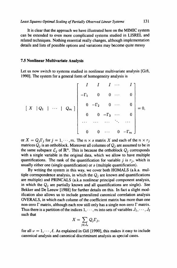
Let us now switch to systems studied in nonlinear multivariate analysis [Gifi, 1990]. The system for a general form of homogeneity analysis is

I I I I

0 0 0

[ X I Ql I ' · · I Qm ] =0, 0 0

o o -ra o

or X = Qiri for j = 1, · · ·, m. Then x s matrix X and each of then x ri matrices Qi is an orthoblock. Moreover all columns of Qi are assumed to be in the same subspace C; of Rn. This is because the orthoblock Qi corresponds with a single variable in the original data, which we allow to have multiple quantifications. The rank of the quantification for variable j is ri, which is usually either one (single quantification) or s (multiple quantification).

By writing the system in this way, we cover both HOMALS (a.k.a. mul­tiple correspondence analysis, in which the Qi are known and quantifications are multiple) and PRINCALS (a.k.a nonlinear principal component analysis, in which the Qi are partially known and all quantifications are single). See Bekker and De Leeuw [1988] for further details on this. In fact a slight mod­ification also allows us to include generalized canonical correlation analysis OVERALS, in which each column of the coefficient matrix has more than one non-zero r matrix, although each row still only has a single non-zero r matrix. Thus there is a partition of the indices 1, · · · , m into sets of variables J1, · · · , lt such that

X= L:: Q;r;, jEJ11

for allv = 1, · · ·, l. As explained in Gifi [1990], this makes it easy to include canonical analysis and canonical discriminant analysis as special cases.

132 JanDe Leeuw

The actual majorization algorithm from OVERALS is implemented in R by DeLeeuw and Ouwehand [2003]. The implementation has one additional feature, to deal with ordinal variables in the case of multiple quantifications. We can require Qi to be an orthoblock, with all its columns in the subspace Lj, but with, in addition, its first column in a cone ICj U Lj. Thus we can re­quire the leading quantification of a variable to be ordinal, while the remaining quantifications are orthogonal to the leading one.

If all variables are single, then homogeneity analysis becomes principal component analysis. Combining this with the ideas from the previous section show how explicit orthoblocks or errors can be introduced into the technique, so that we obtain versions of factor analysis or canonical analysis with orthog­onal error.

References

Bekker, P., & DeLeeuw, J. (1988). Relation between variants of nonlinear principal component analysis. In J.L.A. Van Rijckevorsel & J. De Leeuw (Eds.), Component and correspondence analysis. Chichester: Wiley.

Breiman, L., & Friedman, J.H. (1985). Estimating optimal transformations for multiple regression and correlation. Journal of the American Sta­tistical Association, 80, 580-619.

DeLeeuw, J. (1988). Multivariate analysis with linearizable regressions. Psy­chometrika, 53, 437-454.

DeLeeuw, J. (1990). Multivariate analysis with optimal scaling. In S. Das Gupta & J. Sethuraman (Eds.), Progress in multivariate analysis. Cal­cutta: Indian Statistical Institute.

DeLeeuw, J. (1993). Some generalizations of correspondence analysis. In C.M. Cuadras & C.R. Rao (Eds.), Multivariate analysis: Future di­rections 2. Amsterdam: North-Holland.

DeLeeuw, J. (1994). Block relaxation methods in statistics. In H.H. Bock, W.

Lenski & M.M. Richter (Eds.), Jnfonnation systems and data analy­sis. Berlin: Springer.

DeLeeuw, J., & Michailidis, G. (1999). Block relaxation algorithms in statis­tics. http://www.stat.ucla.edu/deleeuw/block.pdf.

DeLeeuw, J., & Michailidis, G., & Wang, D.Y. (1999). Correspondence anal­ysis techniques. In S. Gosh (Ed.), Multivariate analysis, design of experiments, and survey sampling. New York: Marcel Dekker.

DeLeeuw, J. & Ouwehand, A. (2003). Homogeneity analysis in R (Technical Report, UCLA Statistics). Los Angeles: UCLA Statistics Depart­ment.

Least Squares Optimal Scaling of Panially Observed Linear Systems 133

Gifi, A. (1990). Nonlinear multivariate analysis. Chichester: Wiley. Heiser, W. (1995). Convergent computing by iterative majorization: Theory

and applications in multidimensional data analysis. In W.J. Krzanowski (Ed.), Recent advantages in descriptive multivariate anal­ysis. Oxford: Clarendon.

Hom, R.A., & Johnson, C.R. (1991). Topics in matrix analysis. Cambridge: Cambridge University Press.

Joreskog, K.G. (1962). On the statistical treatment of residuals in factor anal­ysis. Psychometrika, 27, 335-354.

Joreskog, K.G., & Goldberger, A.S. (1975). Estimation of a model with multi­ple indicators and multiple causes of a single latent variable. Journal of the American Statistical Association, 70, 631-639.

Kiers, H.A.L., Takane, Y., & Mooijaart, A. (1993). A monotonically conver­gent algorithm for FACTALS. Psychometrika, 58, 567-57 4.

Koyak, R. (1987). On measuring internal dependence in a set of random vari­ables. Annals of Statistics, 15, 1215-1228.

Lange, K., Hunter, D., & Yang, I. (2000). Optimization transfer using surro­gate objective functions (with discussion). Journal of Computational and Graphical Statistics, 9, 1-59.

Meulman, J.J. & Heiser, W.J. (1999). SPSS Categories 10.0. Chicago: SPSS. Michailidis, G., & DeLeeuw, J. (1999). The Gifi system for descriptive mul­

tivariate analysis. Statistical Science, 13, 307-336. Mooijaart, A. (1984). The nonconvergence of FACTALS: A nonmetric com­

mon factor analysis. Psychometrika, 49, 143-145. Nevels, K. ( 1989). An improved solution for FACTALS: a nonmetric common

factor analysis. Psychometrika, 54, 339-343. Reinsel, G.C., & Velu, R.P. (1998). Multivariate reduced-rank regression (Lec­

ture notes in statistcs No. 136). Berlin: Springer. SAS. (1992). SAS!STAT software: Changes and enhancements (Technical re­

port P-229). Cary NC: SAS Institute. Takane, Y., Young, F.W., & DeLeeuw, J. (1979). Nonmetric common factor

analysis: An alternating least squares method with optimal scaling. Behaviormetrika, 6, 45-56.

Whittle, P. On principle components and least squares methods in factor anal­ysis. Skandinavisk Aktuarietidskrift, 35, 223-239.

Young, F.W. (1981). Quantitative analysis of qualitative data. Psychometrika, 46, 357-388.

Young, G. (1940). Maximum likelihood estimation and factor analysis. Psy­chometrika, 6, 49-53.

Zangwill, W.I. (1969). Nonlinear programming: A unified approach. Engle­wood-Cliffs NJ: Prentice-Hall.

134 JanDe Leeuw

Appendix. Augmented Procrustus

Suppose X is ann x m matrix of rank r. Consider the problem of maximizing tr U' X over then x m matrices U satisfying U'U =I. This is known as the Procrustus problem, and it is usually studied for the case n 2: m = r. We want to generalize ton 2: m 2: r. For this, we use the singular value decomposition

X= [ Kt nxr [

A K rxr

nx(n°-r) ] 0

(n-r)xr

0 rx(m-r)

0 (n-r)x(m-r)

Theorem 1 The maximum ojtr U' X overn x m matrices U satisfying U'U = I is tr A, and it isattainedforany U of the form U = K1 L~ + K 0 VL0, where Vis any (n- r) x (m- r) matrix satisfying V'V =I.

ProofVsing a symmetric matrix of Lagrange multipliers leads to the stationary equations X = UM, which implies X'X = M 2 or M = ±(X'X)112. It also implies that at a solution of the stationary equations tr U' X = ±tr A. The negative sign corresponds with the minimum, the positive sign with the maximum.

Now

l [ M = [ ::~r Lo mx(m-r)

If we write U in the form

U = [ Kt nxr

A rxr

0 (m-r)xr

Ko nx(n-r)

0 rx(m-r)

ll 0 (m-r)x(m-r)

u. l rxm

Uo (n-r)xm

then X = U M can be simplified to

UILI =I,

UoL1 = 0,

L'

l I

rxm

L' 0 (m-r)xm

with in addition, of course, U{ U1 + U0U0 = I. It follows that U1 = L~ and

u0 v L0 = ' (n- r) x m (n- r) x (m- r) (m- r) x m

with V'V = I. Thus U = K 1 L~ + K 0 V L0.