CHAPTER 7 HEAVY UTY - Pages...• Trip Assignment. The model incorporates a multiclass assignment...

CHAPTER 7 - HEAVY DUTY TRUCK MODEL

Contents Introduction ....................................................................................................... 7-1 HDT Model Structure ..................................................................................... 7-1 Internal HDT Model ........................................................................................ 7-3 External HDT Model ....................................................................................... 7-8 Port HDT Model ........................................................................................... 7-10 Intermodal HDT Trips ................................................................................. 7-14 HDT Time of Day Factoring & Assignment ............................................ 7-16

SCAG 2008 Regional Model

1


CHAPTER 7 – HEAVY DUTY TRUCK MODEL Introduction As part of the Regional Model Update, SCAG commissioned a team to develop improvements and enhancements to the Heavy Duty Truck (HDT) Model. This Chapter provides the technical approach used to implement various model improvements. A key element of this model development effort was the collection and analysis of HDT trip data. A report documenting this data collection effort is available from SCAG2 This Chapter addresses the various elements of the Heavy Duty Truck Model, including internal and external HDT trips, Port HDT trips and Intermodal HDT trips. HDT Model Structure Figure 7-1 provides a flow chart of the overall structure of the HDT model. The model forecasts trips for three HDT weight classes: light-heavy (8,500 to 14,000 lbs. gross vehicle weight (GVW); medium-heavy (14,001 to 33,000 lbs. GVW); and heavy-heavy (>33,000 lbs. GVW). The key components of the new HDT Model are the following: • External Trip Generation and Distribution Model. This component estimates the trip table for

all interregional truck trips based on commodity flow patterns that link Southern California with the rest of the nation. The previous model used a commodity flow database obtained from outside sources, and included procedures for converting annual tonnage flows at the county level to daily truck trips at the TAZ level. The updated model replaces the older Caltrans Intermodal Transportation Management System (ITMS) commodity flow database with a new TRANSEARCH database from IHS/Global Insight. Adjustments were made to the TransCAD scripts that convert annual tonnage flows into daily truck trip tables. These modifications are a result of differences in data formats between TRANSEARCH and ITMS.

• Internal Trip Generation and Distribution Models. This component of the HDT Model estimates

trip tables for intraregional trips. Trip generation is based on trip rates (number of trips per employee or household) for different land uses/industry sectors at the trip ends. This basic structure was retained, although all of the current trip rates were updated with new survey data. Other trip generation specifications (e.g., trip rates as a function of size of firm or more detailed industry/land use classifications) were reviewed, but it was determined that these specifications were not supported by currently available forecast data from SCAG.

The trip distribution process was modified by developing a matrix of factors that indicate the trip interchange relationships among different land use types (i.e., what fraction of trips originating at a land use such as manufacturing sites go to warehouses vs. other manufacturing sites, etc.). The GPS survey data was used to develop a series of gravity models for each truck class. This offers some of the benefits of tour-based models by directing trips from zone to zone based on logical relationships amongst land use types without the extensive data requirements (typically difficult to collect from trip diary surveys) that are required to support development of a full tour-based model.

2 Cambridge Systematics, Inc., SCAG Task 4 Data Verification and Analysis – Final Report, October 2010.

2


Figure 7-1: Final HDT Model Structure

Trip Generation

Production and Attraction Table for 8 LU, 3 GVW

Composite Cost Trip Distribution and Apply TOD

Factors

Time & Distance Skims

Truck Cost per Mile Including

Fuel

8 x 8 LU Interchange

Matrix

Daily I-I Trip Tables for 3 GVW

and 4 TOD Periods

TOD Factors

Socio-economic

External Truck Model

External Station

Analysis

Year

Socio-economic

Transearch

Data

Daily IE-EI-EE Truck Trip Table for 3 Truck Sizes

and for each TOD period

TOD Factors

Combine Truck Tables by TOD

Periods

Port Tables by TOD (From QuickTrips)

IMX Tables by TOD (Exogenous Input)

Traffic Assignment

Loaded Network

Truck Trip Tables by TOD Periods for 3

GVW

Auto Trip Tables by TOD Periods

Truck

Input File

Input Parameter

Program

Output File


Page 7-3

• Special Generator Trip Generation and Distribution Models. These models include the port model and the intermodal rail model. All of the input parameters to the port trip generation model were updated to reflect current port capacity improvements and throughput forecasts. This model update also implements a procedure to incorporate secondary port truck trips. These are cargo trips from intermediate handling locations (container staging areas, transshipment sites, etc.) to final destinations. Additionally there are secondary (empty) movements of trucks associated with port truck trips, for purposes of truck repositioning. Both cargo and empty truck secondary trips are allocated to other destination in the regions using the gravity model distribution.

• Trip Assignment. The model incorporates a multiclass assignment combining the truck trip tables

with the passenger trip tables. Prior to assignment, the truck trip tables are converted to PCEs. The PCE factors were adapted from the TRB Highway Capacity Manual3, and are a function of the percent truck volume and length and steepness of grades. Five time periods are used to assign truck trips, consistent with the auto trip assignment. Updated time-of-day factors were developed using data from permanent classification count stations, weigh-in-motion (WIM), and vehicle classification counts.

Internal HDT Model Internal HDT Trip Generation Model The internal truck trip generation model is land use-based, where trip rates are multiplied by employment by industry sector to obtain internal truck trip productions and attractions. All the internal truck travel in the region is associated with eight broad but distinct land uses, namely, households, agriculture/mining/construction, retail, government, manufacturing, transportation/utility, wholesale, and other (service). The trip rates (i.e., truck trips per employee) for every land use were updated based on recent data collection efforts –establishment surveys and third-party truck GPS data. Land Use and Socioeconomic Data The socioeconomic data used by the Internal HDT Model is consistent with those data used by the passenger model, except that the employment data are stratified into more employment categories. The 22 two-digit NAICS categories of employment were mapped to 10 final categories to account for truck trip generation similarities. This employment category mapping is shown in Table 7-1. These stratified employment types, plus households, support eight land use purposes for the HDT trip generation models: Households, Agriculture/Mining/Construction, Retail, Governments, Manufacturing, Transportation and Utility, Wholesale, and Other (service).

3 Highway Capacity Manual. Volume 2: Uninterrupted Flow. Transportation Research Board: Washington D.C., 2010.


Page 7-4

Table 7-1: Aggregated Two-Digit NAICS Categories

Two-Digit Two-Digit Description Aggregate Categories for Trip Generation Models

1 11 Agriculture, Forestry, Fishing, and Hunting 1 Agriculture, Forestry, Fishing, and Hunting

2 21 Mining 2 Mining 3 22 Utilities 3 Utilities 4 23 Construction 4 Construction 5 31 Manufacturing 5 Manufacturing 6 42 Wholesale Trade 6 Wholesale Trade 7 44 Retail Trade 7 Retail Trade 8 45 Retail Trade 7 Retail Trade 9 48 Transportation and Warehousing 8 Transportation and Warehousing 10 49 Transportation and Warehousing 8 Transportation and Warehousing 11 51 Information Services 9 FIRES 12 52 Finance and Insurance 9 FIRES 13 53 Real Estates, and Rental and Leasing 9 FIRES 14 54 Professional, Scientific, and Technical Services 9 FIRES 15 55 Management of Companies and Enterprises 9 FIRES

16 56 Administrative and Support, and Waste Management and Remediation Services 9 FIRES

17 61 Educational Services 10 EDU 18 62 Health Care, and Social Assistance 9 FIRES 19 71 Arts, Entertainment, and Recreation 9 FIRES 20 72 Accommodation, and Food Services 9 FIRES

21 81 Other Services (Except Public Administration) 9 FIRES

22 92 Public Administration 11 GOVT Internal HDT Trip Rates Trip rates derived from establishment surveys and GPS data for each truck type and land use are shown in Table 7-2.

Table 7-2: Internal HDT Trip Rates

Category Light HDT Trip Rate

Medium HDT Trip Rate

Heavy HDT Trip Rate

Households 0.0147 0.0046 0.0072 Agriculture/Mining/Construction 0.0804 0.0778 0.0715 Retail 0.0663 0.0662 0.0703 Government 0.0296 0.0150 0.0148 Manufacturing 0.0613 0.0655 0.0924 Transportation/Utility/Warehousing 0.1583 0.1819 0.3206 Wholesale 0.0916 0.0968 0.1316 Other (Service) 0.0095 0.0111 0.0151

-5


Table 7-3 shows the 2008 HDT trip generation estimates. As expected, households in the region generate a high number of trip ends. This is mostly due to the fact that land uses such as transportation and warehousing, utilities, service and retail deliver goods and provide services to residential neighborhoods. The largest HDT trip generator is the transportation and utility land use that includes trucks involved in power generation, water supply and sewage treatment, all kinds of transportation (trucking industry, taxi, and chartered services), and postal and courier services. The second highest generators of HDT trips are retail and manufacturing land uses, which account for a major share of employment in the region and serve the vast area and population of the six-county SCAG region.

Table 7-3: 2008 Internal HDT Trip Generation Estimates

Land Use Light HDT Trip Ends

Medium HDT Trip

Ends

Heavy HDT Trip Ends

Total Trip Ends

Percent of Total Trip

Ends Households 85,194 26,692 42,031 153,917 15% Ag/Mining/Construction 39,080 37,833 34,784 111,698 11% Retail 55,607 55,527 58,953 170,087 17% Governments 7,339 3,733 3,670 14,742 1% Manufacturing 46,715 49,902 70,471 167,087 17% Transportation/Utility/Warehousing 57,057 65,584 115,586 238,227 24%

Wholesale 36,468 38,549 52,395 127,412 13% Other 2,937 3,422 4,664 11,023 1% Total 330,398 281,242 382,553 994,194 Internal HDT Trip Distribution Model The trip distribution process was modified by developing a matrix of factors that indicate the trip interchange relationships among different land use types (i.e., what fraction of trips originating at a land use such as manufacturing sites go to warehouses vs. other manufacturing sites, etc.). The internal HDT trip distribution model uses a gravity formulation, stratified by land use type at both the production and the attraction end of the trip. This results in a total of 64 gravity models for each truck type (LHDT, MHDT and HHDT). After trip distribution, the 64 different trip matrices are combined into a single matrix for each truck type, so that only three matrices are passed on to time-of-day factoring and trip assignment. Truck trips are distributed using composite cost impedances that accounts for time and distance-based monetary costs in addition to travel time. Based on a review of the literature, the appropriate distance-based costs for the SCAG model are identified in a report commissioned by the Minnesota DOT4. These costs account for fuel, tires, maintenance and repair, and depreciation. The link composite cost is calculated as shown in the equation below. The corresponding unit costs are shown in Table 7-4. Composite Cost = Cost per hour * Congested time +

[Fuel Price / Fuel efficiency + Cost per mile (excluding fuel)] * Distance 4 Levinson, David Matthew, Corbett, Michael J. and Hashami, Maryam, Operating Costs for Trucks, (2005) http://papers.ssrn.com/sol3/Delivery.cfm/SSRN_ID1736159_code807532.pdf?abstractid=1736159&mirid=1.


Page 7-6

Table 7-4: Composite Truck Unit Costs

Truck Type Cost per Hour Fuel Efficiency (MPG)

Cost per Mile (excluding

fuel) Fuel Price per Gallon

LHDT $13.84 8.5 $0.14 $3.13 (a)

MHDT $19.21 7.0 $0.23 $3.15 (b)

HHDT $19.21 6.0 $0.26 $3.15 (b)

(a) Assumes a fleet mix of 60% gasoline and 50% diesel powered trucks. (b) Average price of diesel fuel in California between 2006 and 2011.

The GPS survey of truck trips provided the data to calibrate the model friction factors. These data were used to build observed truck trip flow matrices, stratified by truck type (LHDT, MHDT and HHDT). The TransCAD gravity model calibration utility was used to calibrate the fraction factors that best matched the observed truck flow matrices, given the composite cost impedances and land-use based trip productions and attractions. Figures 7-2 to 7-4 show the trip length calibration, respectively for each truck class.

Figure 7-2 LHDT Internal Truck Trip Length Calibration

0%

5%

10%

15%

20%

25%

30%

35%

0 50 100 150 200 250

% o

f LH

DT

Tri

ps

Travel Time (minutes)

LHDT 2008 Model

LHDT 2007 Trip Diary

Trimble GPS Data

LHDT Coincidence: 0.74

7


Figure 7-3 MHDT Internal Truck Trip Length Calibration

Figure 7-4 HHDT Internal Truck Trip Length Calibration

0%

5%

10%

15%

20%

25%

30%

35%

0 50 100 150 200 250

% o

f MH

DT

Tri

ps


LHDT 2008 Model

MHDT 2007 Trip Diary

Trimble GPS Data

0%

2%

4%

6%

8%

10%

12%

14%

16%

18%

0 50 100 150 200 250

% o

f HH

DT

Tri

ps


HHDT 2008 Model

HHDT 2007 Trip Diary

ATRI GPS Data

HHDT Coincidence: 0.74

MHDT 2008 Model

MHDT Coincidence: 0.73


Page 7-8

External HDT Model The external HDT Model consists of internal-external & external-internal trips (IE/EI), and external-external truck trips (EE). The IE/EI HDT trips are generated and distributed using a combination of commodity flow data at the county level and 2-digit NAICS employment data for allocating county data to TAZs. Growth factors developed using the commodity flow data at a county level and external cordon are used to forecast future year external HDT trips from the base year trip flow matrices. The external HDT Model is based on the 2007 TRANSEARCH commodity flow table. The TRANSEARCH data are provided as annual flows in tons and are converted to daily weekday flows using an annualization factor of 306 (6 days per week for 51 weeks) for all commodities. The flows are converted from tons to trucks using the payload factors shown in Table 7-5. These payload factors were developed using data from the 2002 Vehicle Inventory and Use Survey (VIUS). The methodology that converts commodity flows to annual HDT trips at the TAZ level is described below for various direction, commodity and shipment type combinations. Outbound Truck Load and Private Carrier Shipments The external trip end of the outbound commodity flows are allocated to external cordon stations using survey data from the SCAG region. The internal trip end of the outbound commodity flows is disaggregated from counties to TAZs based on shares of employment in the manufacturing, agricultural, mining industries, or warehousing land use acreage, depending on the type of commodity. Inbound Truck Load and Private Carrier Shipments The external trip end of the inbound commodity flows are allocated to cordon stations as described above for outbound flows. To establish the internal TAZ trip end, flows of each commodity destined to warehouses are estimated using Reebie data, and then disaggregated to TAZs based on the share of warehousing land use acreage. The remaining non-warehouse destination flows are assumed to be destined directly to manufacturing facilities. To disaggregate these flows, the fraction of each commodity consumed by different industries is determined using an Input-Output table, and then disaggregated to TAZs based on shares of employment in the corresponding industry.

Less than Truck Load (TL) Shipments SCAG inbound and outbound LTL shipments typically move through LTL terminals at the origin and destination so the same methodology is used for both directions. Also, since LTL shipments could carry any commodity, the approach is the same for all commodities. Truck load payload factors are used because payloads for LTL shipments cannot be determined (each LTL shipment carries many commodities with varying payloads). The external trip end of the LTL commodity flow is allocated to cordon stations as described above for truck load shipments. The internal trip end is disaggregated from county to TAZ based on the share of LTL trucking employment.

9


Table 7-5: External HDT Commodity Payload Factors

Commodity Payload Factors (Tons per Truck)

STCC Description LHDT MHDT HHDT

1 Farm Products 1 2 16 8 Forest Products 3 6 14 9 Fresh Fish or Other Marine Products 2 2 10

10 Metallic Ores 3 3 24 11 Coal 3 3 18 13 Crude Petroleum, Natural Gas, or Gasoline 3 6 15 14 Non-metallic Minerals 4 5 16 19 Ordinance or Accessories 2 5 14 20 Food or Kindred Products 3 4 15 21 Tobacco Products, excluding Insecticides 3 6 15 22 Textile Mill Products 1 4 11 23 Apparel or Other Finished Textile Products 5 6 9 24 Lumber or Wood Products, excluding Furniture 4 6 16 25 Furniture or Fixtures 2 3 9 26 Pulp, Paper, or Allied Products 2 7 13 27 Printed Matter 2 7 15 28 Chemicals or Allied Products 2 5 14 29 Petroleum or Coal Products 3 6 11 30 Rubber or Miscellaneous Plastics Products 3 5 12 31 Leather or Leather Products 3 6 13 32 Clay, Concrete, Glass, or Stone Products 3 7 14 33 Primary Metal Products 5 6 15 34 Fabricated Metal Products 5 5 11 35 Machinery, excluding Electrical 2 3 9 36 Electrical Machinery, Equipment, or Supplies 2 5 8 37 Transportation Equipment 2 7 11 38 Instruments, Photographic Goods, Optical Goods, Watches, or Clocks 2 4 10 39 Miscellaneous Products of Manufacturing 2 6 8 40 Waste or Scrap Materials 2 3 14 43 Mail 3 4 14 44 Freight Forwarder Traffic 3 1 7 45 Shipper Association or Similar Traffic 3 6 9 46 Freight All Kinds 3 5 12 47 Small Packages, LTC or LTL 3 6 10 48 Waste Hazardous Materials or Waste Hazardous Substances 3 6 15


Page 7-10

External – External HDT Trips The 2007 TRANSEARCH data identify EE truck freight flows passing through the SCAG region. To assign the cordon station to each EE trip end, a method similar to the one used for the external end of the IE/EI trips was used. Empty Truck Trips To account for all external truck trips in the SCAG region, empty truck are added to the loaded truck trips estimated from the commodity flows. Empty truck trip percentages at each external cordon location were generated from survey data. Assuming the empty truck fractions to be the same for all O-D pairs for an external cordon, empty truck trips are added to the loaded truck trips between SCAG TAZs and external TAZs. Port HDT Model Ports TAZ Development The SCAG Tier 1 Zone System consists of 4,192 TAZs, including 40 TAZs that represent the Ports areas. The Port HDT Model was updated to use a more refined set of port TAZs, developed by the Port of Long Beach. This zone system, called Port TAM, includes a total of 85 Ports area TAZs, for a total of 4,251 Tier 1 TAZs. Table 7-6 below provides a summary breakdown of the 4,251 TAZ system.

Table 7-6: Port TAM 4,251 TAZ System

from Zone ID To Zone ID Zone Type Total

1 4109 Internal zones 4,109

4110 4149 External zones 40

4150 4161 Airport zones 12

4162 4246 Port zones 85

4247 4251 Extra zones 5

Total Zones

4,251 Terminal Gate Surveys Origin-destination (OD) truck surveys were conducted in early 2010 at the Ports of Los Angeles and Long Beach Marine Terminals. The marine terminals are distribution points where international cargo is loaded onto trucks and rail. The survey was conducted to obtain OD pattern information by truck type. Surveys were conducted at six Port of Long Beach terminals (ITS, PCT, LBCT, CUT, SSA, and HANJIN) and six Port of Los Angeles terminals (YTI, MAERSK, EVERGREEN, TRAPAC, YANG MING, and APL). A total of 23,030 survey sheets were distributed and 3,559 were returned. From the returned surveys, 2,981 origin trips were fully completed and geo-coded, and another 2,593 destination trips were also

11


fully completed and geo-coded for a total of 5,574 trips. Tables 7-7 and 7-8 present the survey sample origins and destinations by container type. The marine terminal truck trips exhibited the following OD patterns:

• 12% traveled to the Ports areas & nearby locations • 30% traveled to Gateway cities locations • 20% traveled to off-dock yards • 33% traveled to locations within the rest of the SCAG region • Less than 5% traveled to out of state locations • 98% of the off-dock intermodal yard traffic went to the four main intermodal yards (ICTF,

Hobart, East LA, and LATC). Almost no traffic was recorded from yards at Industry and San Bernardino.

Table 7-7: Survey Sample Origins

Terminal Bobtails Chassis Containers Total

ITS 121 45 259 425 PCT 98 33 215 346 LBCT 165 14 282 461 CUT 94 45 151 290 SSA 75 26 73 174 HANJIN 142 13 198 353 YTI 9 3 21 33 MAERSK 107 31 80 218 EVERGREEN 59 21 104 184 TRAPAC 163 13 166 342 YANG MING 48 10 69 127 APL 13 1 14 28 Total 1,094 255 1,632 2,981

Table 7-8: Survey Sample Destinations

Terminal Bobtails Chassis Containers Total ITS 116 22 246 384 PCT 77 22 173 272 LBCT 115 15 258 388 CUT 89 18 141 248 SSA 30 14 94 138 HANJIN 85 31 187 303 YTI 15 1 16 32 MAERSK 35 31 140 206 EVERGREEN 55 6 103 164 TRAPAC 86 14 213 313 YANG MING 23 10 81 114 APL 10 3 18 31 Total 736 187 1670 2,593


Page 7-12

Port Truck Trip Generation The port trip generation model was developed in 2008 based on a detailed port area zone system and specialized trip generation rates for autos and trucks by type (Bobtail, Chassis, and Containers). Port truck trip generation has two components: 1) container terminal truck trips, and 2) non-container terminal truck trips. Container Terminal Truck Trip Generation The container terminal truck trip generation model for the ports is referred to as the QuickTrip Model. QuickTrip was originally developed for the Ports of Los Angeles and Long Beach. The Model includes detailed input variables such as mode split (rail versus truck moves), time-of-day factoring, weekend moves, empty return factors, and other characteristics that affect the number of trucks entering and exiting through the terminal gates. The relevant input data for each container terminal include the following:

• Peak monthly Twenty-Foot Equivalent Units (TEU) throughput. • TEU-to-lift conversion factor: factor determining the average number of TEUs associated with

each lift at the terminal. • TEU land-side throughput distributions: percent of TEU throughput associated with on-dock

intermodal imports, on-dock intermodal exports, off-dock intermodal imports, off-dock intermodal exports, local imports, local exports, empties, and trans-shipments across the wharf.

• Number of operating days during the week. • Percent of throughput moved during each terminal operating shift (for the day, second and hoot

shifts). QuickTrip produces the following truck trip outputs for each terminal:

• Monthly gate transactions • Peak week truck trip volume • Daily truck trips, and truck trips by each hour of the day by type of truck trip (bobtail, chassis,

container, empty), and direction (arrival at and departure from the terminal) QuickTrip can be used to generate base as well as future year truck trips by truck type and direction for each terminal, using the model inputs described earlier for each specific year. The inputs that are particularly expected to change for different years include the peak monthly TEU throughput, and the TEU land-side throughput distributions (based on expected increase in on-dock intermodal capacity at the port terminals in the future). Additionally, the model has the capability to analyze the impacts of other port truck trip reduction strategies such as virtual container yards and off-peak truck diversions, using specific inputs associated with these strategies. The Model was enhanced to allow the user to assess whether the estimated capacity of each rail yard has been exceeded. If so, traffic is iteratively re-allocated to other yards that are not over capacity. The enhanced model also allows the user to choose different efficiency factors, such as “percent double cycle trucks,” for different off-dock yards. In the original version, the user had to use the same variables for the entire off-dock market.

13


Non-Container Terminal Truck Trip Generation

Non-container terminal truck trip generation estimates were also developed for the Ports as part of the Port truck trip generation process. This includes trips to and from all of the other types of marine terminals (automobile terminals, dry bulk terminals, liquid bulk terminals and break-bulk terminals). In addition, there are many non-terminal land uses located throughout the ports (e.g., administrative offices, recreation, commercial, government buildings) that potentially generate truck traffic. Existing non-container terminal truck trips were developed by conducting a series of driveway and midblock truck counts throughout the Ports. A number of specific terminals were counted at their driveways, while other terminals and miscellaneous land use activities were reflected via the use of downstream roadway truck counts. In some cases, a roadway truck count was used to represent the trip generation of a group of non-container terminals and other land uses. Port Trip Table Distribution The zone to zone distribution of port truck trips is based on a fixed OD matrix. A detailed and comprehensive truck driver survey was undertaken by the ports at the marine container terminals. The survey was used to develop detailed origin-destination “trip tables” for use in the Port area travel demand model. The stated trip OD from every valid survey was correlated with the travel demand model TAZ system. The survey results were then used to develop port truck OD matrices by truck type for use in the model. Distribution patterns were developed separately for arrival trips and departure trips for each terminal. A total of 15 Port Truck Trip Tables were developed (5 time periods by 3 vehicle classes): AM, MD, PM, EV and NT time periods, and Bobtails, Chassis and Container truck trips. The time periods are consistent with those used by the passenger model. Empty container and loaded container truck types are combined into one truck type called container truck type. For terminals with few or no observations (Pier C, YTI and APL) an average distribution of all surveyed records was used. Before creating survey frequency distribution vectors, survey sample trips were adjusted to exclude trips that have both OD within the same terminal.

Base Year Port Trip Tables Summary Summaries of 2008 Port truck trips are shown in Tables 7-9 and 7-10.

Table 7-9: 2008 Port HDT Trips by Truck Type

Time Period Bobtails Chassis Containers Total

AM 1,339 415 1,858 3,612

MD 7,756 2,439 11,037 21,232

PM 3,669 1,159 5,248 10,076

EV 1,888 596 2,696 5,180

NT 2,832 895 4,045 7,772 Daily 17,484 5,504 24,884 47,872


Page 7-14

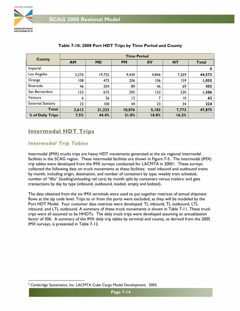
Table 7-10: 2008 Port HDT Trips by Time Period and County

County Time Period

AM MD PM EV NT Total Imperial

0

Los Angeles 3,276 19,752 9,430 4,846 7,269 44,573 Orange 108 475 206 106 159 1,055 Riverside 46 204 89 46 69 455 San Bernardino 153 675 295 153 230 1,506 Ventura 6 26 12 7 10 62 External Stations 23 100 44 23 34 224

Total 3,612 21,233 10,076 5,182 7,772 47,875 % of Daily Trips 7.5% 44.4% 21.0% 10.8% 16.2% Intermodal HDT Trips Intermodal Trip Tables Intermodal (IMX) trucks trips are heavy HDT movements generated at the six regional intermodal facilities in the SCAG region. These intermodal facilities are shown in Figure 7-5. The intermodal (IMX) trip tables were developed from the IMX surveys conducted for LACMTA in 20055. These surveys collected the following data on truck movements at these facilities: total inbound and outbound trains by month, including origin, destination, and number of containers by type; weekly train schedule; number of “lifts” (loading/unloading rail cars) by month split by containers versus trailers; and gate transactions by day by type (inbound, outbound, loaded, empty and bobtail).

The data obtained from the six IMX terminals were used to put together matrices of annual shipment flows at the zip code level. Trips to or from the ports were excluded, as they will be modeled by the Port HDT Model. Four customer data matrices were developed: TL inbound, TL outbound, LTL inbound, and LTL outbound. A summary of these truck movements is shown in Table 7-11. These truck trips were all assumed to be HHDTs. The daily truck trips were developed assuming an annualization factor of 306. A summary of the IMX daily trip tables by terminal and county, as derived from the 2005 IMX surveys, is presented in Table 7-12.

5 Cambridge Systematics, Inc. LACMTA Cube Cargo Model Development. 2005.

15


Figure 7-5: Intermodal Facilities in the SCAG Region

Table 7-11: 2005 Domestic IMX (Non-Port) Annual Truck Trips

Domestic BNSF Hobart

BNSF San Bernardino

UP City of Industry

UP East LA

UP ICTF

UP LATC Total

Inbound 444,204 433,333 93,789 96,757 2,463 21,812 1,092,357 TL/IMC 273,495 300,654 81,789 85,567 2,276 18,781 762,562 LTL 170,708 132,679 12,000 11,190 187 3,031 329,795

Outbound 445,011 458,677 78,431 69,837 662 21,353 1,073,970 TL/IMC 280,997 331,201 66,901 59,086 482 18,441 757,108 LTL 164,014 127,476 11,530 10,751 180 2,912 316,862

Total 889,214 892,009 172,220 166,594 3,125 43,165 2,166,327 TL/IMC 554,492 631,855 148,690 144,653 2,758 37,222 1,519,670 LTL 334,722 260,154 23,530 21,941 367 5,943 646,657

Table 7-12: 2008 Intermodal HHDT Trips by Terminal and County

IMX Terminal IMX

Terminal TAZ

Imperial Los Angeles Orange Riverside San

Bernardino Ventura Grand Total

Share by Terminal

UP ICTF 1,360 0 9 1 1 1 0 13 0% UP LATC 1,591 0 84 22 24 15 1 147 2% BNSF Hobart 1,679 10 1,722 280 327 532 36 2,905 40% UP East LA 1,702 2 322 110 78 73 4 589 8% UP City of Industry 2,304 6 283 152 112 49 3 606 8% BNSF San Bernardino 3,773 19 516 1,687 687 50 2 2,961 41%

Grand Total 37 2,937 2,252 1,228 720 47 7,221 Share by County 1% 41% 31% 17% 10% 1%


Page 7-16

Secondary HDT Trips The truck trip table calculated from the Port and IMX models comprises only the portion of the trip between those facilities and locations, primarily wholesale land uses, elsewhere in the SCAG region. These trips give rise to additional, “secondary” trips from these locations. That is, the first leg of this HDT trip chain is from Port or IMX to wholesale, while the second leg is from that wholesale land use to any internal TAZ in the six-county SCAG region. These trips should be represented as wholesale land use truck trips in the internal HDT Model. The Port and IMX implied secondary truck production and attractions were added to the internal trucks prior to trip distribution. Table 7-13 presents a summary of the total wholesale HHDT trips in the region that are computed from three models – internal HDT, Port and IMX.

Table 7-13: 2008 Wholesale HDT Trips

Truck Type/PA Internal HDT Port Model HHDT

IMX HHDT Trips

Total Wholesale

HHDT LHDT Productions 35,129

n/a LHDT Attractions 35,129 MHDT Productions 37,133 MHDT Attractions 37,133 HHDT Productions 50,470 12,885 3,405 66,760 HHDT Attractions 50,470 12,254 3,570 66,294

HDT Time-of-Day Factoring & Assignment The HDT Model uses fixed time-of-day factors derived from observed truck counts. The HDT time of time periods are consistent with the passenger model periods, namely:

• AM Peak: 6:00 AM – 9:00 AM • Mid-day: 9:00 AM - 3:00 PM • PM Peak: 3:00 PM - 7:00 PM • Evening: 7:00 PM – 9:00 PM • Night: 9:00 PM – 6:00 AM

The HDT diurnal factors were derived from the 2007 Vehicle Travel Information System (VTRIS)6 database. VTRIS is maintained by the FHWA Office of Highway Policy Information to track traffic trends, vehicle distributions and weight of vehicles to meet data needs specified in highway legislation. The VTRIS database contains truck classification counts spanning nearly half a year at many locations on SCAG interstate and state highways. The HDT time of day factors are shown in Table 7-14.

6 http://www.fhwa.dot.gov/ohim/ohimvtis.cfm

17


Table 7-14: HDT Time-of-Day Factors

Time Period Diurnal Factors

LHDT MHDT HHDT

AM Peak (6 AM - 9AM) 18.8% 18.0% 13.9% Midday (9 AM-3PM) 42.9% 46.5% 35.3% PM Peak (3 PM- 7PM) 20.3% 15.5% 16.7% Evening (7 PM - 9 PM) 4.8% 3.5% 7.2% Night (9 PM - 6AM) 13.2% 16.5% 26.9%

HDT trips are assigned simultaneously with the auto trips as part of a user equilibrium multiclass assignment. The assignment methodology is described in detail in Chapter 8 – Trip Assignment. Truck volumes are converted to PCEs following the procedures recommended in the 2010 Highway Capacity Manual. The PCE factors are a function of grade, length of the climb segment, and percent of truck volume, and vary by truck type (LHDT, MHDT and HHDT). These factors are shown in Table 7-15.

Table 7-15: HDT Passenger Car Equivalent Factors

Percent Trucks

Length of Grade in

miles

Light -Heavy Medium-Heavy Heavy-Heavy

% Grade % Grade % Grade

< 2 2 - 4 4 - 6 > 6 < 2 2 - 4 4 - 6 > 6 < 2 2 - 4 4 - 6 > 6

0-5%

< 1 1.3 1.5 3.0 4.0 1.5 2.0 3.5 5.0 2.5 2.5 4.5 6.0

1 - 2 1.3 2.5 4.0 5.0 1.5 3.5 5.0 6.5 2.5 5.0 7.5 12.5

> 1 1.3 2.5 4.0 5.0 1.5 3.5 5.0 6.5 2.5 5.0 7.5 12.5

5-10%

< 1 1.3 1.5 2.5 3.0 1.5 2.0 3.0 4.0 2.5 2.5 4.5 5.5

1 - 2 1.3 2.0 3.5 4.0 1.5 3.0 4.0 5.5 2.5 4.0 8.0 11.5

> 1 1.3 2.0 3.5 4.0 1.5 3.0 4.0 5.5 2.5 4.0 8.0 11.5

>10%

< 1 1.3 1.5 2.0 2.5 1.5 2.0 2.5 3.0 2.5 2.5 4.0 4.0

1 - 2 1.3 2.0 3.0 3.5 1.5 2.5 3.5 4.0 2.5 3.5 6.0 9.0

> 1 1.3 2.0 3.0 3.5 1.5 2.5 3.5 4.0 2.5 3.5 6.0 9.0

CHAPTER 7 HEAVY UTY - Pages...• Trip Assignment. The model incorporates a multiclass assignment...

Documents

Transcript of CHAPTER 7 HEAVY UTY - Pages...• Trip Assignment. The model incorporates a multiclass assignment...