Chapter 6: Viscous Flow in Ducts

058:0160 Chapter 6-part3

Professor Fred Stern Fall 2010 1

Chapter 6: Viscous Flow in Ducts

6.3 Turbulent Flow

Most flows in engineering are turbulent: flows over

vehicles (airplane, ship, train, car), internal flows (heating

and ventilation, turbo-machinery), and geophysical flows

(atmosphere, ocean).

V(x, t) and p(x, t) are random functions of space and time,

but statistically stationary flows such as steady and forced

or dominant frequency unsteady flows display coherent

features and are amendable to statistical analysis, i.e. time

and place (conditional) averaging. RMS and other low-

order statistical quantities can be modeled and used in

conjunction with the averaged equations for solving

practical engineering problems.

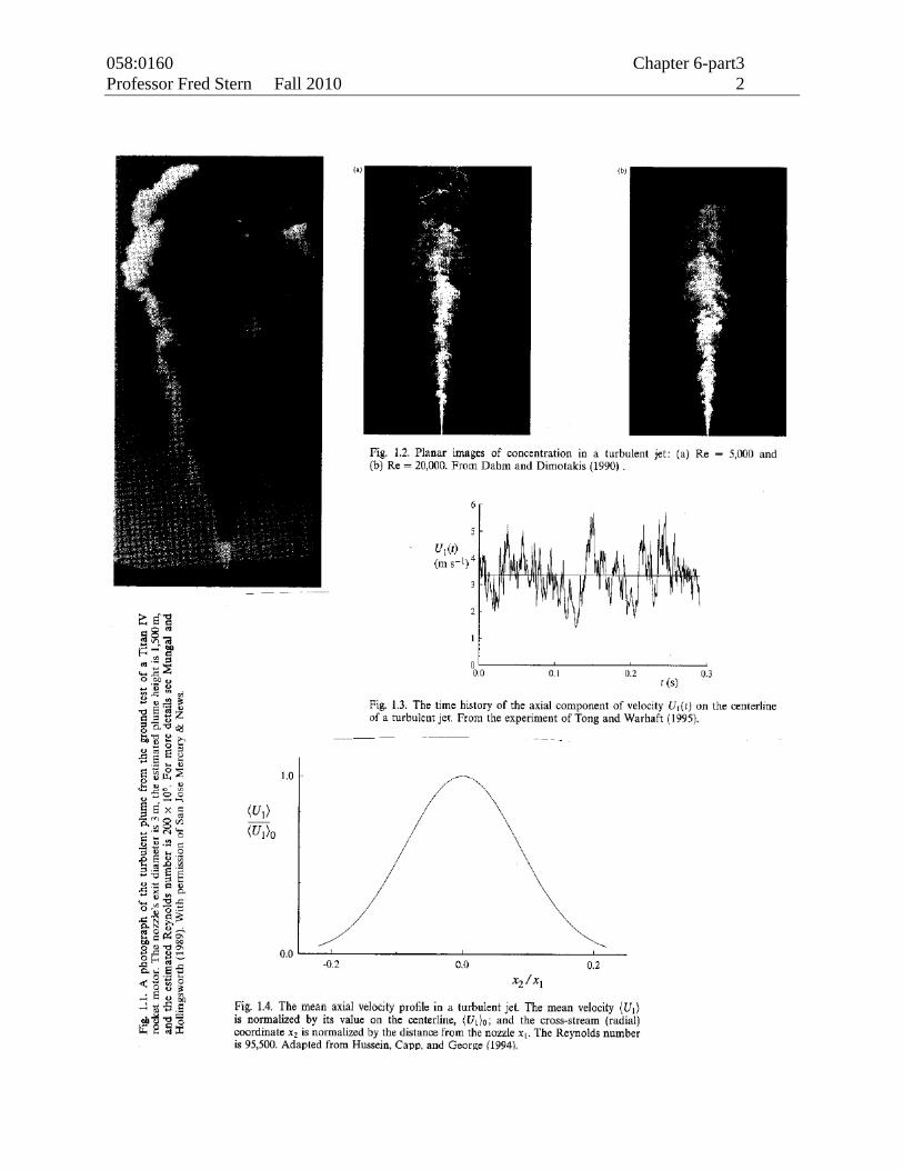
Turbulent motions range in size from the width in the

flow δ to much smaller scales, which become

progressively smaller as the Re = Uδ/υ increases.



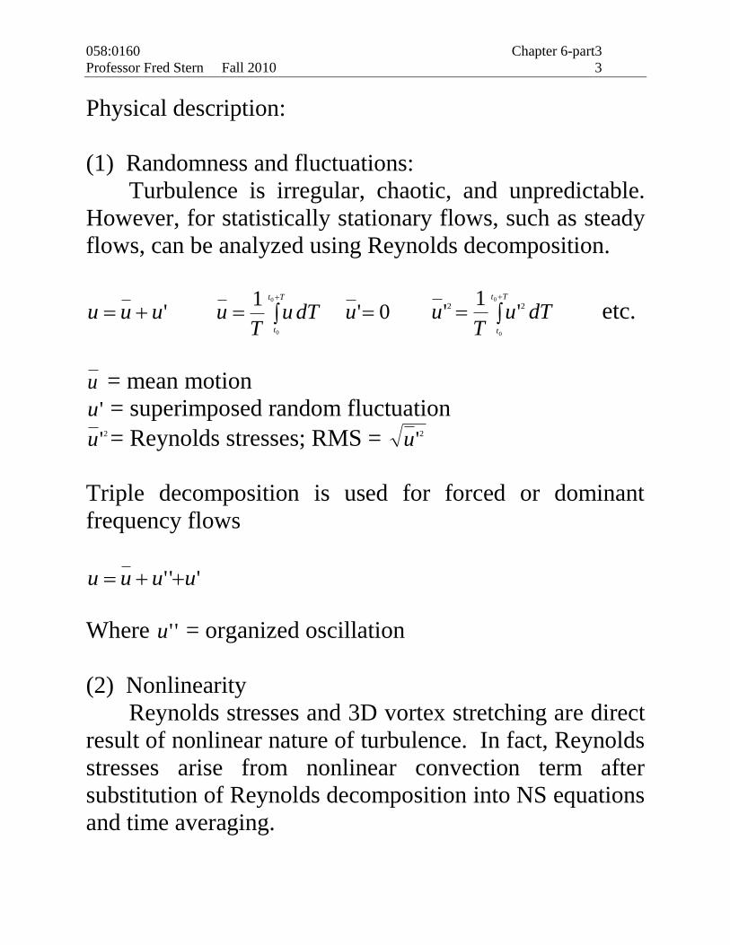
Physical description:

(1) Randomness and fluctuations:

Turbulence is irregular, chaotic, and unpredictable.

However, for statistically stationary flows, such as steady

flows, can be analyzed using Reynolds decomposition.

'uuu Tt

t

dTuT

u0

0

1 0'u dTu

Tu

Tt

t

0

0

22 '1

' etc.

u = mean motion

'u = superimposed random fluctuation 2'u = Reynolds stresses; RMS = 2'u

Triple decomposition is used for forced or dominant

frequency flows

''' uuuu

Where ''u = organized oscillation

(2) Nonlinearity

Reynolds stresses and 3D vortex stretching are direct

result of nonlinear nature of turbulence. In fact, Reynolds

stresses arise from nonlinear convection term after

substitution of Reynolds decomposition into NS equations

and time averaging.



(3) Diffusion

Large scale mixing of fluid particles greatly enhances

diffusion of momentum (and heat), i.e.,

Reynolds Stresses: stressviscous

ijijjiuu ''

Isotropic eddy viscosity: kuu ijijtji 3

2''

(4) Vorticity/eddies/energy cascade

Turbulence is characterized by flow visualization as

eddies, which varies in size from the largest Lδ (width of

flow) to the smallest. The largest eddies have velocity

scale U and time scale Lδ/U. The orders of magnitude of

the smallest eddies (Kolmogorov scale or inner scale) are:

LK = Kolmogorov micro-scale = 4

1

3

3

U

LK = O(mm) >> Lmean free path = 6 x 10-8 m

Velocity scale = (νε)1/4= O(10-2m/s)

Time scale = (ν/ε)1/2= O(10-2s)

Largest eddies contain most of energy, which break up

into successively smaller eddies with energy transfer to

yet smaller eddies until LK is reached and energy is

dissipated by molecular viscosity.



Richardson (1922):

Lδ Big whorls have little whorls

Which feed on their velocity;

And little whorls have lesser whorls,

LK And so on to viscosity (in the molecular sense).

(5) Dissipation

bigu

U

wvukku

L

/Re

)(0

'''

00

2220

0

ε = rate of dissipation = energy/time

o

u

20

0

0uo

=0

30

lu

independent υ 4

13

KL

Energy comes from

largest scales and

fed by mean motion

Dissipation

occurs at

smallest

scales

Dissipation rate is

determined by the

inviscid large scale

dynamics.

Decrease in decreases

scale of dissipation LK not

rate of dissipation .



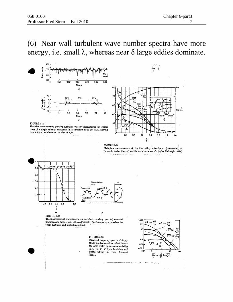
Fig. below shows measurements of turbulence for

Rex=107.

Note the following mean-flow features:

(1) Fluctuations are large ~ 11% U∞

(2) Presence of wall causes anisotropy, i.e., the

fluctuations differ in magnitude due to geometric and

physical reasons. 2'u is largest, 2'v is smallest and reaches

its maximum much further out than 2'u or 2'w . 2'w is

intermediate in value.

(3) 0'' vu and, as will be discussed, plays a very

important role in the analysis of turbulent shear flows.

(4) Although 0ji

uu at the wall, it maintains large values

right up to the wall

(5) Turbulence extends to y > δ due to intermittency.

The interface at the edge of the boundary layer is called

the superlayer. This interface undulates randomly

between fully turbulent and non-turbulent flow regions.

The mean position is at y ~ 0.78 δ.



(6) Near wall turbulent wave number spectra have more

energy, i.e. small λ, whereas near δ large eddies dominate.



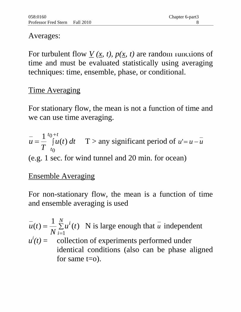
Averages:

For turbulent flow V (x, t), p(x, t) are random functions of

time and must be evaluated statistically using averaging

techniques: time, ensemble, phase, or conditional.

Time Averaging

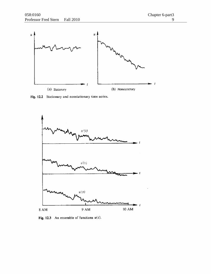
For stationary flow, the mean is not a function of time and

we can use time averaging.

tt

t

dttuT

u0

0

)(1

T > any significant period of uuu '

(e.g. 1 sec. for wind tunnel and 20 min. for ocean)

Ensemble Averaging

For non-stationary flow, the mean is a function of time

and ensemble averaging is used

N

i

i tuN

tu1

)(1

)( N is large enough that u independent

ui(t) = collection of experiments performed under

identical conditions (also can be phase aligned

for same t=o).



Phase and Conditional Averaging

Similar to ensemble averaging, but for flows with

dominant frequency content or other condition, which is

used to align time series for some phase/condition. In this

case triple velocity decomposition is used: ''' uuuu

where u΄΄ is called organized oscillation.

Phase/conditional averaging extracts all three

components.

Averaging Rules:

'fff 'ggg s = x or t

0'f ff gfgf 0' gf

gfgf f f

s s

''gfgffg

dsfdsf



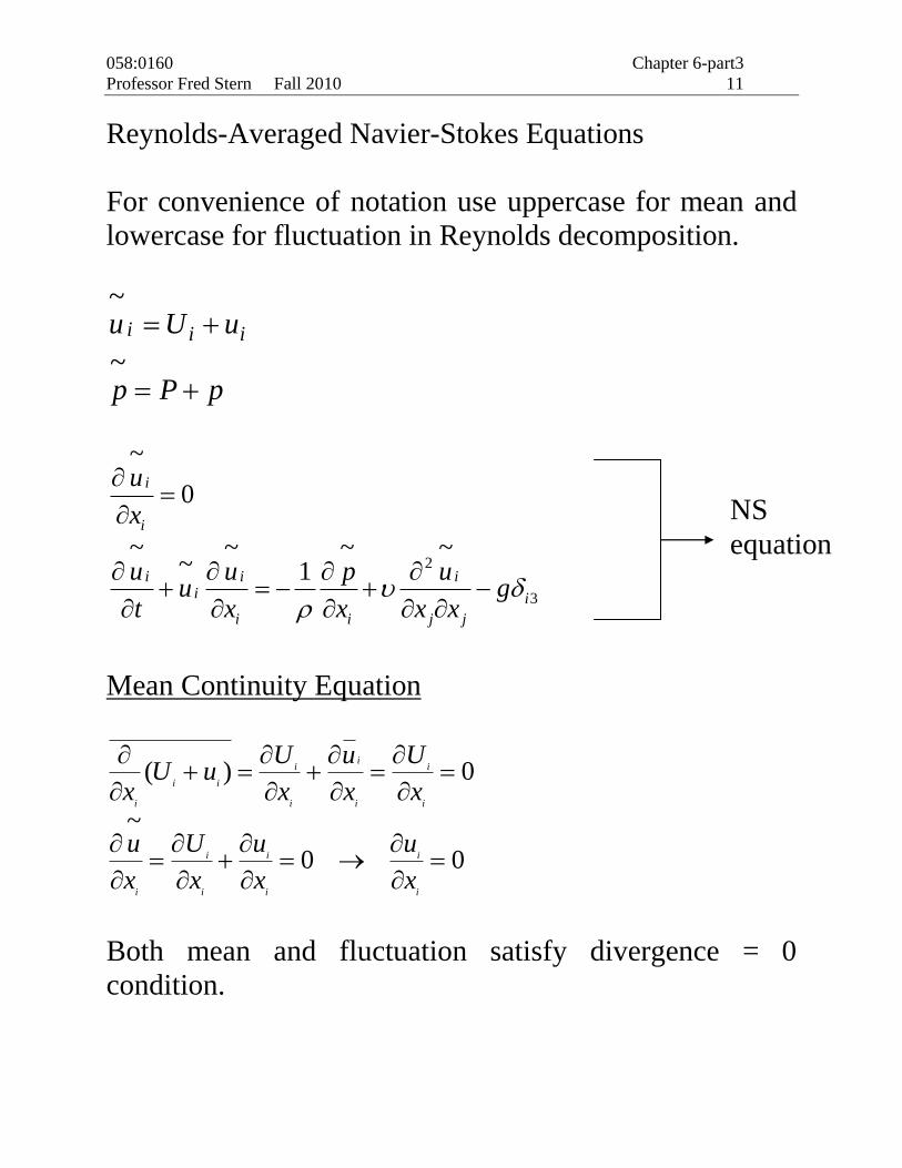
Reynolds-Averaged Navier-Stokes Equations

For convenience of notation use uppercase for mean and

lowercase for fluctuation in Reynolds decomposition.

pPp

uUu iii

~

~

2

3

~

0

~ ~ ~ ~~ 1

i

i

i i ii i

i i j j

u

x

u u p uu g

t x x x x

Mean Continuity Equation

00

~

0)(

i

i

i

i

i

i

i

i

i

i

i

i

i

ii

i

x

u

x

u

x

U

x

u

x

U

x

u

x

UuU

x

Both mean and fluctuation satisfy divergence = 0

condition.

NS

equation



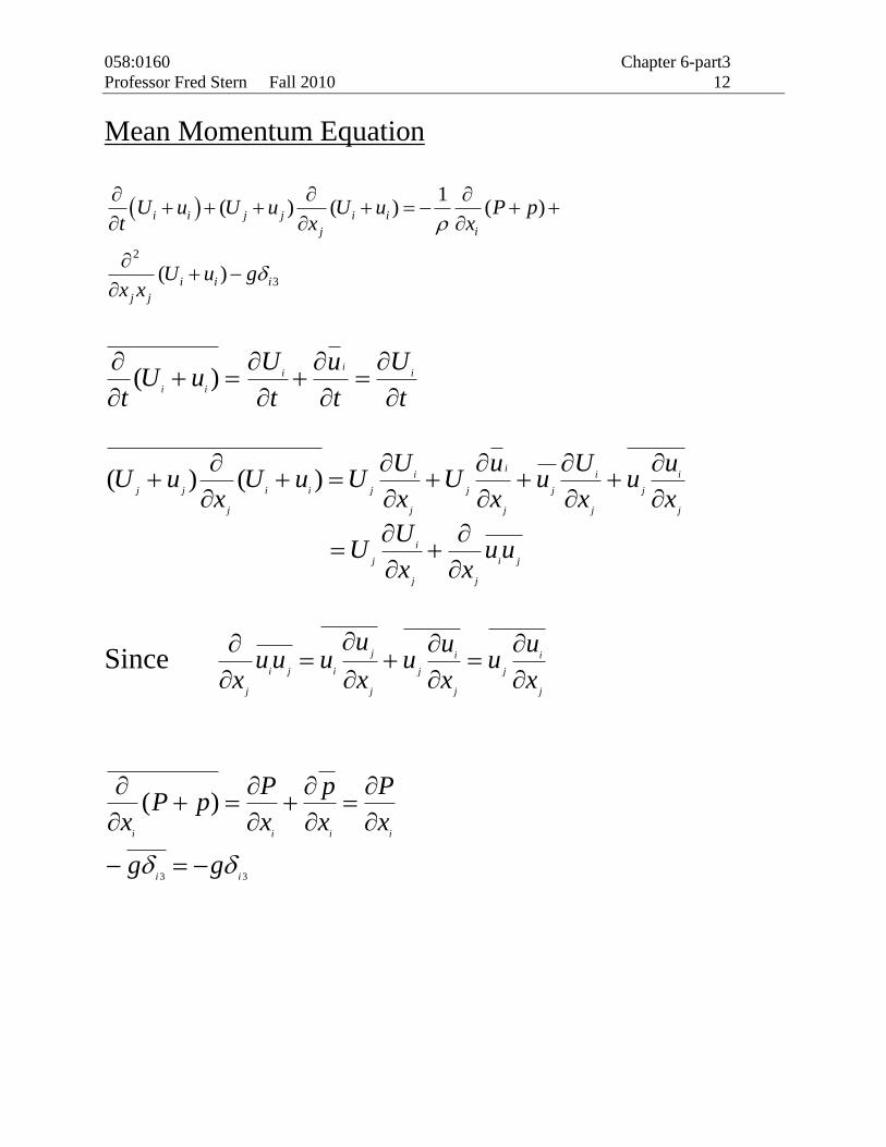
Mean Momentum Equation

2

3

1( ) ( ) ( )

( )

i i j j i i

j i

i i i

j j

U u U u U u P pt x x

U u gx x

t

U

t

u

t

UuU

t

ii

i

ii

)(

j

i

j

j

i

j

j

i

j

j

i

jii

j

jj

x

uu

x

Uu

x

uU

x

UUuU

xuU

)()(

ji

jj

i

juu

xx

UU

Since j

i

j

j

i

j

j

j

iji

jx

uu

x

uu

x

uuuu

x

33

)(

ii

iiii

gg

x

P

x

p

x

PpP

x



2

2

2

2

2

2

2

2

)(j

i

j

i

j

iii

j x

U

x

u

x

UuU

x

32

21)(ii

jij

ji

j

ij

i gUxx

P

x

uu

x

UU

t

U

Or

ji

j

i

ji

i

i uux

U

xg

x

P

Dt

DU

3

1

Or iji

ii

xg

Dt

DU

13

ji

i

j

j

i

ijuu

x

U

x

UP

with 0

i

i

x

U

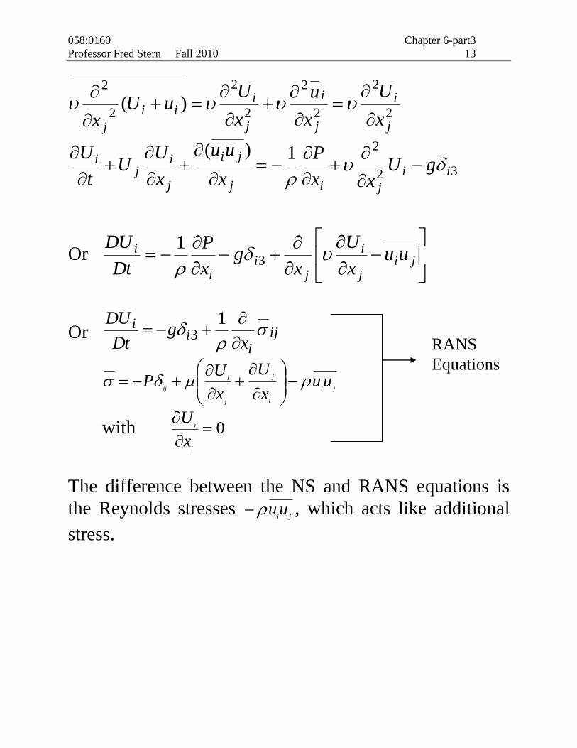
The difference between the NS and RANS equations is

the Reynolds stresses ji

uu , which acts like additional

stress.

RANS

Equations



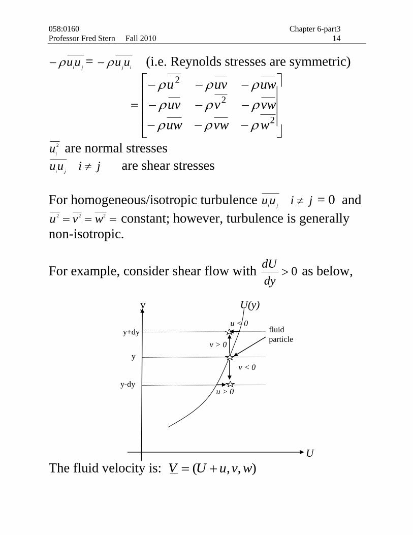
jiuu =

ijuu (i.e. Reynolds stresses are symmetric)

2

2

2

wvwuw

vwvuv

uwuvu

2

iu are normal stresses

jiuuji

are shear stresses

For homogeneous/isotropic turbulence jiuuji

= 0 and

222 wvu constant; however, turbulence is generally

non-isotropic.

For example, consider shear flow with 0dy

dU as below,

The fluid velocity is: ),,( wvuUV

y-dy

y

y+dy

y

U

U(y)

v > 0

v < 0

u > 0

u < 0 fluid

particle



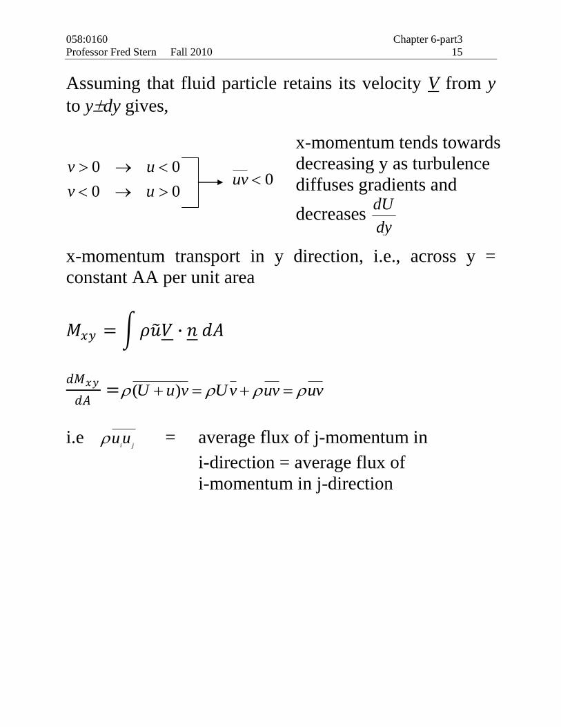
Assuming that fluid particle retains its velocity V from y

to ydy gives,

00

00

uv

uv 0uv

x-momentum transport in y direction, i.e., across y =

constant AA per unit area

𝑀𝑥𝑦 = 𝜌𝑢 𝑉 ∙ 𝑛 𝑑𝐴

𝑑𝑀𝑥𝑦

𝑑𝐴= uvuvvUvuU )(

i.e ji

uu = average flux of j-momentum in

i-direction = average flux of

i-momentum in j-direction

x-momentum tends towards

decreasing y as turbulence

diffuses gradients and

decreases dy

dU



Closure Problem:

1. RANS equations differ from the NS equations due to

the Reynolds stress terms

2. RANS equations are for the mean flow ( , )iU P ; thus,

represent 4 equations with 10 ten unknowns due to

the additional 6 unknown Reynolds stresses i ju u

3. Equations can be derived for i ju u by summing

products of velocity and momentum components

and time averaging, but these include additionally 10

triple product i j lu u u unknowns. Triple products

represent Reynolds stress transport.

4. Again equations for triple products can be derived

that involve higher order correlations leading to fact

that RANS equations are inherently non-

deterministic, which requires turbulence modeling.

5. Turbulence closure models render deterministic

RANS solutions.

6. The NS and RANS equations have paradox that NS

equations are deterministic but have

nondeterministic solutions for turbulent flow due to

inherent stochastic nature of turbulence, whereas the

RANS equations are nondeterministic, but have

deterministic solutions due to turbulence closure

models.



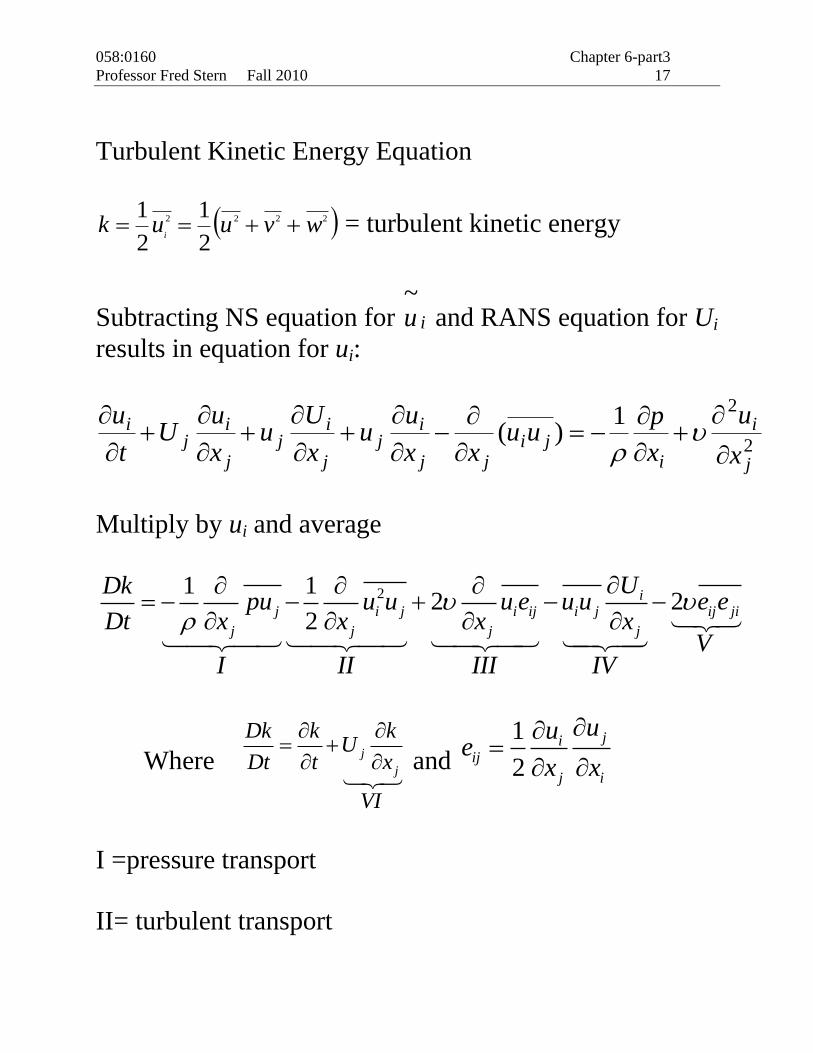
Turbulent Kinetic Energy Equation

2222

2

1

2

1wvuuk

i = turbulent kinetic energy

Subtracting NS equation for iu~

and RANS equation for Ui

results in equation for ui:

2

21

)(j

i

iji

jj

ij

j

ij

j

ij

i

x

u

x

puu

xx

uu

x

Uu

x

uU

t

u

Multiply by ui and average

21 12 2

2

ij i j i ij i j ij ji

j j j j

UDkpu u u u e u u e e

Dt x x x xV

I II III IV

Where j

j

Dk k kU

Dt t x

VI

and

1

2

jiij

j i

uue

x x

I =pressure transport

II= turbulent transport



III=viscous diffusion

IV = shear production (usually > 0) represents loss of

mean kinetic energy and gain of turbulent kinetic energy

due to interactions of ji

uu and j

i

x

U

.

V = viscous dissipation = ε

VI= turbulent convection

Recall previous discussions of energy cascade and

dissipation:

Energy fed from mean flow to largest eddies and cascades

to smallest eddies where dissipation takes place

Kinetic energy = k = uo2

0

3

0

0

2

0

l

uu

l0 = Lδ = width of flow (i.e. size of

largest eddy)

Kolmogorov Hypothesis:

(1) local isotropy: for large Re, micro-scale ℓ << ℓ0

turbulence structures are isotropic.



(2) first similarity: for large Re, micro-scale has

universal form uniquely determined by υ and ε.

4/13 / length 4/30 Re/ l

4/1 u velocity

4/10 Re/ uu

2/1/ time

2/1

0 Re/

Also shows that as Re increases, the range of scales

increase.

(3) second similarity: for large Re, intermediate scale

has a universal form uniquely determined by ε and

independent of υ.

(2) and (3) are called universal equilibrium range in

distinction from non-isotropic energy-containing range.

(2) is the dissipation range and (3) is the inertial subrange.

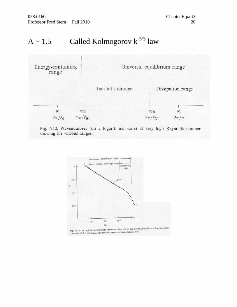
Spectrum of turbulence in the inertial subrange

0

2 )( dkkSu k = wave number in inertial subrange.

3/53/2 kAS For 1 1

0l k (based on dimensional analysis)

Micro-scale<<large scale



A ~ 1.5 Called Kolmogorov k-5/3 law



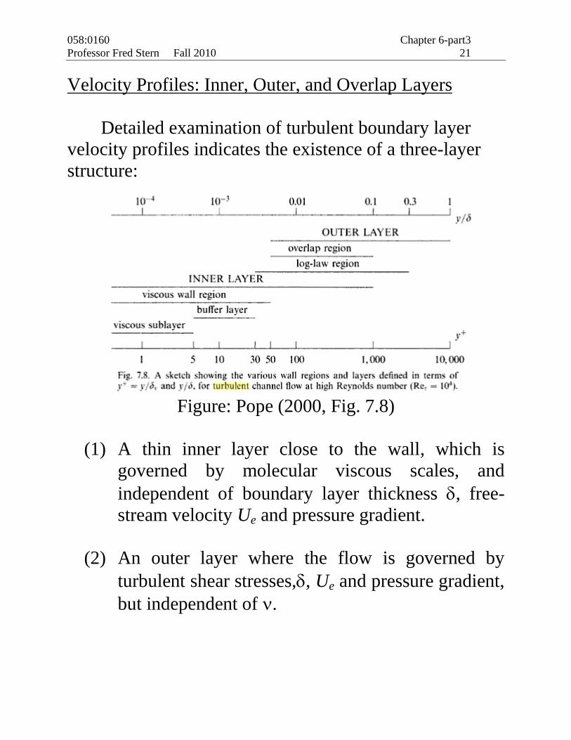
Velocity Profiles: Inner, Outer, and Overlap Layers

Detailed examination of turbulent boundary layer

velocity profiles indicates the existence of a three-layer

structure:

Figure: Pope (2000, Fig. 7.8)

(1) A thin inner layer close to the wall, which is

governed by molecular viscous scales, and

independent of boundary layer thickness , free-

stream velocity Ue and pressure gradient.

(2) An outer layer where the flow is governed by

turbulent shear stresses,, Ue and pressure gradient,

but independent of .



(3) An overlap layer which smoothly connects inner

and outer regions. In this region both molecular

and turbulent stresses and pressure gradient are

important.

Considerable more information is obtained from the

dimensional analysis and confirmed by experiment.

Inner layer: 𝑈 = 𝑓(𝜏𝑤 ,𝜌, 𝜇,𝑦)

𝑈+ =𝑈

𝑢∗ = 𝑓(𝑦𝑢∗

𝜈) /*

wu

)( yf

U+, y+ are called inner-wall variables

Note that the inner layer is independent of δ or r0, for

boundary layer and pipe flow, respectively.

Outer Layer: 𝑈𝑒 − 𝑈 𝑣𝑒𝑙𝑜𝑐𝑖𝑡𝑦 𝑑𝑒𝑓𝑒𝑐𝑡

= 𝑔(𝜏𝑤 ,𝜌,𝑦, 𝛿) for px = 0

𝑈𝑒−𝑈

𝑢∗ = 𝑔(𝜂) where /y

Note that the outer wall is independent of μ.

Wall shear

velocity



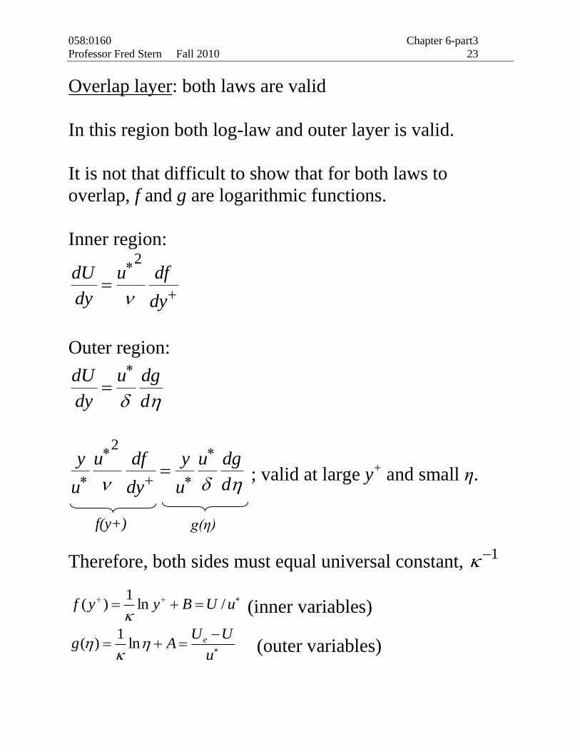
Overlap layer: both laws are valid

In this region both log-law and outer layer is valid.

It is not that difficult to show that for both laws to

overlap, f and g are logarithmic functions.

Inner region:

dy

dfu

dy

dU

2

Outer region:

d

dgu

dy

dU

d

dgu

u

y

dy

dfu

u

y

2

; valid at large y+ and small η.

Therefore, both sides must equal universal constant, 1

uUByyf /ln1

)(

(inner variables)

u

UUAg e

ln

1)( (outer variables)

f(y+) g(η)



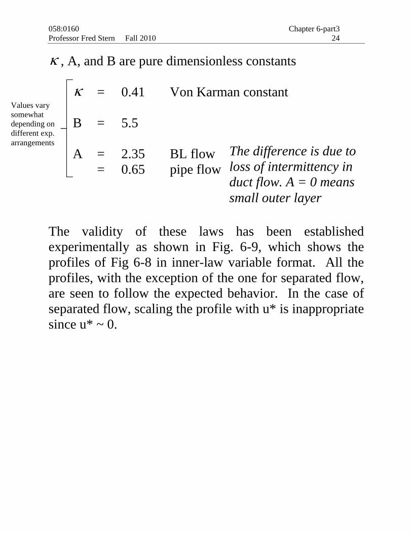
, A, and B are pure dimensionless constants

= 0.41 Von Karman constant

B = 5.5

A = 2.35 BL flow

= 0.65 pipe flow

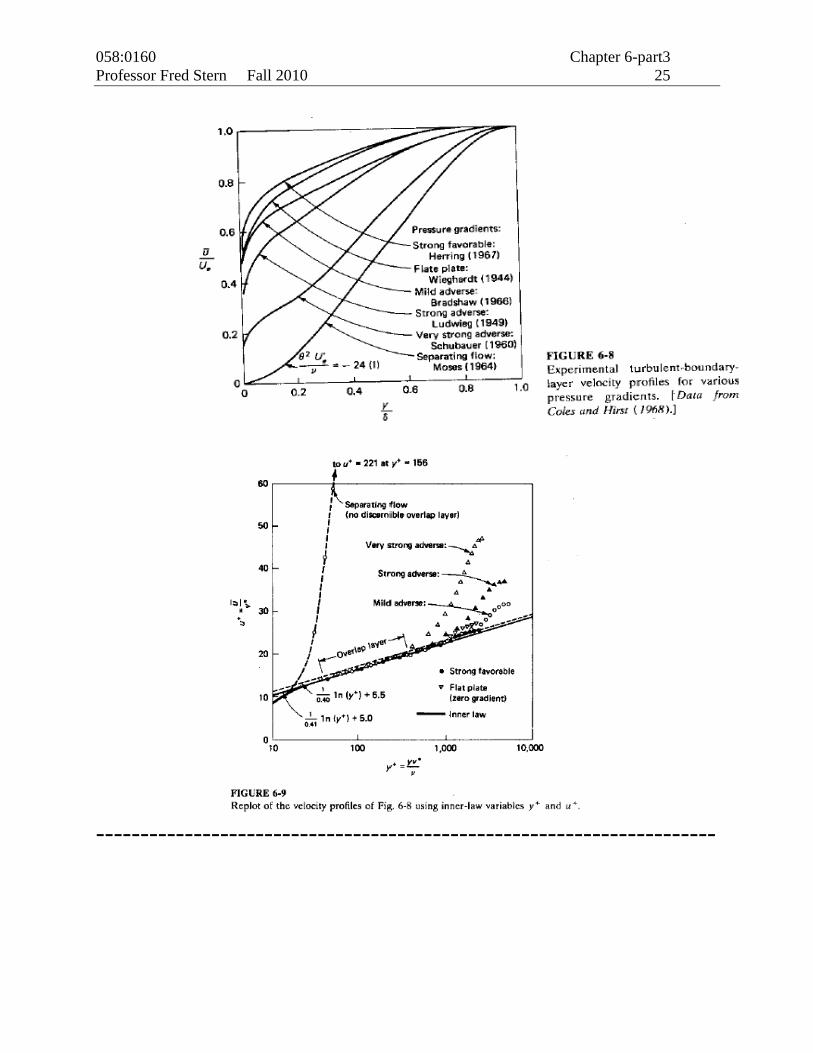
The validity of these laws has been established

experimentally as shown in Fig. 6-9, which shows the

profiles of Fig 6-8 in inner-law variable format. All the

profiles, with the exception of the one for separated flow,

are seen to follow the expected behavior. In the case of

separated flow, scaling the profile with u* is inappropriate

since u* ~ 0.

Values vary

somewhat

depending on

different exp.

arrangements

The difference is due to

loss of intermittency in

duct flow. A = 0 means

small outer layer



----------------------------------------------------------------------



Details of Inner Layer

Neglecting inertia and pressure forces in the 2D turbulent

boundary layer equation we get:

𝑑

𝑑𝑦(𝜇

𝑑𝑈

𝑑𝑦 − 𝜌𝑢𝑣 ) = 0

𝜇 𝑑𝑈

𝑑𝑦 − 𝜌𝑢𝑣 = 𝜏𝑡

The total shear stress is the sum of viscous and turbulent

stresses. Very near the wall y0, the turbulent stress

vanishes

lim𝑦→0

𝜇 𝑑𝑈

𝑑𝑦 − 𝜌𝑢𝑣 = 𝜇

𝑑𝑈

𝑑𝑦 𝑦=0

= 𝜏𝑤 = 𝜏𝑡

𝜇 𝑑𝑈

𝑑𝑦 − 𝜌𝑢𝑣 = 𝜏𝑤 (1)

Sublayer region: Very near the wall y0,

𝜏𝑤 = 𝜇 𝑑𝑈

𝑑𝑦 𝑦=0

(2)

From the inner layer velocity profile:



𝑑𝑈

𝑑𝑦 𝑦=0

= 𝑢∗2

𝜈

𝑑𝑓 (𝑦+)

𝑑𝑦+ (3)

Comparing equations (2) and (3) we get,

𝑑𝑓 (𝑦+)

𝑑𝑦+ = 1 𝑓 𝑦+ = 𝑦+ + 𝐶 (4)

No slip condition at y = 0 requires 𝐶 = 0.

Log-layer region: The molecular stresses are negligible

compared to turbulent stresses, thus

𝜏𝑤 = −𝜌𝑢𝑣 = 𝜇𝑡𝑑𝑈

𝑑𝑦 (6)

𝜇𝑡 is modeled using velocity gradient for time scale and

distance from wall as length scale (𝜅𝑦),

𝜇𝑡 = 𝜅𝑦 2 𝑑𝑈

𝑑𝑦 (7)

which gives:

Sublayer: U+ = y+ valid for y+ ≤ 5 (5)



−𝑢𝑣 = 𝜅𝑦 2 𝑑𝑈

𝑑𝑦

2 (8)

From inner layer velocity profile and equations (6) and

(8) we get,

𝑑𝑓 (𝑦+)

𝑑𝑦+ =𝜈

𝜅𝑦𝑢∗ = 1

𝜅𝑦+ (9)

𝑓 𝑦+ =1

𝜅ln 𝑦+ + 𝐶 (10)

Buffer layer: Merges smoothly the viscosity-dominated

subb-layer and turbulence-dominated log-layer in the

region 5< y+ ≤ 30.

Unified Inner layer: There are several ways to obtain

composite of sub-/buffer and log-layers.

Evaluating the RANS equation near the wall using μt

turbulence model shows that:

μt ~ y3 y 0

Several expressions which satisfy this requirement have

been derived and are commonly used in turbulent-flow

analysis. That is:

Log-law: U+ = 1

𝜅ln 𝑦+ + 𝐵 valid for y+ > 30 (11)



21

2U

Uee UB

t

(12)

Assuming the total shear is constant very near to the wall

as shown in equation (1), equation (12) can be integrated

to obtain a composite formula which is valid in the sub-

layer, blending layer, and logarithmic-overlap regions.

621

32UU

UeeyU uB

(13)

Fig. 6-11 shows a comparison of equation (13) with

experimental data obtained very close to the wall. The

agreement is excellent. It should be recognized that

obtaining data this close to the wall is very difficult.

----------------------------------------------------------------------



Alternative derivation of Overlap layer:

From the log law: 𝑑𝑈

𝑑𝑦=

𝑢∗

𝜅𝑦

From the outer layer:

d

dgu

dy

dU

Comparing the log-law and outer layer, we get

𝑑g

𝑑𝜂=

1

𝜅𝜂

u

UUAg e

ln

1)( (outer variables)

----------------------------------------------------------------------

Details of the Outer Law

At the end of the overlap region the velocity defect is

given approximately by:

𝑈𝑒−𝑈

𝑢∗ = 9.6(1 − 𝜂)2 (14)



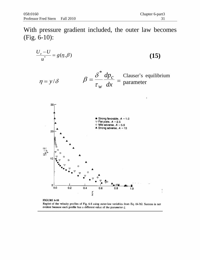
With pressure gradient included, the outer law becomes

(Fig. 6-10):

),(*

gu

UUe

(15)

/y dx

dpc

w

*

=

Clauser’s equilibrium

parameter



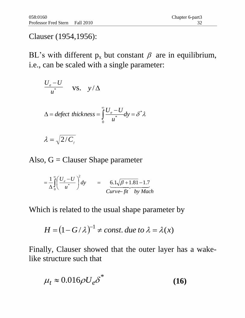
Clauser (1954,1956):

BL’s with different px but constant are in equilibrium,

i.e., can be scaled with a single parameter:

*u

UUe vs. /y

*

0

*

dyu

UUthicknessdefect e

f

C/2

Also, G = Clauser Shape parameter

MachbyfitCurve

dyu

UU e

7.181.11.61

0

2

*

Which is related to the usual shape parameter by

)(./11

xtodueconstGH

Finally, Clauser showed that the outer layer has a wake-

like structure such that

*016.0 et U (16)



Mellor and Gibson (1966) combined (15) and (16) into a

theory for equilibrium outer law profiles with excellent

agreement with experimental data: Fig. 6-12

Coles (1956):

A weakness of the Clauser approach is that the

equilibrium profiles do not have any recognizable shape.

This was resolved by Coles who showed that:

)/(2

1

5.5ln5.2

5.5ln5.2

yW

U

yU

e

(17)

Max deviation at δ Single wake-like function of y/δ

Deviations above log-overlap layer



fitcurve

yfunctionwakeW

2sin2 2 32 23 , /y

Thus, from (17), it is possible to derive a composite which

covers both the overlap and outer layers, as shown in Fig.

6-13.

)/(ln1

yWByU

parameterwake = π(β)

75.0)5.0(8.0 (curve fit for data)

Note the agreement of Coles’ wake law even for β

constant. Bl’s is quite good.



We see that the behavior in the outer layer is more

complex than that of the inner layer due to pressure

gradient effects. In general, the above velocity profile

correlations are extremely valuable both in providing

physical insight and in providing approximate solutions

for simple wall bounded geometries: pipe, channel flow

and flat plate boundary layer. Furthermore, such

correlations have been extended through the use of

additional parameters to provide velocity formulas for use

with integral methods for solving the BL equations for

arbitrary px.

Summary of Inner, Outer, and Overlap Layers

Mean velocity correlations

Inner layer:

)( yfU */ uUU

uyy / /*wu

Sub-layer: U+ = y+ for 50 y

Buffer layer: where sub-layer merges smoothly with

log-law region for 305 y



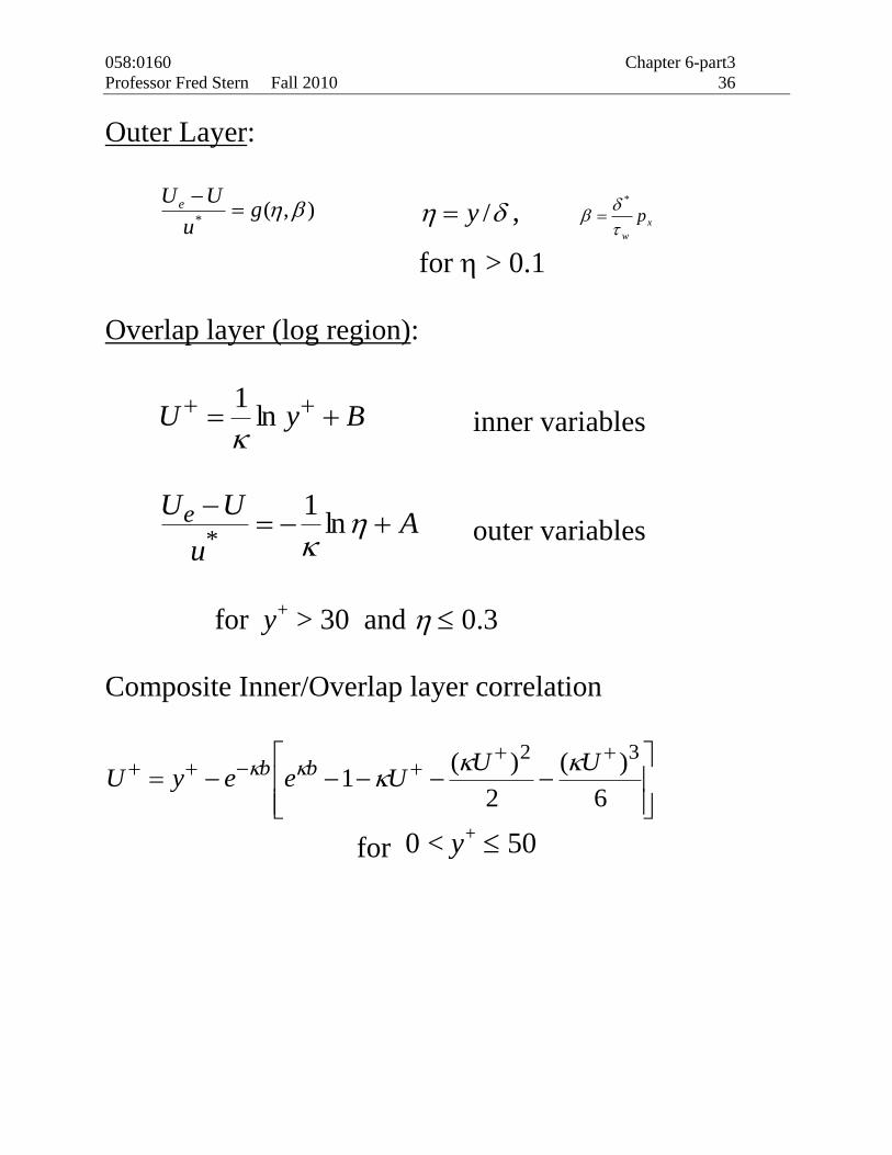
Outer Layer:

),(*

gu

UUe

/y , x

w

p

*

for > 0.1

Overlap layer (log region):

ByU ln1

inner variables

Au

UUe

ln1

* outer variables

for y+ > 30 and 0.3

Composite Inner/Overlap layer correlation

6

)(

2

)(1

32 UUUeeyU bb

for 0 < y+ 50



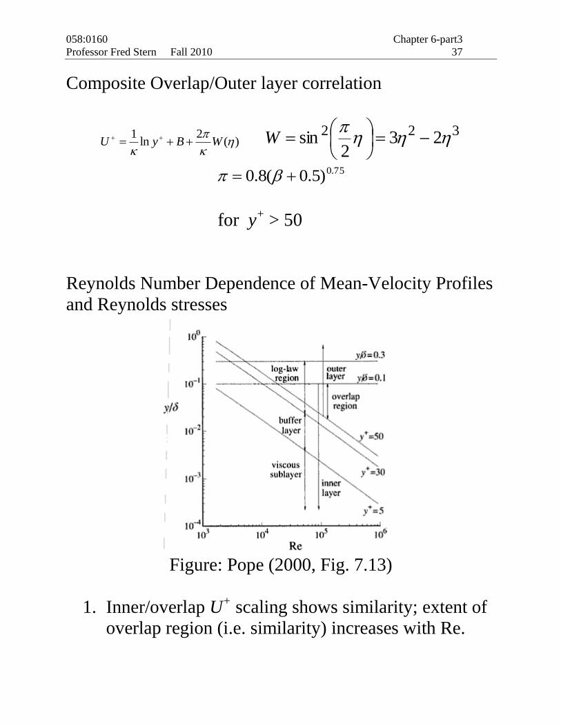
Composite Overlap/Outer layer correlation

)(2

ln1

WByU

322 232

sin

W

75.0)5.0(8.0

for y+ > 50

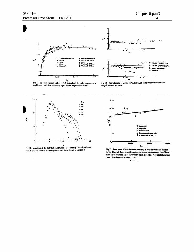
Reynolds Number Dependence of Mean-Velocity Profiles

and Reynolds stresses

Figure: Pope (2000, Fig. 7.13)

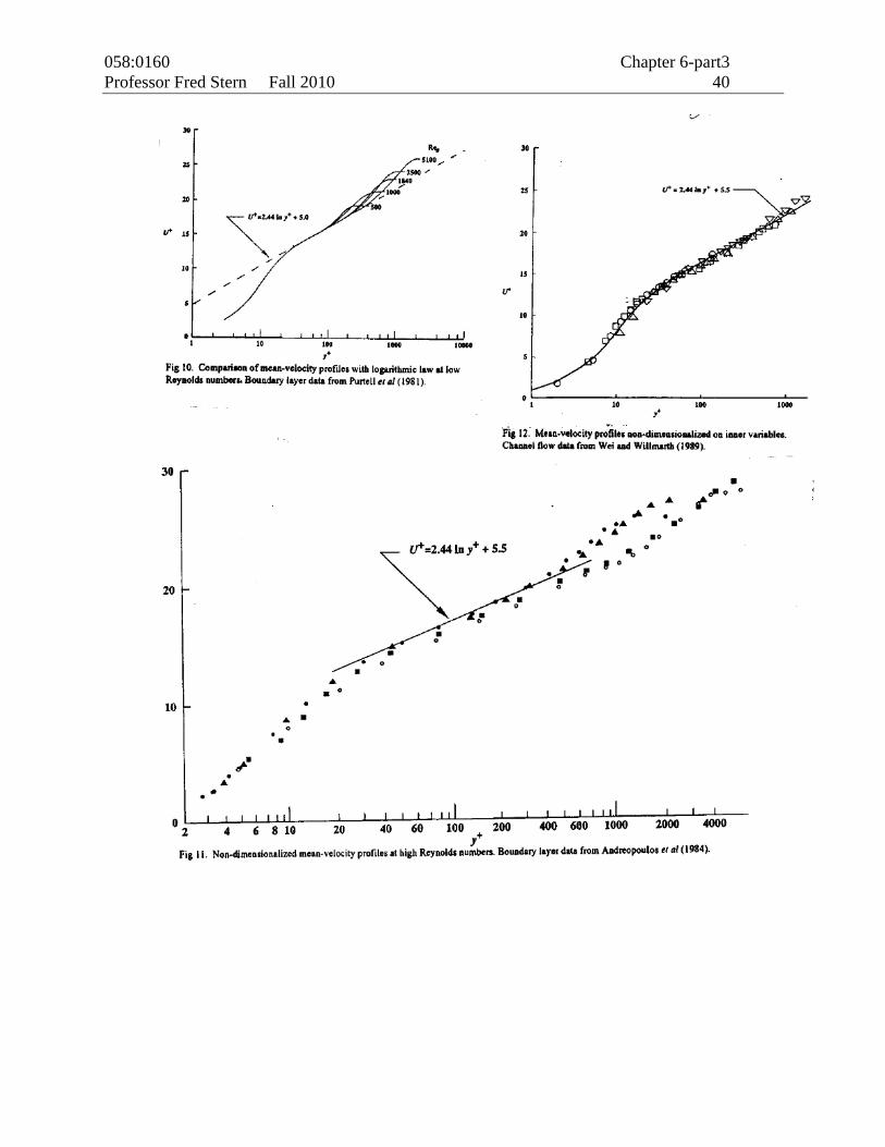
1. Inner/overlap U+ scaling shows similarity; extent of

overlap region (i.e. similarity) increases with Re.



2. Outer layer for px = 0 may asymptotically approach

similarity for large Re as shown by )/2( kU vs.

Reθ, but controversial due to lack of data for Reθ 5 x

104.

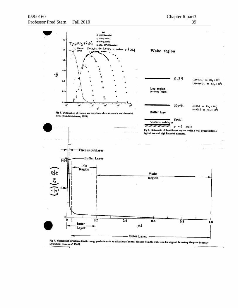
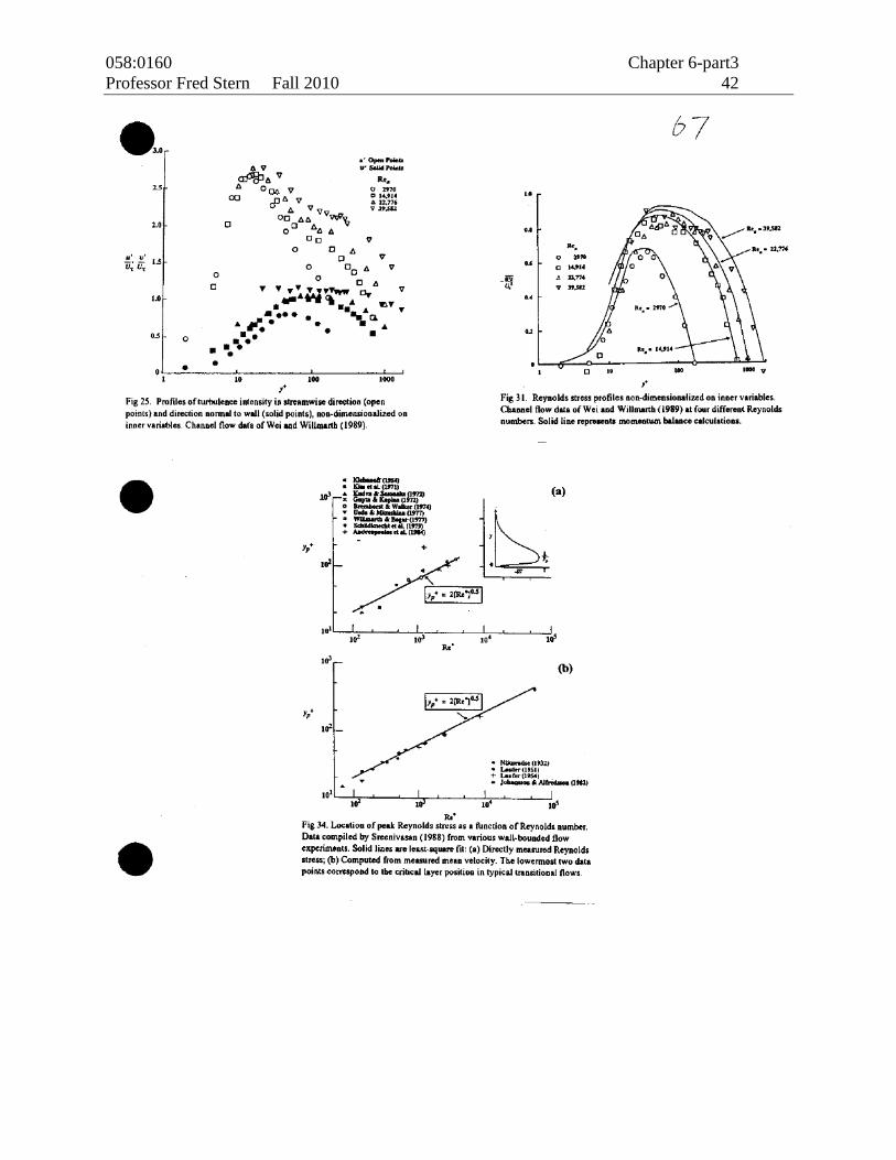
3. The normalized Reynolds stresses 𝑢𝑖𝑢𝑗 /𝑘,

production-dissipation ratio and the normalized

mean shear stress are somewhat uniform in the log-

law region. Experiments in flat plate boundary layer,

pipe and channel flow shows k = 3.34 - 3.43 u*2 in

lower part of log-law region.

4. Decay of k ~ y2 near the wall.

5. Streamwise turbulence intensity *

2

uuu vs. y+

shows similarity for 150 y (i.e., just beyond the

point of kmax, y+ = 12), but u+ increases with Reθ.

Chapter 6: Viscous Flow in Ducts

Documents

Transcript of Chapter 6: Viscous Flow in Ducts