CHAPTER 6 Thermogravimetric (TG/ DTA) Analysis of SnSeFe...
33
232 CHAPTER – 6 Thermogravimetric (TG/ DTA) Analysis of SnSeFe X (X = 0, 0.5, 1.0, 1.5, 2.0 & 2.5) Nanoparticles
Transcript of CHAPTER 6 Thermogravimetric (TG/ DTA) Analysis of SnSeFe...
232
CHAPTER – 6
Thermogravimetric (TG/ DTA)
Analysis of SnSeFeX
(X = 0, 0.5, 1.0, 1.5, 2.0 & 2.5)
Nanoparticles

233
6.1 Introduction
Materials sometimes lose its performance due to thermal,
chemical, or mechanical degradation. It has become necessary to
understand the environmental impact of its degradation and also its
effect on material properties. If the rate of degradation can be accurately
measured, then it becomes possible to predict the material properties. In
general, thermal analysis can provide important information on the
temperature dependent properties of materials and on thermally induced
processes (phase transition, decomposition, etc.). Thermal analysis is
advantageous it gives a general view of the thermal behaviour of a
material under various conditions and requires a small amount of
sample. The term thermal analysis can be applied to any technique
which involves the measurement of a physical quantity while the
temperature is changed or maintained in a controlled and measured
fashion. Usually the temperature is, for simplicity, kept constant or
increased linearly with time [1]. The International Confederation for
Thermal Analysis and Calorimetry (ICTAC) defines Thermal Analysis (TA)
as a group of techniques in which a property of the sample is monitored
against time or temperature while the temperature of the sample, in a
specified atmosphere, is programmed. The program may involve heating
or cooling at a fixed (or variable) rate of temperature change, or holding
the temperature constant, or any sequence of these. Since hardly any
measurement worth doing if the temperature is not controlled, almost all
measurements are some type of thermal analysis [1].
6.1.1 Classification of Individual Thermoanalytical Techniques
Thermometry, is the simplest technique of thermal analysis. It
becomes even more useful when time is recorded simultaneously. Such
thermal analyses are called heating or cooling curves. Time is measured
with a clock, temperature with a thermometer.

234
The most basic thermal analysis technique is naturally
calorimetry, the measurement of heat. The needed thermal analysis
instrument is the calorimeter. Intermediate between thermometry and
calorimetry is Differential Thermal Analysis (DTA). In this technique
transition temperature information is derived by the qualitative changes
in heats of transition or heat capacity. As the instrumentation of DTA
advanced, quantitative heat information could be derived from
temperature and time measurements. The DTA has in the last 50 years
increased so much in precision that its applications overlap with
calorimetry.
The basic measurement of length or volume is called dilatometry if
it is carried out at constant pressure or stress. When measuring stress
as well as strain, the technique is called Thermo Mechanical Analysis,
(TMA). Measurements can be made at constant or variable stress or
strain, including periodic changes as in dynamic mechanical analysis.
Finally, Thermogravimetric Analysis or Thermal Gravimetric Analysis
(TGA) is a method of thermal analysis in which changes in physical and
chemical properties of materials are measured as a function of increasing
temperature (with constant heating rate), or as a function of time (with
constant temperature and/or constant mass loss) [2]. TGA can be used
to evaluate the thermal stability of a material. In a desired temperature
range, if a species is thermally stable, there will be no observed mass
change. Negligible mass loss corresponds to little or no slope in the TGA
trace. TGA also gives the upper use temperature of a material. Beyond
this temperature the material will begin to degrade.
Several more complicated thermal analysis techniques are
mentioned from time to time, described in Table 6.1 which involve
additional specialization, also mentioned in addition of time and
temperature. These various techniques can define for future development
in device fabrication by studying stability and to find out thermal

235
parameters by thermal characterization. The arrangement finally adopted
for the defined techniques (Table 6.1) incorporate additional physical
properties and/or techniques as necessary: various modes of certain
techniques can also be distinguished.
The confusion that has arisen about this term is resolved by
separating two modes (Power compensation DSC and Heat-flux DSC) as
described in the definition given in the text.
Table 6.1: Classification of Thermoanalytical Techniques.
Physical Property Derived Technique
Mass
Thermogravimetry (TG)
Isobaric mass change determination
Evolved Gas Detection (EGD)
Evolved Gas Analysis (EGA)
Emanation Thermal Analysis (ETA)
Temperature Heating or cooling curve determination
Differential Thermal Analysis (DTA)
Enthalpy Differential Scanning Calorimetry (DSC)
Dimensions Thermodiliatometry
Mechanical
characteristics
Thermochemical measurements
Dynamic Thermochemical measurements
Acoustic characteristic Thermosonimetry
Thermoacoustimetry
Optical characteristic Thermoptometry
Electrical characteristic Thermoelectrometry
Magnetic characteristic Thermomagnetometry

236
6.1.2 Thermogravimetry
Thermogravimetric analysis covers a wide spectrum of thermo
analytical techniques, which monitor one or more physical properties of a
substance that is undergoing a temperature programmed heating as a
function of time and temperature. It provides a quantative measurement
of any weight changes associated with thermally associated changes.
Thermogravimetric analysers can be called as a thermo balance which is
a combination of a suitable electronic microbalance with a furnace,
which is operated with a computer controlled heating programme. It
allows the sample to be weighed and heated or cooled in a temperature
controlled manner and the mass, time and temperature data to be
recorded under specific atmosphere. The thermogravimetry analyzer
(TGA) system, which combines thermogravimetry (TG) and differential
thermal analyzer (DTA), is widely used in the fields of gas– solid
interactions, fuels, catalysis, polymers and chemical synthesis.
Thermogravimetric analysis is used to determine the material‟s thermal
stability and its fraction of volatile components by monitoring the weight
change that occurs as a sample is heated. This is explained later in
detail. The measurement is normally carried out in an inert atmosphere,
such as Helium or Argon, and the weight is recorded as a function of
temperature. In addition to weight changes, some instruments also
record the temperature difference between the specimen and the
reference pan (differential thermal analysis, or DTA) or the heat flow into
the specimen crucible compared to that of the reference crucible
(differential scanning calorimetry, or DSC). The latter can be used to
monitor the energy released or absorbed via chemical reactions during
the heating process.
A DTA apparatus consists of a sample holder comprising
thermocouples, sample containers and a ceramic or metallic block; a
furnace; a temperature programmer; and a recording system. The key

237
feature is the existence of two thermocouples connected to a voltmeter.
One thermocouple measures the temperature of an inert material such
as Al2O3, while the other is used for measurement for the sample
temperature under study. As the temperature is increased, there will be
a deflection of the voltmeter if the sample is undergoing a phase
transition. This occurs because the input of heat will raise the
temperature of the inert substance, but be incorporated as latent heat in
the material changing phase. In DTA, the differential temperature is
plotted against the time, or against the temperature (DTA curve or
thermogram). Changes in the sample, either exothermic or endothermic,
can be detected relative to the inert reference. Thus, a DTA curve
provides data on the transformations that have occurred, such as glass
transitions, crystallization, melting and sublimation. The area under a
DTA peak is related to the enthalpy change of the sample. Generally a
sharp endothermic (negative peak) DTA peak at particular temperature
indicates the melting point of the sample as the temperature of the
sample at this particular temperature would lag behind the temperature
of reference substance where as an exothermic peak indicate the onset of
decomposition process.
6.1.3 Thermogravimetric Analysis (TGA)
The thermal properties like heat capacities, the glass transition
temperature, melting and degradation of macromolecules can be
analyzed using thermogravimetry and differential thermal analysis along
with differential scanning calorimetry (DSC).
Thermal measurements are based on the measurement of dynamic
relationship between temperature and some property of a system such as
mass, heat of reaction or volume when the material is subjected to a
controlled temperature programme. In thermogravimetric analysis, the
mass of the sample is recorded continuously as a function of
238
temperature as it is heated or cooled at a controlled rate. A plot of mass
as a function of temperature is known as thermogram. The apparatus
required for thermo-gravimetric analysis include a sensitive recording
analytical balance, a furnace, a temperature controller, and a
programmer that provides a plot of the mass as a function of
temperature. Often an auxiliary equipment to provide an inert
atmosphere for the sample is also needed. Changes in the mass of the
sample occurs as a result of rapture and/or formation of various
physical and chemical bonds at elevated temperature that led to the
evolution of volatile products or formation of reaction products. Thus
TGA curve provides information regarding the thermodynamics and
kinetics of various chemical reactions, reaction mechanisms, and
intermediate and final reaction products.
6.1.4 Differential Thermal Analysis (DTA)
A technique in which the temperature difference between a
substance and a reference material is measured as a function of
temperature whilst the substance and reference material are subjected to
the same controlled temperature programme. The record is the
differential thermal or DTA curve; the temperature difference (ΔT) should
be plotted on the ordinate with endothermic reactions downwards and
temperature or time on the abscissa increasing from left to right. The
term quantitative differential thermal analysis i.e. Quantitative DTA,
cover those uses of DTA where the equipment is designed to produce
quantitative results in terms of energy and / or any other physical
parameter.
6.1.5 Thermal Analysis for Physical Significance
Thermal analysis refers to a group of techniques in which the
properties of a substance under study is monitored with respect to time
and temperature in a specified atmosphere. This is often done by heating

239
the precursors (starting materials) in an evaporator isothermally.
Volatization of solid in a broad sense includes any process which result
in conversion of matter from the solid state to the vapor phase.
Volatization process can be accomplished by two ways.
1. Sublimation process in which the gaseous phase composed of the
same type of atoms or molecules supplied by the solid phase i.e.
the composition of the gaseous phase and the solid phase remain
the same - a true vaporization process.
2. A chemical reaction between the solid phase and another species
to form gaseous products. The additional species may be
environmental gases, adsorbed water, or some some solid like
container material. In both cases the composition of the gaseous
phase is always different from the solid phase. This is often termed
as decomposition or pyrolysis.
As solid is heated, the extent of lattice vibrations within the solid are
increased and a temperature would be reached during heating where
following changes can occur:
Melting: the forces of attraction between the constituents decrease
which maintain an orderly arrangement of the solid and comes
down to a more disordered system called liquid state.
Phase transition: a new arrangement of the lattice structure.
Sublimation: direct transformation from the solid state to the gas
phase occurs.
Decomposition: sometimes the molecular rearrangements of bonds
within the solid during heating also result in formation products
chemically different from the solid. These products can be a solid
or gasses. This occurs over a range of temperature.

240
Thus by obtaining gravimetric data of heating a solid sample with
time or temperature in a specified atmosphere, one would easily predict
about the volatility, thermal stability and physical state of the sample at
a particular temperature.
Precisely determined thermodynamic events, such as a change of
state, can indicate the identity and purity of drugs. Compendia
standards have long been established for the melting or boiling
temperatures of substances. These transitions occur at characteristic
temperatures and the compendia standards therefore contribute to the
identification of the substances. Because impurities affect these changes
in predictable ways, the same compendial standards contribute to the
control of the purity of the substances.
Thermal analysis in the broadest sense is the measurement of
physical-chemical properties of materials as a function of temperature.
Instrumental methods have largely supplanted older methods dependent
on visual inspection and on measurements under fixed or arbitrary
conditions, because they are objective, they provide more information,
they afford permanent records, and they are generally more sensitive,
more precise, and more accurate. Furthermore, they may provide
information on crystal perfection, polymorphism, melting temperature,
sublimation, glass transitions, dehydration, evaporation, pyrolysis, solid
solid interactions, and purity. Such data are useful in the
characterization of substances with respect to compatibility, stability,
packaging, and quality control. The measurements used most often in
thermal analysis, i.e., transition temperature, thermogravimetry, and
impurity analysis, are described here.
Transition Temperature - As a specimen is heated, its uptake (or
evolution) of heat can be measured [Differential Scanning Calorimetry
(DSC)] or the resulting difference in temperature from that of an inert

241
reference heated identically [Differential Thermal Analysis (DTA)] can be
measured. Either technique provides a record of the temperature at
which phase changes, glass transitions, or chemical reactions occur. In
the case of melting, both an “onset” and a “peak” temperature can be
determined objectively and reproducibly, often to within a few tenths of a
degree. While these temperatures are useful for characterizing
substances, and the difference between the two temperatures is
indicative of purity, the values cannot be correlated with subjective,
visual “melting range” values or with constants such as the triple point of
the pure material.
6.1.6 Applications
TG Analysis gives us information about the thermal events which
are accompanied by changes in mass. For desorption, decomposition and
oxidation processes, useful information can be collected from TG
analysis. It gives accurate information about drying and the
decomposition of metal hydroxides into oxides in ferrite processing. The
mass losses define the stages and the conditions of temperature and
atmosphere necessary for the preparation of the spinel phase and the
stability. TG curves for complex ternary metal hydroxides like the present
study, may not give the exact reaction occurring even then it can be used
for “finger print‟ purposes [3]. Further it can be utilized for engine oil
volatility measurements, filler content, flammability studies, heat of
transition, oxidative stabilities, thermal stabilities, transition
temperatures and catalyst and coking studies.
6.2 Experimental
Simultaneous Thermogravimetric (TG) and Differential Thermal
(DT) analyses were carried out on a Rigaku thermobalance using about
10 mg of sample. Alumina was used as reference. Generally, these
experiments can be done either under Ar, He or N2 gas atmosphere or

242
without using gas (i.e. in air). Here author has performed TG/ DTA
experiment under air. A vacuum purge of atmospheric air was done
before starting the experiments. This operation induces a systematic
mass loss because, under vacuum, the samples start to lose water from
room temperature. A complete description of the conditions employed
should accompany each thermogram, including make and model of
instrument; record of last calibration; specimen size and identification
(including previous thermal history); container; identity, flow rate, and
pressure of gaseous atmosphere; direction and rate of temperature
change; and instrument and recorder sensitivity.
6.2.1 Construction and Working of Thermal Analyzer
A thermobalance is a combination of an electronic microbalance,
furnace and a temperature programmer. Figure 6.1(a) and Figure 6.1(b)
shows schematic thermobalance. The thermobalance is placed in an
enclosed system to control the atmosphere. The measurements of mass
changes with temperature are carried out with the help of such
thermobalance. The maximum load for thermobalance is 1g and a
sensitivity of 1μg.
The sample should be powdered where possible and should be
spread in a thin and uniform layer in the sample container.
Thermobalance is normally housed in a glass or metal systems to control
the pressure and the atmosphere inside it. A regular gaseous flow may be
maintained in order to remove the evolved gases from the thermobalance
with the care that these the flow gases don not disturb the balance [3].
Temperature sensors are either platinum resistance thermometers or
thermocouples. The temperature controller attached to the instrument
offer heating rates from a fraction of a degree per minute to nearly 100 °C
min-1 with additional characteristic of isothermal heating

243
(a) (b)
Figure 6.1 (a) & (b): A schematic thermobalance
The beam is displaced by change in weight loss with temperature
on sample side. This displacement is detected optically and the drive coil
current is changed to return the displacement to zero. The detected drive
coil current change is proportional to the amount of weight change in
sample and is output as the TG signal. The DTA detects the temperature
difference between the sample holder and the reference holder using
electromotive force of thermocouples, attached to the holders. The
differential is output as the DTA signal.
It is appropriate to make a preliminary examination over a wide
range of temperature (typically room temperature to decomposition
temperature or about 10°to 20 above the melting point) and over a wide
range of heating rates (2 to 20 per minute), which may reveal unexpected
effects; then a single examination or replicate examinations over a
narrow range, bracketing the transition of interest at one or more lower
heating rates, can be made. In examining pure crystalline materials,
rates as low as 1 per minute may be appropriate, whereas rates of up to
10 per minute are more appropriate for polymeric and other semi
crystalline materials. As the reliability of the measurements varies from

244
one substance to another, statements of the number of significant figures
to be used in the reporting of intralaboratory repeatability and of inter
laboratory reproducibility cannot be given here, but should be included
in the individual monograph.
Thermogravimetric analysis involves the determination of the mass
of a specimen as a function of temperature, or time of heating, or both,
and when properly applied, provides more useful information than does
loss on drying at fixed temperature, often for a fixed time and in what is
usually gas atmosphere. Usually, loss of surface absorbed solvent can be
distinguished from solvent in the sample and from degradation losses.
The measurements can be carried out in atmospheres having controlled
humidity and oxygen concentration to reveal interactions with the drug
substance, between drug substances, and between active substances
and excipients or packaging materials. While the details depend on the
manufacturer, the essential features of the equipment are a recording
balance and a programmable heat source. Equipment differs in the
ability to handle specimens of various sizes, the means of sensing
specimen temperature, and the range of atmosphere control. Calibration
is required with all systems, i.e., the mass scale is calibrated by the use
of standard weights; calibration of the temperature scale, which is more
difficult, involving either variations in positioning of thermocouples and
their calibration; or in other systems, calibration involves the use of
standard materials because it is assumed that the specimen temperature
is the furnace temperature.
Procedural details are specified in order to provide for valid
interlaboratory comparison of results. The specimen weight, source, and
thermal history are noted. The equipment description covers dimensions
and geometry, the materials of the test specimen holder, and the location
of the temperature transducer. Alternatively, the make and model
number of commercial equipment are specified. In all cases,
245
thecalibration record is specified. Data on the temperature environment
include the initial and final temperatures and the rate of change or other
details if nonlinear. The test atmosphere is critical; the volume, pressure,
composition, whether static or dynamic, and if the latter, the flow rate
and temperature are specified.
6.3 Results and Discussion
6.3.1 Broido and Coats Redfern (C – R) Method
Various researchers [4] put forward integral method, which can be
applied to thermogravimetric data assuming order of reaction and from
which the activation energy (Ea) can be estimated. In thermaogravimetric
measurement, the mass conversion is typically calculated as following
Equation 6.1.
0
0 f
m mY
m m
(6.1)
where y is fraction of initial molecules not yet decomposed and
equal to; m represents initial sample mass in an experiment, m denotes
current mass and mf represents final mass. Kinetic studies assume that
the isothermal rate of conversion, dy/dt, is a linear function of the
reactant concentration loss and of temperature independent function of
the conversion, y that is given by Equation 6.2.
( )dy
kf Ydt
(6.2)
where f = (Y) is the reaction model that depends on the mechanism
of degradation. The function ‘k’ is always described by Arrhenius
expression Equation 6.3 can be given by this way.
aE
RTk Ae
(6.3)

246
where A is pre exponential factor (also called as Arrhenius
constant), is assumed to be independent of temperature, E is activation
energy, T is absolute a temperature and R is universal gas constant. The
combination of equation 6.2 and 6.3 gives the following relationship i.e.
Equation 6.4.
( )aE
RTdy
Af Y edt
(6.4)
When temperature of sample is changed under controlled and
constant heating rate (dT/dt), the variation in degree of conversion of
mass can be analyzed as a function of temperature, which depends on
time of heating. Therefore, reaction rate may be written as follows
Equation 6.5.
dy dy dT dy
dt dT dt dt
(6.5)
Thus, change in mass vs temperature can be written as Equation 6.6.
( )aE
RTdy A
e f Ydt
(6.6)
Integral form of from Equation 6.6, initial temperature, to
corresponding to a degree of conversion m o to a peak temperature, Tp
can be written as Equation 6.7.
00 ( )
ap
EY T
RT
T
dY Ae dT
f Y
(6.7)
Using an approximation, Broido rearranged [5] the Equation 6.7
and obtained Equation 6.8 as followed.
2
max1ln ln a
a a
E RAT
Y RT E
(6.8)

247
In Broido’s approximation, the order of thermal degradation is
considered as first order and the calculations are done accordingly.
Assuming the order of equation, Coats and Redferd [6] developed an
integral method for analysis of thermogravimetric data as given below
Equation 6.9.
2
ln(1 ) 2ln ln 1 a
a a
EY RA RT
T E E RT
for n=1 (6.9)
The Horowitz and Metzger [7] modified the equation as below
Equation 6.10.
( )ln(1 )
( )
a p
p
E T TY
R T
for n=1 (6.10)
For both C- R and H- M methods, the correlation coefficient values
among the reaction of different orders are considered. The values of “y”
were determined at different temperature interval from TG curve of
instrument carried out. A plot of ln ln (1/y) in case of Broido’s method,
ln [-(1-y)/T2] in case of C- R method and (1- y) in case of H- M method;
versus 1000/ T for major degradation events yielded straight line and
slope. This slope is equal to – Ea/ 2.303 R [8]. Ea values of all the
samples are presented in Table 6.2 for pure and iron doped SnSe
nanoparticles.
After obtaining the energy of activation i.e. Ea value, from Broido
and Coats- Redfern method, the entropy of activation ΔS can be
calculated by following Equation 6.11.
lnB s
AhS R
k T
(6.11)
where kB is Boltzmann constant, h is Plank’s constant and Ts
peak temperature.

248
The enthalpy of activation (ΔH) and Gibbs free energy (ΔG) can be
calculated from following relationship i.e. Equation 6.12 and Equation
6.13.
H E RT (6.12)
G H T S (6.13)
In Results and discussion part, all these thermal parameters are
investigated by using two thermodynamical model and all the plots were
show good correlation coefficients.
Figure 6.2 (a):TG and DTA thermogram of SnSe nanoparticles.
Temp Cel10008006004002000
DT
A u
V
5.00
0.00
-5.00
-10.00
-15.00
-20.00
-25.00
-30.00
TG
%
100.0
90.0
80.0
70.0
60.0
50.0
40.0
DT
G u
g/m
in
70.00
60.00
50.00
40.00
30.00
20.00
10.00
0.00
43.6%
6.2%
5.7%
55.4%
35Cel
99.7%
247Cel
93.6%
559Cel
51.1%
940Cel
44.3%
85Cel
13.51ug/min
319Cel
24.43ug/min
450Cel
56.95ug/min
469Cel
61.05ug/min
581Cel
13.51ug/min
42Cel
0.00uV
841Cel
-31.63uV

249
Figure6.2 (b): TG and DTA thermogram of SnSeFe0.5 nanoparticles.
Figure 6.2 (c): TG and DTA thermogram of SnSeFe1.0 nanoparticles.
Temp Cel800.0600.0400.0200.00.0
DT
A u
V
20.00
10.00
0.00
-10.00
-20.00
-30.00
TG
%
100.0
90.0
80.0
70.0
60.0
50.0
40.0
30.0
DT
G u
g/m
in
200.0
150.0
100.0
50.0
0.0
-50.0
36.8%52.2%
76.9Cel
18.4ug/min
354.1Cel
43.0ug/min
373.7Cel
38.7ug/min
413.2Cel
65.4ug/min
447.8Cel
31.6ug/min
507.9Cel
47.1ug/min
657.8Cel
9.5ug/min
34.2Cel
99.4%
276.5Cel
91.1%
558.8Cel
54.9%936.8Cel
47.2%
41.3Cel
-0.33uV
866.9Cel
-28.45uV
940.3Cel
-27.87uV
Temp Cel800.0600.0400.0200.00.0
DT
A u
V
15.00
10.00
5.00
0.00
-5.00
-10.00
-15.00
TG
%
100.0
90.0
80.0
70.0
60.0
50.0
40.0
DT
G u
g/m
in
150.0
100.0
50.0
0.0
38.8% 53.3%
35.5Cel
99.0%
292.6Cel
91.0%
590.1Cel
53.2%
939.2Cel
45.8%
98.0Cel
16.3ug/min
350.9Cel
38.9ug/min
414.6Cel
58.2ug/min
499.3Cel
62.6ug/min
668.4Cel
13.9ug/min
48.9Cel
-0.09uV
595.5Cel
-12.29uV940.0Cel
-15.95uV

250
Figure 6.2 (d): TG and DTA thermogram of SnSeFe1.5 nanoparticles.
Figure 6.2 (e): TG and DTA thermogram of SnSeFe2.0 nanoparticles.
Temp Cel800.0700.0600.0500.0400.0300.0200.0100.00.0
DT
A u
V
10.00
5.00
0.00
-5.00
-10.00
-15.00
TG
%
100.0
95.0
90.0
85.0
80.0
75.0
70.0
65.0
60.0
55.0
50.0
45.0
DT
G u
g/m
in200.0
150.0
100.0
50.0
0.0
-50.0
-100.0
38.3%
9.5%
2.8%
29.8Cel
99.5%
278.0Cel
90.0%
592.2Cel
52.8%
749.5Cel
48.9%
50.6%
95.2Cel
35.2ug/min
323.2Cel
52.1ug/min
354.0Cel
80.4ug/min
367.8Cel
95.2ug/min
521.8Cel
90.5ug/min36.9Cel
0.33uV
602.3Cel
-14.30uV
Temp Cel600.0500.0400.0300.0200.0100.0
DT
A u
V
-2.00
-4.00
-6.00
-8.00
-10.00
-12.00
TG
mg
3.800
3.600
3.400
3.200
3.000
2.800
2.600
2.400
2.200
DT
G u
g/m
in
90.00
80.00
70.00
60.00
50.00
40.00
30.00
20.00
10.00

251
Figure 6.2 (f): TG and DTA thermogram of SnSeFe2.5 nanoparticles.
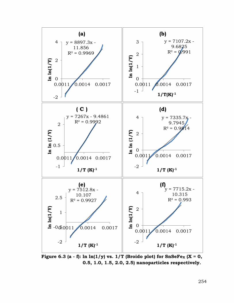
6.3.2 Evaluation of Thermal Parameters of SnSeFeX (X = 0, 0.5,
1.0, 1.5, 2.0, 2.5) Nanoparticles
Broido and C - R thermodynamical method / model have been
used for evaluation of thermal parameters. As described earlier, values of
‘y’ were determined at different temperature interval from TG curve.
These thermal parameters of all SnSeFeX (X = 0, 0.5, 1.0, 1.5, 2.0, 2.5)
nanoparticles can be achieved by ploting ln ln (1/y) versus 1/ T graph,
for major degradation events where significant weight or mass loss is
found. Figure 6.3 (a - f) show the Broido plot (i.e plot of ln ln (1/y) versus
1/ T) for SnSeFeX (X = 0, 0.5, 1.0, 1.5, 2.0, 2.5) nanoparticles
respectively. The slope obtained from these plots, equal to – Ea/ 2.303 R
[8]. Thus, by obtaining value of energy of activation using Equation 6.11,
Equation 6.12 and Equation 6.13 one can easily evaluate the entropy of
activation (ΔS), enthalpy of activation (ΔH) and Gibbs free energy (ΔG)
respectively for pure SnSe nanoparticles.
Similarly of ln[-(1-y)/T2] versus 1 / T graph, have been plotted for
all these pure and iron doped SnSe nanoparticles samples (i.e. in C- R
Temp Cel600.0500.0400.0300.0200.0100.0
DT
A u
V
0.00
-2.00
-4.00
-6.00
-8.00
-10.00
-12.00
-14.00
TG
mg
5.000
4.500
4.000
3.500
3.000
DT
G u
g/m
in100.0
90.0
80.0
70.0
60.0
50.0
40.0
30.0
20.0
10.0

252
method). Figure 6.4 (a) to (f) show the C - R plot for SnSe nanoparticles
doped by 0, 0.05, 0.1, 0.15, 2.0 and 2.5 iron concentration level
respectively. By repeating the process as that for the Broido method,
author has reported all the mentioned thermal parameters for all SnSe
nanoparticles sample.
Thermal parameters of SnSe nanoparticles doped by 0, 0.05, 0.1,
0.15, 2.0 and 2.5 iron concentration level obtained from Broido and
Coats- Redfern (C - R) model have been mentioned in Table 6.2. As the
doping level of iron concentration in SnSe nanoparticles increases (i. e. 0,
0.05, 0.1, 0.15, 2.0 and 2.5), energy of activation first decreases as
73.97, 59.09 and from 0.05, 0.1, 0.15, 2.0 and 2.5 iron concentration it
increase to 64.14 kJ/ mol shown in table 6.2. Similarly ΔS and ΔH
changes by changing the iron concentration level in SnSe nanoparticles.
This can be understand that as we are increasing the doping level of
copper concentration in SnSe nanoparticle, crystallite size or particle size
of SnSe nanoparticles is reduced. This crystallite size or particle size of
as synthesized iron doped SnSe nanoparticles has been calculated from
X- ray diffraction technique, Transmission electron microscopy and UV-
VIS- NIR Spectroscopy (i. e. chapter 3 and chapter 4). It should be noted
that thermal parameters (activation energy, frequency factor, entropy
(ΔS), enthalpy (ΔH) and Gibbs mean free energy (ΔG)) presented here had
been investigated using Broido model.
For this SnSe particles (not nanoparticles) sample, synthesized by
ball milling technique with particle size 200 nm to 500 nm, energy of
activation is found to be 89 kJ/ mol. This value matches to activation
energy obtained for as synthesized iron doped SnSe nanoparticle in this
investigation by using aqueous solution technique [9].
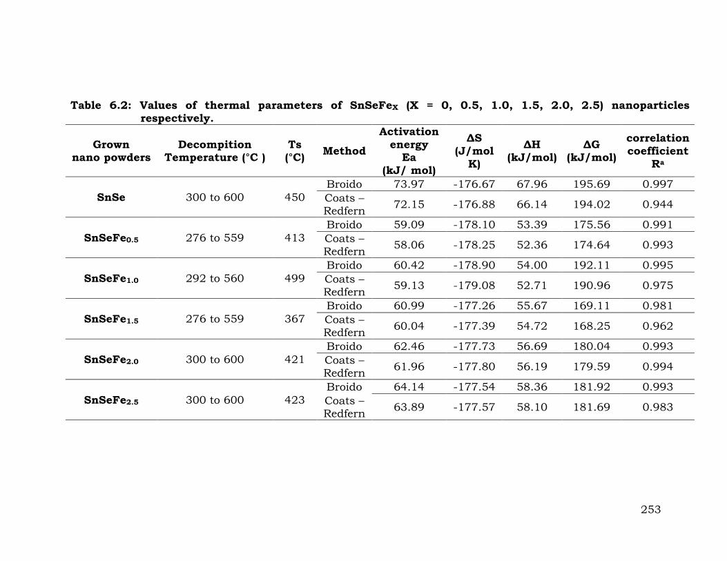
253
Table 6.2: Values of thermal parameters of SnSeFeX (X = 0, 0.5, 1.0, 1.5, 2.0, 2.5) nanoparticles
respectively.
Grown nano powders
Decompition Temperature (°C )
Ts (°C)
Method
Activation energy
Ea
(kJ/ mol)
ΔS
(J/mol
K)
ΔH (kJ/mol)
ΔG (kJ/mol)
correlation
coefficient
Ra
SnSe 300 to 600 450
Broido 73.97 -176.67 67.96 195.69 0.997
Coats – Redfern
72.15 -176.88 66.14 194.02 0.944
SnSeFe0.5 276 to 559 413
Broido 59.09 -178.10 53.39 175.56 0.991
Coats – Redfern
58.06 -178.25 52.36 174.64 0.993
SnSeFe1.0 292 to 560 499
Broido 60.42 -178.90 54.00 192.11 0.995
Coats – Redfern
59.13 -179.08 52.71 190.96 0.975
SnSeFe1.5 276 to 559 367
Broido 60.99 -177.26 55.67 169.11 0.981
Coats – Redfern
60.04 -177.39 54.72 168.25 0.962
SnSeFe2.0 300 to 600 421
Broido 62.46 -177.73 56.69 180.04 0.993
Coats – Redfern
61.96 -177.80 56.19 179.59 0.994
SnSeFe2.5 300 to 600 423
Broido 64.14 -177.54 58.36 181.92 0.993
Coats – Redfern
63.89 -177.57 58.10 181.69 0.983
254
Figure 6.3 (a - f): ln ln(1/y) vs. 1/T (Broido plot) for SnSeFeX (X = 0,
0.5, 1.0, 1.5, 2.0, 2.5) nanoparticles respectively.
y = 8897.3x - 11.856
R² = 0.9969
-2
0
2
4
0.0011 0.0014 0.0017
ln ln(1
/Y
)
(a)
y = 7107.2x - 9.6825
R² = 0.991
-1
0
1
2
3
0.0011 0.0014 0.0017
ln ln(1
/Y
)
1/T(K)-1
(b)
y = 7267x - 9.4861 R² = 0.9992
-1
0.5
2
0.0011 0.0014 0.0017
ln ln
(1/Y
)
1/T (K)-1
( C )
y = 7335.7x - 9.7945
R² = 0.9814
-2
0
2
4
0.0011 0.0014 0.0017
ln ln
(1/Y
)
1/T (K)-1
(d)
y = 7512.8x - 10.107
R² = 0.9927
-2
-0.5
1
2.5
0.0011 0.0014 0.0017 ln ln
(1/Y
)
1/T (K)-1
(e) y = 7715.2x -
10.315 R² = 0.993
-2
0
2
4
0.0011 0.0014 0.0017
ln ln
(1/Y
)
1/T (K)-1
(f)

255
Figure 6.4 (a - f): ln[-ln(1-y)/T2] vs. 1/T (C–R plot) for SnSeFeX (X = 0,
0.5, 1.0, 1.5, 2.0, 2.5) nanoparticles respectively.
y = -8678.3x + 25.792
R² = 0.9443
11
14
17
0.0011 0.0014 0.0017
ln [-l
n(1
-y)/
T2]
1/T (K)-1
(a) y = -6984x +
23.483 R² = 0.9925
11
13
15
0.0012 0.0015 0.0018
ln [-l
n(1
-y)/
T2]
1/T (K)-1
(b)
y = -7112.1x + 23.341
R² = 0.9746
11
13
15
0.0011 0.0014 0.0017
ln [-l
n(1
-y)/
T2]
1/T (K)-1
( c ) y = -7221.1x +
23.789 R² = 0.962
11
14
17
0.0011 0.0014 0.0017
ln [-l
n(1
-y)/
T2]
1/T (K)-1
(d)
y = -7452.8x + 24.034
R² = 0.9941
11
13
15
0.0012 0.0014 0.0016
ln [-l
n(1
-y)/
T2]
1/T (K)-1
(e)
y = -7684.6x + 24.335
R² = 0.9829
11
13
15
0.0012 0.0014 0.0016
ln [-l
n(1
-y)/
T2]
1/T (K)-1
(f)
256
6.3.3 TG & DTA Analysis of SnSeFeX (X = 0, 0.5, 1.0, 1.5, 2.0, 2.5)
Nanoparticles
The SnSeFeX (X = 0, 0.5, 1.0, 1.5, 2.0, 2.5) nanoparticles
synthesized by aqueous solution technique has been subjected to
thermal analysis to study the effect of rise in temperature from room
temperature to 900 °C with a heating rate of 10 K/ min on the weight
loss (TG) and heat flow (DTA). Figure 6.2 (a - f) shows the TG and DTA
curves in air of pure and iron doped SnSe nanoparticles. TG curve of this
sample shows continuous weight losses from room temperature to about
900 °C
The iron (Fe) ion introduces more packing efficiency to the host,
which in turn influences the thermal properties of the material/ host.
The aim of the present work was to study the thermal properties of pure
SnSe and copper doped SnSe nanoparticles using thermogravimetric
analysis and differential scanning calorimetry (TG/ DTA and DSC) [10].
The TG and DTA curves in air of SnSe nanoparticles doped
by 0, 0.5, 1.0, 1.5, 2.0 and 2.5 iron concentration level have been shown
in Figure 6.2 (a - f) [9]. Thermogrammes of all these iron doped
nanoparticles show almost same mass loss events as that of pure or
undoped SnSe nanoparticles.
The results obtained of weight loss from the TGA curve observed
for SnSe nanoparticles doped by 0, 0.5, 1.0, 1.5, 2.0 and 2.5 iron
concentration is tabulated in Table 6.3.
The TG curve exhibits three stages of weight loss: the first one is
less than 12 % occurring from room temperature 35 °C to 275 °C. This
weight loss is described to the removal of water molecules at below 100
°C from the pure and iron doped SnSe nanoparticles sample. The first
weight loss change at low temperatures (i. e. stage I) is due to release of
water/ethanol mixture left in the nanoparticles sample. Although the

257
nanoparticles powder was dried at 100 °C temperature in oven, solvent
molecules from the precipitation procedure remain entrapped in the
nanoparticles. Up to approximately 10 % of the total powder weight could
be lost in this step.
Table 6.3: TG and DTA analysis of SnSeFeX (X = 0, 0.5, 1.0, 1.5, 2.0,
2.5) nanoparticles respectively.
Grown Nano Powders DTG Peak(°c) Weight Loss (%)
SnSe
85 6.2
319 43.6 450
581 5.7
SnSeFe0.5
76.9 8.3
354.1
36.2 413.2
507
657.8 7.7
SnSeFe1.0
98 8
350.9
38.8 414.6
499
668 6.5
SnSeFe1.5
95.2 9.5
323.2
38.3 354
367.8
521.8 2.8
SnSeFe2.0
99 11.25
421 36.83
501
SnSeFe2.5
96 12.18
378
39.45 423
497
The second stage of TGA curve shows weight loss about 40 %
appearing between 275 to 600 °C. There was major change with
compared to other weight loss stages in the weight loss. It indicated that

258
these SnSe nanoparticles synthesized at 200 °C remains almost stable
within the said temperature range in comparison with other weight loss
stages.
The second weight loss is about 40 % between 275 to 600 °C. it is
due to melting of excess Sn and Se in SnSe nanoparticles because Sn
and Se particles starts to melt at about 232 and 221 °C temperature.
Within this temperature range there is not any possibility of melting of
iron, because iron starts to melt about 1535 °C temperature.
The final weight loss is more than 8 % and is between 600 to 900
°C.
Another reason for this is that the stability of SnSe in bulk form is
up to 860 °C temperature because it starts to melt about this
temperature. So it should be noticed that in DTA pattern temperature
below 860 °C, one cannot get any DTA peak due to the melting or
decomposition of SnSe nanoparticles.
The final weight loss is more than 8 % and is between 600 and
about 900 °C. The maximum second stage of the TGA weight loss which
is about 40 % correspondingly, the DTA curve shows peaks at around
400 to 450 °C. X- ray powder diffraction indicates that SnSe
nanoparticles synthesized at 400 °C temperature, does not indicate any
extra reflection peak which proves that these nanoparticles/ compound
is stable up to this temperature. Another reason for this is that the
stability of SnSe in bulk form is up to 861 °C temperature because it
starts to melt about this temperature. So it should be noticed that in
DTA pattern temperature about 400 to 450 °C, one cannot get any DTA
peak due to the melting or decomposition of SnSe nanoparticles. It
should be noted that TG/ DTA of pure SnSe nanoparticles were
performed from room temperature to 900 °C. but here for iron doped
SnSe nanoparticles, For 0, 0.5, 1.0, 1.5, 2.0 and 2.5 iron doping in SnSe

259
nanoparticles, due to less dopant concentration level melting point of
iron doped SnSe nanoparticles could not vary/ changed so much from
that of bulk SnSe compound/ material. DTA curve of this nanoparticles
sample does not show any peak around 860 °C temperature. Around this
temperature in DTA show peak around 550 to 670 °C temperature. When
SnSe has been studied in nanoparticle form, the melting temperature
takes place at other temperature. This change in melting temperature
can be explained on the basis of the large amount of free energy
associated with the grain boundaries of nanoparticles. As material‟s form
has been changed (bulk or nanoparticle) melting point of material has
been changed or by specifically found that in most of the materials
melting point decreases as particle size or crystallite size decrease. Lots
of research on thermal (particularly melting process) characterization
had been done on Sn material. Such type of report on other
semiconductor nanoparticles or group IV - VI compound has not found.
Till today according to our knowledge, thermal characterization of
pure SnSe nanoparticles has not reported or rare publications are found
on the thermal characteristics of nanoparticle semiconductors yet. Hence
author has compared obtained results of the variation in thermal
properties of as synthesized nanoparticles have been compared with
earlier report on the thermal properties of elemental nanopartiecles.
In one report of determination of particle size distribution of the
four kinds of Sn nanoparticles has been presented [11]. The data were
fitted with a Gaussian model, and the average particle diameters were
around 82 nm, 39 nm, 36 nm, and 34 nm, respectively. The DSC curves
of the as- synthesized Sn nanoparticles has been presented. The Sn
nanoparticles synthesized in the presence of 0, 0.1, 0.2 and 0.4 g
surfactants were marked as Sn1, Sn2, Sn3 and Sn4, respectively. The
melting temperatures of the Sn1, Sn2, Sn3 and Sn4 nanoparticles were
260
226.1, 221.8, 221.1 and 219.5 °C, and the corresponding latent heats ΔH
of fusion were 35.9, 23.5, 20.1 and 15.6 J/g, respectively [11].
Lots of research on thermal (particularly melting process)
characterization had been done on Sn material. Such type of report on
other semiconductor nanoparticles or group IV- VI compound has not
found. Up to the 1980s, experimental investigations of the size effect on
melting has been performed in a large variety of simple elements of which
the melting point is relatively low, such as Sn, In, Pb, Ge, Bi, Al, Ag, Cu
and Na. Generally, despite the experimental errors in determining the
melting temperature and particle size, evident melting point depression
was observed for small particles, especially when the particle radius is
below 10 nm [12]. In most cases, an approximately linear relationship
between the melting point and the reciprocal particle size is obtained.
The experimental data falls between the lower and upper limits of the
size dependent melting temperature. It is also noted that defects in the
particles, such as dislocations, stacking faults and grain boundaries
and/or twin boundaries may have considerable effects on the size
dependence of melting point, which is believed to be one of the reasons
accounting for scattering of experimental data [13].
It is now known that the thermal characteristics of all low
dimensional crystals, including metals [14 - 18], semiconductors [19, 20]
and organic crystals [21, 22], depends on their sizes. Although there are
relatively extensive investigations on the size dependent melting of
nanocrystals, it has not been accompanied by the necessary investigation
of the size dependent thermodynamics of nanocrystals [14 - 16, 21, 23,
24]. Such an investigation should deepen our understanding of the size
effect of melting. In particular, a complete understanding of the melting
transition in nanocrystals cannot be obtained without a clear
understanding of enthalpy and entropy of melting, which are important
properties of melting. A physical model presented in [25, 26] for the size
261
dependent enthalpy and entropy based on Mott's expression for the
vibrational entropy of melting for metallic crystals at melting temperature
and a model for the size dependent melting [14 - 18]. The theoretical
prediction of the model for the size dependent melting enthalpy and
entropy has been found to be consistent with experimental evidences on
the metallic nanocrystals of Sn and Al, and the organic nanocrystals of
benzene, chlorobenzene, heptane and naphthalene.
In the vibrational entropy of melting of a bulk crystal, has been
represented by Mott [25], and from the bulk, the maximum phonon
wavelength is truncated by the crystallite size and the surface region has
enhanced configurational enthalpy and entropy. With decreasing
crystallite size the relative significance of all these effects increases. They
represented the variation of enthalpy and entropy of melting as a
function of crystallite size by formally extending Mott’s estimation of the
melting entropy of an infinite metallic crystal to metallic and organic
crystals of finite size and by using an expression for the size dependant
melting temperature. Reasonable agreement between the model
prediction and the experimental data of melting enthalpy and entropy for
nanocrystals of metallic Sn and Al and organic benzene, chlorobenzene,
hepten and naphthalene has been found.
6.4 Conclusion
In this chapter author has explained stage wise weight loss events
carried out from TG / DTA set up SnSe nanoparticles doped by iron at
0, 0.5, 1.0, 1.5, 2.0 and 2.5 concentrations.
Effect of synthesis doping of copper concentration level in iron doped
SnSe nanoparticles on different mass loss / weight loss event have
been represented and explained. Similar effect on the DTA peak
262
position has been presented for pure and copper doped SnSe
nanoparticles.
Author has evaluated thermal parameters i.e. energy of activation Ea,
entropy of activation ΔS, enthalpy of activation ΔH and Gibbs free
energy ΔG by using Broido and Coats – Redfern (C- R) model for all
the aqueous solution technique’s as synthesized pure and iron doped
SnSe nanoparticles. Similarly effect of doping of iron concentration
level in SnSe nanoparticles on all the as mentioned thermal
parameters for iron doped SnSe nanoparticles has been investigated.
The current most challenging tasks in research and developments are
property characterization and device fabrication. Here author
successfully investigated and represented size dependent controls of
thermal parameters / thermal characteristics of nanoparticles. There
are the key steps in the development of nanoscience and
nanotechnology: materials preparation, property characterization and
device fabrication.
References
1. Bernhard Wunderlich, ʻThermal Analysis of Polymeric Materialsʼ, Springer-Verlag Berlin Heidelberg, USA, (2005) 76.
2. A. W. Coats and J. P. Redfern, Thermogravimetric Analysis: A Review, 88 (1963) 906–924.
3. M. E. Brown, ʻIntroduction to Thermal Analysis Technique and Applicationsʼ, Chapman & Hall - New York, (1988).
4. S. M. Mostashari, Y. Kamali Nia & F. Fayyaz, J. Them. Anal. Cal., 91 (1) (2008) 237.
5. A. Broido J. Polym. Sci., 7 (1969) 1761.
6. A. W. Coats and J. P. Redfern,

263
Nature, 201 (4914) (1964) 68.
7. H. H. Horowitz and G. Metzger, Anal. Chem., 35 (1963) 1464.
8. Y. Tonbul, K and Yurdakoc,
Turk. J. Chem., 25 (2001) 333.
9. A. Marcela, R. Aleksander, F. Martin and B. Peter, Acta Montanistica Slovaca Ročník, 16 (2011) 123.
10. C. Linga Raju, J. L. Rao, B. C. V. Reddy and K. Veera. Brahmam, Bull. Mater. Sci., 30 (3) (2007) 215.
11. Z. Chang Dong, G. Yu Lai, Y. Bin and Z. Qijie, Trans. Nonferrous Met. Soc. China, 20 (2010) 248.
12. P. Buffat and J. P. Borel, Phys. Rev. A., 13 (1976) 2287.
13. S. J. Peppiatt and J. R. Sambles, Proc. Roy. Soc. London., A 345 (1975) 387.
14. M. Hasegawa, K. Hoshino and M. Watabe, J. Phys., F 10 (1980) 619.
15. Q. Jiang and F. G. Shi, J. Mater, Sci. Technol., 14 (1998) 171.
16. Q. Jiang, H. Y. Tong, D. T. Hsu, K. Okuyama and F. G. Shi, Thin Solid Film, 312 (1998) 357.
17. Q. Jiang, N. Aya and F. G. Shi, Appl. Phys. A 64 (1997) 627.
18. F. G. Shi J. Mater. Res., 9 (1994) 1307.
19. A. N. Goldstein, C. M. Ether and A. P. Alivisatos, Science., 256 (1992) 1425.
20. A. N. Goldstein, Appl. Phys., A 62 (1996) 33.
21. C. L. Jackson and G. B. Mc Kenna, J. Chem. Phys., 93 (1990) 9002.

264
22. C. L. Jackson and G. B. Mc Kenna,
Chem. Mater., 8 (1996) 2128.
23. S. L. Lai, J. Y. Guo, V. Petrova, G. Ramanath and L. H. Allen, Phys. Rev. Lett., 77 (1996) 99.
24. J. Eckert, J. C. Holzer, C. C. Ahn, Z. Fu and W. L. Johnson, Nanostruct. Mater., 2 (1993) 407.
25. N. F. Mott, Proc. Roy. Soc., A 146 (1934) 465.
26. A. R. Regel and V. M. Glazov, Semiconductors, 29 (1995) 405.