Chapter 6 SUPER-CONVERGENT PATCH RECOVERY · PDF fileChapter 6 SUPER-CONVERGENT PATCH RECOVERY...

Chapter 6

SUPER-CONVERGENTPATCH RECOVERY

6.1 Patch Implementation Datebase

Since the super-convergent patch (SCP) recovery method is relativity easy tounderstand and is accurate for a wide range of problems, it was selected forimplementation in the educational programMODEL. Its implementation is designed foruse with most of the numerically integrated 1-D, 2-D, and 3-D elements in theMODELlibrary. Most of the literature on the SCP recovery methods are limited to a singleelement type and a single patch type. The present version is somewhat more general inallowing a mixture of element shapes in the mesh and a mesh that is either linear,quadratic, or cubic in its polynomial degree.

This represents actually the third version of the SCP algorithm and is asimplification of the first two. The method given here was originally developed for ap-adaptive code where all the elements could have a different polynomial degree on eachelement edge. That version was then extended to an object-oriented F90p-adaptiveprogram that also included equilibrium error contributions as suggested by Wiberg [12]and others. Including thep-adaptive features and the object-oriented features made thedata base more complicated and required more planning and programming than desirablein an introductory text such as this one. However, the version given here has shown to berobust and useful.

The SCP recovery process is clearly heuristic in nature, so some arbitrary choicesneed to be made in the implementation. We begin try defining a "patch" to be a localgroup of elements surrounding at least one interior node or being adjacent to a boundarynode. The original research in SCP recovery methods used patches sequentially builtaround each node in the mesh. Later it was widely recognized that one could use a patchfor every element in the mesh. Therefore, three types of patches will be defined here:1. Node-based patch: An adjacent group of elements associated with a particular node.2. Element-based patch: All elements adjacent to a particular element.3. Face-based patch: This subset of the element-based patch includes only the adjacent

elements that share a common face with the selected element. For two-dimensional

4.3 Draft− 5/27/04 © 2004 J.E. Akin 145

146 J. E. Akin

elements this means that they share a common edge.Those three choices for patches were shown in Fig. 12.2.2. Any of these three

definitions of a patch requires that one have a mesh "neighbors list". That is, we willneed a list of elements adjacent to each node, or a list of elements adjacent to eachelement, or the subset list of facing element neighbors. These can be expensive lists tocreate, but are often needed for other purposes and are sometime supplied by a meshgeneration code or an equation re-ordering program.

Here several routines are included for creating the lists and printing them.Normally, since those neighbor lists are of unknown variable lengths, they would bestored in a linked list data structure. Here, for simplicity, they hav e been placed inrectangular arrays and padded with trailing zeros. This wastes a little storage space butkeeps the general code simpler. Sev eral of these routines are actually invoked at the meshinput stage as part of the data checking process. The neighbor lists are usually quite largeand are not usually listed but can be (via keywordslist_el_to_el or pt_el_list).

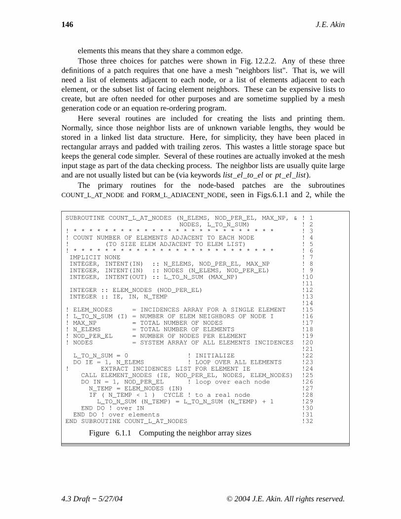
The primary routines for the node-based patches are the subroutinesCOUNT_L_AT_NODE and FORM_L_ADJACENT_NODE, seen in Figs.6.1.1 and 2, while the

SUBROUTINE COUNT_L_AT_NODES (N_ELEMS, NOD_PER_EL, MAX_NP, & ! 1NODES, L_TO_N_SUM) ! 2

! * * * * * * * * * * * * * * * * * * * * * * * * * * ! 3! COUNT NUMBER OF ELEMENTS ADJACENT TO EACH NODE ! 4! (TO SIZE ELEM ADJACENT TO ELEM LIST) ! 5! * * * * * * * * * * * * * * * * * * * * * * * * * * ! 6

IMPLICIT NONE ! 7INTEGER, INTENT(IN) :: N_ELEMS, NOD_PER_EL, MAX_NP ! 8INTEGER, INTENT(IN) :: NODES (N_ELEMS, NOD_PER_EL) ! 9INTEGER, INTENT(OUT) :: L_TO_N_SUM (MAX_NP) !10

!11INTEGER :: ELEM_NODES (NOD_PER_EL) !12INTEGER :: IE, IN, N_TEMP !13

!14! ELEM_NODES = INCIDENCES ARRAY FOR A SINGLE ELEMENT !15! L_TO_N_SUM (I) = NUMBER OF ELEM NEIGHBORS OF NODE I !16! MAX_NP = TOTAL NUMBER OF NODES !17! N_ELEMS = TOTAL NUMBER OF ELEMENTS !18! NOD_PER_EL = NUMBER OF NODES PER ELEMENT !19! NODES = SYSTEM ARRAY OF ALL ELEMENTS INCIDENCES !20

!21L_TO_N_SUM = 0 ! INITIALIZE !22DO IE = 1, N_ELEMS ! LOOP OVER ALL ELEMENTS !23

! EXTRACT INCIDENCES LIST FOR ELEMENT IE !24CALL ELEMENT_NODES (IE, NOD_PER_EL, NODES, ELEM_NODES) !25DO IN = 1, NOD_PER_EL ! loop over each node !26

N_TEMP = ELEM_NODES (IN) !27IF ( N_TEMP < 1 ) CYCLE ! to a real node !28

L_TO_N_SUM (N_TEMP) = L_TO_N_SUM (N_TEMP) + 1 !29END DO ! over IN !30

END DO ! over elements !31END SUBROUTINE COUNT_L_AT_NODES !32

Figure 6.1.1 Computing the neighbor array sizes

4.3 Draft− 5/27/04 © 2004 J.E. Akin. All rights reserved.

Finite Elements, SCP Recovery 147

SUBROUTINE FORM_L_ADJACENT_NODES (N_ELEMS, NOD_PER_EL, MAX_NP, & ! 1NODES, NEIGH_N, L_TO_N_NEIGH) ! 2

! * * * * * * * * * * * * * * * * * * * * * * * * * * * * * * ! 3! TABULATE ELEMENTS ADJACENT TO EACH NODE ! 4! (TO SIZE ELEM ADJACENT TO ELEM LIST) ! 5! * * * * * * * * * * * * * * * * * * * * * * * * * * * * * * ! 6IMPLICIT NONE ! 7

INTEGER, INTENT(IN) :: N_ELEMS, NOD_PER_EL, MAX_NP, NEIGH_N ! 8INTEGER, INTENT(IN) :: NODES (N_ELEMS, NOD_PER_EL) ! 9INTEGER, INTENT(OUT) :: L_TO_N_NEIGH (NEIGH_N, MAX_NP) !10

!11INTEGER :: ELEM_NODES (NOD_PER_EL), COUNT (MAX_NP) ! scratch !12INTEGER :: IE, IN, N_TEMP !13

!14! ELEM_NODES = INCIDENCES ARRAY FOR A SINGLE ELEMENT !15! L_TO_N_SUM (I) = NUMBER OF ELEM NEIGHBORS OF NODE I !16! MAX_NP = TOTAL NUMBER OF NODES !17! N_ELEMS = TOTAL NUMBER OF ELEMENTS !18! NOD_PER_EL = NUMBER OF NODES PER ELEMENT !19! NODES = SYSTEM ARRAY OF INCIDENCES OF ALL ELEMENTS !20

!21L_TO_N_NEIGH = 0 ; COUNT = 0 ! INITIALIZE !22DO IE = 1, N_ELEMS ! LOOP OVER ALL ELEMENTS !23

!24! EXTRACT INCIDENCES LIST FOR ELEMENT IE !25

CALL ELEMENT_NODES (IE, NOD_PER_EL, NODES, ELEM_NODES) !26!27

DO IN = 1, NOD_PER_EL ! loop over each node !28N_TEMP = ELEM_NODES (IN) !29IF ( N_TEMP < 1 ) CYCLE ! to a real node !30

COUNT (N_TEMP) = COUNT (N_TEMP) + 1 !31L_TO_N_NEIGH (COUNT (N_TEMP), N_TEMP) = IE !32

END DO ! over IN nodes !33END DO ! over elements !34

END SUBROUTINE FORM_L_ADJACENT_NOD !35

Figure 6.1.2 Find elements at every node

element-based patches use the two similar subroutinesCOUNT_ELEMS_AT_ELEM andFORM_ELEMS_AT_ELwhich are given in Figs. 6.1.3 and 4. These routines are also usefulin validating meshes that have been prepared by hand. Building lists of neighbors cantake a lot of processing but they useful in plotting and post-processing.

In MODEL the default is to use an element-based patch. However, one caninvestigate other options by utilizing some of the available control keywords given in Fig.6.1.5. Having selected a patch type, we should now giv e consideration to the kind of datathat will be needed for the SCP recovery. There are two main segments in the process:1. Averaging the patch and system nodal fluxes.2. Using the system nodal fluxes in the calculation of an error estimate.

The whole basis of the SCP recovery is that there are special locations within anelement where we can show that the derivatives are most accurate or exact for a givenpolynomial degree. We refer to such locations as element super-convergent points. Theyare sometimes calledBarlow points. The derivation of the locations generally shows them


148 J. E. Akin

SUBROUTINE COUNT_ELEMS_AT_ELEM (N_ELEMS, NOD_PER_EL, MAX_NP, & ! 1L_FIRST, L_LAST, NODES, NEEDS, L_TO_L_SUM, N_WARN) ! 2

! * * * * * * * * * * * * * * * * * * * * * * * * * * * * * * ! 3! COUNT NUMBER OF ELEMENTS ADJACENT TO OTHER ELEMENTS ! 4! * * * * * * * * * * * * * * * * * * * * * * * * * * * * * * ! 5IMPLICIT NONE ! 6

INTEGER, INTENT(IN) :: N_ELEMS, NOD_PER_EL, MAX_NP, NEEDS ! 7INTEGER, INTENT(IN) :: L_FIRST (MAX_NP), L_LAST (MAX_NP) ! 8INTEGER, INTENT(IN) :: NODES (N_ELEMS, NOD_PER_EL) ! 9INTEGER, INTENT(OUT) :: L_TO_L_SUM (N_ELEMS) !10INTEGER, INTENT(INOUT) :: N_WARN !11

!12INTEGER :: ELEM_NODES (NOD_PER_EL), NEIG_NODES (NOD_PER_EL) !13INTEGER :: FOUND, IE, IN, L_TEST, L_START, L_STOP, N_TEST !14INTEGER :: NEED, KOUNT, NULLS !15

!16! ELEM_NODES = INCIDENCES ARRAY FOR A SINGLE ELEMENT !17! KOUNT = NUMBER OF COMMON NODES !18! L_FIRST (I) = ELEMENT WHERE NODE I FIRST APPEARS !19! L_LAST (I) = ELEMENT WHERE NODE I LAST APPEARS !20! L_TO_L_SUM (I) = NUMBER OF ELEM NEIGHBORS OF ELEMENT I !21! MAX_NP = TOTAL NUMBER OF NODES !22! NEEDS = NUMBER OF COMMON NODES TO BE A NEIGHBOR !23! N_ELEMS = TOTAL NUMBER OF ELEMENTS !24! NOD_PER_EL = NUMBER OF NODES PER ELEMENT !25! NODES = SYSTEM ARRAY OF INCIDENCES OF ALL ELEMENTS !26

!27L_TO_L_SUM = 0 ; NEED = MAX (1, NEEDS) ! INITIALIZE !28

!29MAIN : DO IE = 1, N_ELEMS ! LOOP OVER ALL ELEMENTS !30

FOUND = 0 ! INITIALIZE !31!32

! EXTRACT INCIDENCES LIST FOR ELEMENT IE !33CALL ELEMENT_NODES (IE, NOD_PER_EL, NODES, ELEM_NODES) !34

!35! ESTABLISH RANGE OF POSSIBLE ELEMENT NEIGHBORS !36

L_START = N_ELEMS ; L_STOP = 0 !37DO IN = 1, NOD_PER_EL !38

N_TEST = ELEM_NODES (IN) !39IF ( N_TEST < 1 ) CYCLE! to a real node !40

L_START = MIN (L_START, L_FIRST (N_TEST) ) !41L_STOP = MAX (L_STOP, L_LAST (N_TEST) ) !42

END DO !43!44

Figure 6.1.3a Interface and data for elements joining element



! LOOP OVER POSSIBLE ELEMENT NEIGHBORS !45IF ( L_START <= L_STOP) THEN !46

RANGE : DO L_TEST = L_START, L_STOP !47IF ( L_TEST /= IE) THEN !48

KOUNT = 0 ! NO COMMON NODES !49!50

! LOOP OVER INCIDENCES OF POSSIBLE ELEMENT NEIGHBOR !51CALL ELEMENT_NODES (L_TEST,NOD_PER_EL,NODES,NEIG_NODES) !52LOCAL : DO IN = 1, NOD_PER_EL !53

N_TEST = NEIG_NODES (IN) !54IF ( N_TEST < 1 .OR. N_TEST > MAX_NP ) THEN !55

PRINT *, ’INVALID NODE ’, N_TEST, ’ AT ’, L_TEST !56N_WARN = N_WARN + 1 ! INCREMENT WARNING !57CYCLE LOCAL ! to a real node !58

END IF ! IMPOSSIBLE NODE !59IF ( L_FIRST (N_TEST) > IE ) CYCLE LOCAL ! to next node !60IF ( L_LAST (N_TEST) < IE ) CYCLE LOCAL ! to next node !61

!62! COMPARE WITH INCIDENCES OF ELEMENT IE !63

IF ( ANY ( ELEM_NODES == N_TEST ) ) THEN !64KOUNT = KOUNT + 1 !65IF ( KOUNT == NEED ) THEN ! IS A NEIGHBOR !66

FOUND = FOUND + 1 !67EXIT LOCAL ! this L_TEST element search loop !68

END IF ! NUMBER NEEDED !69END IF !70

END DO LOCAL ! over in !71END IF !72

END DO RANGE ! over candidate element L_TEST !73END IF ! a possible candidate !74L_TO_L_SUM (IE) = FOUND !75

END DO MAIN ! over all elements !76!77

PRINT *, ’MAXIMUM NUMBER OF ELEMENT NEIGHBORS = ’, & !78MAXVAL (L_TO_L_SUM) !79

NULLS = COUNT ( L_TO_L_SUM == 0 ) ! CHECK DATA !80IF ( NULLS > 0 ) THEN !81

PRINT *, ’WARNING, ’, NULLS, ’ ELEMENTS HAVE NO NEIGHBORS’ !82N_WARN = N_WARN + 1 ! INCREMENT WARNING !83

END IF !84END SUBROUTINE COUNT_ELEMS_AT_ELEM !85

Figure 6.1.3b Fill the neighbor array and validate


150 J. E. Akin

SUBROUTINE FORM_ELEMS_AT_EL (N_ELEMS, NOD_PER_EL, MAX_NP, & ! 1L_FIRST, L_LAST, NODES, N_SPACE, & ! 2L_TO_L_SUM, L_TO_L_NEIGH, & ! 3NEIGH_L, NEEDS, ON_BOUNDARY) ! 4

! * * * * * * * * * * * * * * * * * * * * * * * * * * * * * ! 5! FORM LIST OF ELEMENTS ADJACENT TO OTHER ELEMENTS ! 6! * * * * * * * * * * * * * * * * * * * * * * * * * * * * * ! 7

IMPLICIT NONE ! 8INTEGER, INTENT(IN) :: N_ELEMS, NOD_PER_EL, MAX_NP, NEIGH_L ! 9INTEGER, INTENT(IN) :: L_FIRST (MAX_NP), L_LAST (MAX_NP) ! 10INTEGER, INTENT(IN) :: NODES (N_ELEMS, NOD_PER_EL) ! 11INTEGER, INTENT(IN) :: L_TO_L_SUM (N_ELEMS) ! 12INTEGER, INTENT(IN) :: N_SPACE, NEEDS ! for pt, edge, face ! 13INTEGER, INTENT(OUT) :: L_TO_L_NEIGH (NEIGH_L, N_ELEMS) ! 14LOGICAL, INTENT(INOUT) :: ON_BOUNDARY (N_ELEMS) ! 15

! 16INTEGER :: ELEM_NODES (NOD_PER_EL), NEIG_NODES (NOD_PER_EL) ! 17INTEGER :: IE, IN, L_TEST, L_START, L_STOP, N_TEST ! 18INTEGER :: FOUND, NEXT, SUM_L_TO_L ! 19INTEGER :: IO_1, KOUNT, NEED, N_FACES, WHERE ! 20

! 21! ON_BOUNDARY = TRUE IF ELEMENT HAS A FACE ON BOUNDARY ! 22! ELEM_NODES = INCIDENCES ARRAY FOR A SINGLE ELEMENT ! 23! FOUND = CURRENT NUMBER OF LOCAL NEIGHBORS ! 24! KOUNT = CURRENT NUMBER OF COMMON NODES ! 25! L_FIRST (I) = ELEMENT WHERE NODE I FIRST APPEARS ! 26! L_LAST (I) = ELEMENT WHERE NODE I LAST APPEARS ! 27! L_TO_L_NEIGH = ELEM NEIGHBOR J OF ELEMENT I ! 28! L_TO_L_SUM = NUMBER OF ELEM NEIGHBORS OF ELEMENT I ! 29! NEEDS = NUMBER OF COMMON NODES TO BE A NEIGHBOR ! 30! NEIGH_L = MAXIMUM NUMBER OF NEIGHBORS AT A ELEMENT ! 31! MAX_NP = TOTAL NUMBER OF NODES ! 32! N_ELEMS = TOTAL NUMBER OF ELEMENTS ! 33! NOD_PER_EL = NUMBER OF NODES PER ELEMENT ! 34! NODES = SYSTEM ARRAY OF INCIDENCES OF ELEMENTS ! 35! WHERE = LOCATION TO INSERT NEIGHBOR, <= MAX_FACES ! 36

! 37NEED = MAX (1, NEEDS) ; L_TO_L_NEIGH = 0 ! INITIALIZE ! 38MAIN : DO IE = 1, N_ELEMS ! ELEMENT LOOP ! 39

! 40SUM_L_TO_L = L_TO_L_SUM (IE) ! MAX NEIGHBORS ! 41FOUND = COUNT (L_TO_L_NEIGH (:, IE) > 0) ! PREVIOUSLY FOUND ! 42IF ( FOUND == SUM_L_TO_L ) CYCLE MAIN ! ALL FOUND ! 43

! 44! EXTRACT INCIDENCES LIST FOR ELEMENT IE ! 45

CALL ELEMENT_NODES (IE, NOD_PER_EL, NODES, ELEM_NODES) ! 46! 47

! ESTABLISH RANGE OF POSSIBLE ELEMENT NEIGHBORS ! 48L_START = N_ELEMS + 1 ; L_STOP = 0 ! 49DO IN = 1, NOD_PER_EL ! 50

L_START = MIN (L_START, L_FIRST (ELEM_NODES (IN)) ) ! 51L_STOP = MAX (L_STOP, L_LAST (ELEM_NODES (IN)) ) ! 52

END DO ! 53L_START = MAX (L_START, IE+1) ! SEARCH ABOVE IE ONLY ! 54

! 55

Figure 6.1.4a Interface and data for element neighbors



! LOOP OVER POSSIBLE ELEMENT NEIGHBORS ! 56IF ( L_START <= L_STOP) THEN ! 57

RANGE : DO L_TEST = L_START, L_STOP ! 58KOUNT = 0 ! NO COMMON NODES ! 59

! 60! EXTRACT NODES OF L_TEST ! 61

CALL ELEMENT_NODES (L_TEST,NOD_PER_EL,NODES,NEIG_NODES) ! 62! 63

! LOOP OVER INCIDENCES OF POSSIBLE ELEMENT NEIGHBOR ! 64LOCAL : DO IN = 1, NOD_PER_EL ! 65

N_TEST = NEIG_NODES (IN) ! 66IF ( N_TEST < 1 ) CYCLE ! to a real node ! 67IF (L_FIRST (N_TEST) > IE) CYCLE LOCAL ! to next node ! 68IF (L_LAST (N_TEST) < IE) CYCLE LOCAL ! to next node ! 69

! 70! COMPARE WITH INCIDENCES OF ELEMENT IE ! 71

IF ( ANY ( ELEM_NODES == N_TEST ) ) THEN ! 72KOUNT = KOUNT + 1 ! SHARED NODE COUNT ! 73IF ( KOUNT == NEED ) THEN ! NEIGHBOR PAIR FOUND ! 74

FOUND = FOUND + 1 ! INSERT THE PAIR ! 75! 76

! NOTE: THIS INSERT IS NOT ORDERED. ! 77WHERE = FOUND ! OR ORDER THE CURRENT FACE ! 78L_TO_L_NEIGH (WHERE, IE) = L_TEST ! 1 of 2 ! 79

! 80NEXT = COUNT ( L_TO_L_NEIGH(:, L_TEST) > 0 ) ! 81WHERE = NEXT+1 ! OR ORDER THE NEIGHBOR FACE ! 82

! 83IF ( L_TO_L_SUM (L_TEST) > NEXT ) & ! 84

L_TO_L_NEIGH (NEXT+1, L_TEST) = IE ! 2 of 2 ! 85IF ( SUM_L_TO_L == FOUND ) CYCLE MAIN ! ALL ! 86CYCLE RANGE ! this L_TEST element search loop ! 87

END IF ! NUMBER NEEDED ! 88END IF ! SHARE AT LEAST ONE COMMON NODE ! 89

END DO LOCAL ! over N_TEST ! 90END DO RANGE ! over candidate element L_TEST ! 91

END IF ! a possible candidate ! 92END DO MAIN! over all elements ! 93

! 94IF ( NEED >= N_SPACE ) THEN ! EDGE OR FACE NEIGHBOR DATA ! 95

! SAVE THE ELEMENT NUMBERS THAT FACE THE BOUNDARY ! 96DO IE = 1, N_ELEMS ! 97

CALL GET_LT_FACES (IE, N_FACES) ! 98IF ( N_FACES > 0 ) THEN ! MIGHT BE ON THE BOUNDARY ! 99

IF ( ANY (L_TO_L_NEIGH (1:N_FACES, IE) == 0)) THEN !100ON_BOUNDARY (IE) = .TRUE. !101

END IF ! ON BOUNDARY !102END IF ! POSSIBLE ELEMENT !103

END DO ! OVER ELEMENTS !104END IF ! SEARCH OF FACING NEIGHBORS !105

END SUBROUTINE FORM_ELEMS_AT_EL !106

Figure 6.1.4b Fill the neighbor array and check boundary


152 J. E. Akin

# SCP_WORD TYPICAL_VALUE ! REMARKS [DEFAULT]debug_scp ! Debug the SCP averaging process [F]face_nodes 3 ! Number of shared nodes on an element face [d]grad_base_error ! Base error estimates on gradients only [F]list_el_to_el ! List elements adjacent to elements [F]no_scp_ave ! Do NOT get superconvergent patch averages [F]no_error_est ! Do NOT compute SCP element error estimates [F]pt_el_list ! List all the elements at each node [F]scp_center_only ! Use center node or element only in average [T]scp_center_no ! Use all elements in the patch in average [F]scp_deg_inc 1 ! Increase patch degree by this (1 or 2) [0]scp_max_error 5. ! Allowed % error in energy norm [1]scp_neigh_el ! Element based patch, all neighbors (default) [T]scp_neigh_face ! Element based patch, facing neighbors [F]scp_neigh_pt ! Nodal based patch, all element neighbors [F]scp_not_once ! Scatter a node at each appearance [F]scp_only_once ! Scatter to a node only once per patch [T]scp_2nd_deriv ! Recover 2nd derivatives data also [F]

Figure 6.1.5 Optional SCP control keywords

to coincide with the Gaussian quadrature points (as illustrated here in sections 3.8 and6.5). Here we will assume that the minimum number of quadratic points needed toproperly form the element matrices have locations that correspond to the element super-convergent points, or are reasonably close to them. Thus, as we process each element tobuild its square matrix, we will want to save, at each quadrature point, its physicallocation in space and the differential operator matrix,B, that will allow the accurategradients to be computed from the local nodal solution. Looking ahead to the errorestimation or other post-processing, we know that at times we will also want to have theconstitutive matrix,E, so we will also save it. Note that we are allowing for different, butcompatible, element shapes in the mesh (and patches) and they would require differentintegration rules.

Now we should look ahead to how the above data are to be recovered in the SCPsection of the code. The main observation is that, for an unstructured mesh, the elementnumbers for the elements adjacent to a particular node or element are totally random.While we have a straight-forward way to save the above data in a sequential fashion, weneed to recover the element data in a random fashion. Thus, we either need to build adatabase that allows random access recovery of that sequential information or we mustdecide to re-compute the data in each element of each patch. The author considers thelatter to be too expensive, so we select the new database option. In the examples that arepresented later the reader will note function calls to save these data, but they could beomitted if the user was willing to pay the cost of recomputing the data.

For the database structure to save and recover the data we could select linked lists,or a tree structure, but there is a simpler way. Fortran has always had a feature known asa "direct access" file that allows the user to randomly recover or change data. The actualdata structure employed is left up to the group that writes the compiler, and is mainlyhidden from the user. Howev er, the user must declare the "record number" of the data setto be recovered or changed. Likewise, the record number of each data set must be givenas the data are saved to the random access file. This means that some logical way will be



SUBROUTINE POST_PROCESS_GRADS (NODES, DD, ITER) ! 1! * * * * * * * * * * * * * * * * * * * * * * * * * * * * ! 2! SAVE ELEMENT GRADIENTS AS SCP INPUT RECORDS ! 3! * * * * * * * * * * * * * * * * * * * * * * * * * * * * ! 4Use System_Constants ! for L_S_TOT, N_D_FRE, NOD_PER_EL, ! 5

! N_L_TYPE, N_PRT, THIS_EL, U_FLUX ! 6Use Elem_Type_Data ! for PT (LT_PARM, LT_QP), WT (LT_QP), ! 7

! G (LT_GEOM, LT_QP), DLG (LT_PARM, LT_GEOM, LT_QP), ! 8! H (LT_N), DLH (LT_PARM, LT_N , LT_QP), C (LT_FREE), ! 9! S (LT_FREE, LT_FREE), ELEM_NODES (LT_N), D (LT_FREE) !10

Use Interface_Header ! for GET_ELEM_* !11IMPLICIT NONE !12REAL(DP), INTENT(IN) :: DD (N_D_FRE) !13INTEGER, INTENT(IN) :: NODES (L_S_TOT, NOD_PER_EL), ITER !14INTEGER :: IE, LT ! Loops, element type !15

!16! D = NODAL PARAMETERS ASSOCIATED WITH AN ELEMENT !17! DD = ARRAY OF SYSTEM DEGREES OF FREEDOM !18! INDEX = SYSTEM DOF NOS ASSOCIATED WITH ELEMENT !19! ITER = CURRENT ITERATION NUMBER !20! ELEM_NODES = THE NOD_PER_EL INCIDENCES OF THE ELEMENT !21! NOD_PER_EL = NUMBER OF NODES PER ELEMENT !22! N_D_FRE = TOTAL NUMBER OF SYSTEM DEGREES OF FREEDOM !23! N_L_TYPE = NUMBER OF DIFFERENT ELEMENT TYPES USED !24! N_ELEMS = NUMBER OF ELEMENTS IN SYSTEM !25! NODES = ELEMENT INCIDENCES OF ALL ELEMENTS !26! U_FLUX = BINARY UNIT TO STORE GRADIENTS OR FLUXES !27

!28LT = 1 ! INITIALIZE ELEMENT TYPES !29WRITE (N_PRT, "(/,’BEGIN SCP SAVE, ITER =’, I4)") ITER !30

!31!--> LOOP OVER ELEMENTS !32

DO IE = 1, N_ELEMS ! for elements, boundary segments !33CALL SET_THIS_ELEMENT_NUMBER (IE) ! Set THIS_EL !34

!35! VALIDATE ELEMENT TYPE !36

IF ( N_L_TYPE > 1) LT = L_TYPE (IE) ! GET TYPE !37IF ( LT /= LAST_LT ) THEN ! this is a new type !38

CALL SET_ELEM_TYPE_INFO (LT) ! Set controls !39END IF ! a new element type !40

!41! RECOVER ELEMENT DEGREES OF FREEDOM !42

ELEM_NODES = GET_ELEM_NODES (IE, LT_N, NODES) !43INDEX = GET_ELEM_INDEX (LT_N, ELEM_NODES) !44D = GET_ELEM_DOF (DD) ! Get all nodal dof !45

!46!--> USE DOF TO RECOVER FLUXES, LIST, SAVE FOR SCP !47

IF ( USE_EXACT_FLUX ) THEN !48CALL LIST_ELEM_AND_EXACT_FLUXES (U_FLUX, IE) !49

ELSE !50CALL LIST_ELEM_FLUXES (U_FLUX, IE) !51

END IF ! an exact solution is known !52END DO ! over all elements !53

END SUBROUTINE POST_PROCESS_GRADS !54

Figure 6.1.6 Preparing data for averaging or post-processing


154 J. E. Akin

needed to create a unique number for each record at any quadrature point in the mesh.For a mesh with a single element type and a single integration rule, we could write

a simple equation for the record number. Here we are allowing a mixture of elementtypes and quadrature rules, so we store the record number at each quadrature point in aninteger array sized for the maximum number of elements and the maximum number ofquadrature points per element. The record numbers are created sequentially as theelement matrices are integrated. A file structure,SCP_RECORD_NUMBER, is supplied forrandomly recovering the integer record number at any integration point in any element.Like any other file used in a program, a random access file must be opened. It is openedas aDIRECT access file ofUNFORMATTED, or binary, records to minimize storage.We must also declare the length of the data records. It is actually hardware-dependent, soF90 includes an intrinsic function,INQUIRE(IOLENGTH), that will compute the recordlength given a list of variables and/or arrays to be included in each record. The unitnumber assigned to the random access file holding the SCP records is given the variablename U_SCPR.

As mentioned above the SCP process can be used to determine the average nodalfluxes and to use them to compute the element error estimates. The general outline of theprocess is as follows:1. Preliminary

a. Build a list of element neighbors.b. Open the sequential file unit U_FLUX to receive element data related to flux

calculations. Those data can also be used for optional post-processing.c. Compute the record length necessary to store the coordinates and flux

components at a point.d. Open the random access file unit U_SCPR that will receive the quadrature

point coordinates and flux components.

2. Element Matrices Generation Loopa. For each element save its number of integration points to file unit U_FLUX.b. Within the numerical integration loop of the element sequentially save the

arrays XYZ , E, and B at each point so that the gradients and/or fluxcomponents can be found at the point.

c. When all elements have been processed rewind the file U_FLUX to itsbeginning.

3. Flux Calculations and Saving Them for Averaging

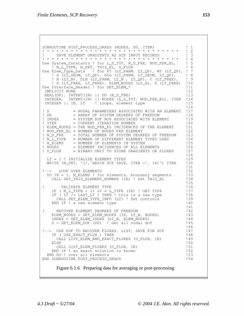
After the solution has been obtained it is possible to compute the flux (and gradient)components within each element so that they can be smoothed to nodal values. Theelement flux calculation is done in subroutinePOST_PROCESS_GRADS, as detailed inFig. 6.1.6. First, the SCP record number is set to zero. Next, each element isprocessed in a loop:a. Recover the element type;b. Gather the nodal degrees of freedom of the element;



SUBROUTINE LIST_ELEM_FLUXES (N_FILE, IE) ! 1! * * * * * * * * * * * * * * * * * * * * * * * * * * * * ! 2! LIST ELEMENT FLUXES AT QUADRATURE POINTS, ON N_FILE ! 3! * * * * * * * * * * * * * * * * * * * * * * * * * * * * ! 4Use System_Constants ! for N_ELEMS, N_R_B, N_SPACE, ! 5

! FLUX_NAME, XYZ_NAME, N_FILE5, IS_ELEMENT, U_PLT4, ! 6! U_SCPR, GRAD_BASE_ERROR ! 7

Use Elem_Type_Data ! for LT_FREE, D (LT_FREE) ! 8IMPLICIT NONE ! 9INTEGER, INTENT(IN) :: N_FILE, IE !10INTEGER, SAVE :: TEST_IE, TEST_IP, J, N_IP, EOF, IO_1 !11REAL(DP), SAVE :: DERIV_MAX = 0.d0 !12

!13! Automatic Arrays !14

REAL(DP) :: XYZ (N_SPACE), E (N_R_B, N_R_B), & !15B (N_R_B, LT_FREE), STRAIN (N_R_B + 2), & !16STRESS (N_R_B + 2) !17

!18! B = GRADIENT VERSUS DOF MATRIX: (N_R_B, LT_FREE) !19! D = NODAL PARAMETERS ASSOCIATED WITH AN ELEMENT !20! E = ELEMENT CONSTITUTIVE MATRIX AT GAUSS POINT !21! LT_N = NUMBER OF NODES PER ELEMENT !22! LT_FREE = NUMBER OF DEGREES OF FREEDOM PER ELEMENT !23! N_ELEMS = TOTAL NUMBER OF ELEMENTS !24! N_R_B = NUMBER OF ROWS IN B AND E MATRICES !25! N_SPACE = DIMENSION OF SPACE !26! N_FILE = UNIT FOR POST SOLUTION MATRICES STORAGE !27! STRAIN = GENERALIZED STRAIN OR FLUX VECTOR !28! STRESS = GENERALIZED STRESS OR GRADIENT VECTOR !29! XYZ = SPACE COORDINATES AT A POINT !30! U_PLT4 = UNIT TO STORE PLOT DATA, IF > 0 !31! U_SCPR = BINARY UNIT FOR SUPER_CONVERGENT PATCH RECOVERY !32

!33!--> FIRST CALL: PRINT TITLES, INITIALIZE, OPEN FILE !34

IF ( IE == 1) THEN ! FIRST ELEMENT !35REWIND (N_FILE) ; RECORD_NUMBER = 0 ! INITIALIZE !36WRITE (N_PRT, 5) XYZ_NAME (1:N_SPACE), FLUX_NAME (1:N_R_B) !375 FORMAT (/, & !38’** FLUX COMPONENTS AT ELEMENT INTEGRATION POINTS **’, & !39/, ’ELEMENT, PT, ’, (6A12) ) !40

!41! OPEN FLUX PLOT FILE IF ACTIVE (BINARY FASTER) !42

IF (N_FILE5 >0) OPEN (N_FILE5,FILE=’el_qp_xyz_grads.tmp’,& !43ACTION=’WRITE’, STATUS=’REPLACE’, IOSTAT = IO_1) !44

IF (U_PLT4 > 0) OPEN (U_PLT4,FILE=’el_qp_xyz_fluxes.tmp’,& !45ACTION=’WRITE’, STATUS=’REPLACE’, IOSTAT = IO_1) !46

END IF ! THIS IS THE FIRST ELEMENT !47!48

Figure 6.1.7a Interface and data to establish SCP records


156 J. E. Akin

! IS THIS AN ELEMENT, BOUNDARY, OR ROBIN SEGMENT ? !49IF ( IS_ELEMENT ) THEN ! ELEMENT RESULTS !50

!51READ (N_FILE, IOSTAT = EOF) N_IP ! # INTEGRATION POINTS !52

!53!--> READ COORDS, CONSTITUTIVE, AND DERIVATIVE MATRIX !54

DO J = 1, N_IP ! OVER ALL INTEGRATION POINTS !55READ (N_FILE, IOSTAT = EOF) XYZ, E, B !56

!57! CALCULATE DERIVATIVES, STRAIN = B * D !58

STRAIN (1:N_R_B) = MATMUL (B, D) !59!60

! FLUX FROM CONSTITUTIVE DATA !61STRESS (1:N_R_B) = MATMUL (E, STRAIN (1:N_R_B)) !62

!63!--> PRINT COORDINATES AND FLUX AT THE POINT !64

WRITE (N_PRT, ’(I7, I3, 10(ES12.4))’) & !65IE, J, XYZ, STRESS (1:N_R_B) !66

!67!--> STORE FLUX RESULTS TO BE PLOTTED LATER, IF USED !68

IF (U_PLT4 > 0) WRITE (U_PLT4, ’( (10(1PE6.5)) )’) & !69XYZ, STRESS (1:N_R_B) !70

IF (N_FILE5 > 0) WRITE (N_FILE5, ’( (10(1PE6.5)) )’) & !71XYZ, STRAIN (1:N_R_B) !72

!73! SAVE COORDINATES & FLUX FOR SCP FLUX AVERAGING !74

IF ( U_SCPR > 0 ) THEN ! SCP recovery is active !75RECORD_NUMBER = RECORD_NUMBER + 1 !76SCP_RECORD_NUMBER (IE, J) = RECORD_NUMBER !77

!78IF ( GRAD_BASE_ERROR ) THEN ! User override !79

WRITE (U_SCPR, REC = RECORD_NUMBER) & !80XYZ, STRAIN (1:SCP_FIT) !81

ELSE ! Usual case !82WRITE (U_SCPR, REC = RECORD_NUMBER) & !83

XYZ, STRESS (1:SCP_FIT) !84END IF ! GRAD VS FLUX IS DESIRED !85

END IF ! SCP RECOVERY !86!87

END DO ! OVER INTEGRATION POINTS !88END IF ! ELEMENT OR BOUNDARY SEGMENT OR MIXED BOUNDARY !89CALL UPDATE_SCP_STATUS ! FLAG IF SCP DATA WERE SAVED !90

END SUBROUTINE LIST_ELEM_FLUXES !91

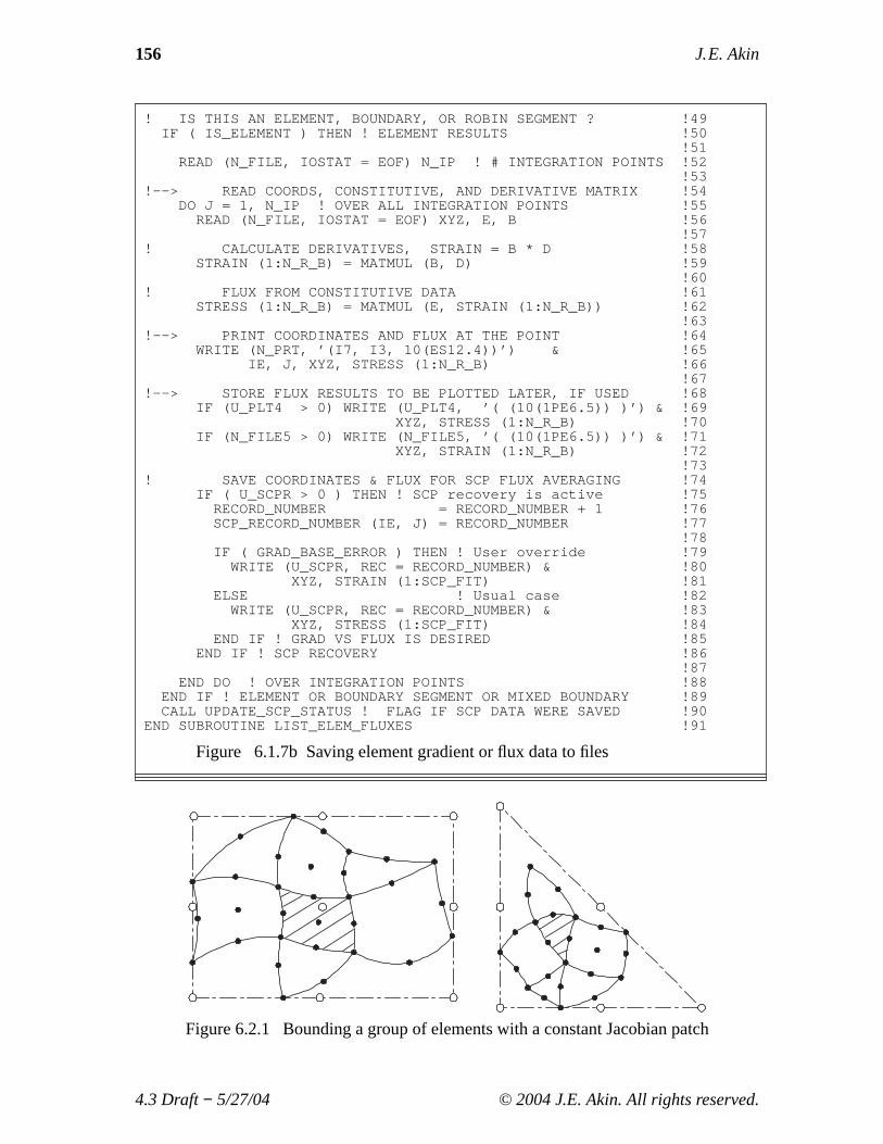
Figure 6.1.7b Saving element gradient or flux data to files

Figure 6.2.1 Bounding a group of elements with a constant Jacobian patch



c. Read the number of quadrature points in the element from U_FLUX;d. Quadrature Point Loop

For each integration point, in routineLIST_ELEM_FLUXES, sequentiallyrecover theXYZ , E, andB arrays from U_FLUX. MultiplyB by the elementdof to get the gradients or strains at the point, and then multiply those by theconstitutive array,E, to get the fluxes, or stresses at the point. The element andquadrature point numbers are then printed along with their coordinates andflux, or stress, components. Lastly, the SCP database is updated byincrementing the record number by one, and then writing the coordinates andflux component arrays to the random access file, U_SCPR, as that record is tobe later randomly recovered in the patch smoothing process. The above detailsare shown in Fig. 6.1.7.

6.2 SCP Nodal Flux Averaging

Having developed the above database on unit U_SCPR we can now average theflux components at every node in each patch and then average them for each node in themesh. Here we assume an element based patch system for calculating the averages. InsubroutineCALC_SCP_AVE_NODE_FLUXES we loop over every element and carryout the least squares fit in its associated patch. Looking ahead to that process we mustselect a polynomial,P, to be used in the patch. We must make a choice for that function.We might select a complete polynomial of a given degree, or a Serendipity polynomial ofa giv en edge degree, etc. In the current implementation the default is to select thatpolynomial to be exactly the same as the polynomial used to interpolate the element forwhich the patch is being constructed. This means that we will select a constant Jacobianpatch "element" that has its local axes parallel to the global axes and completelysurrounds the standard elements that make up the patch. This is easily done by searchingfor the maximum and minimum components of all of the element nodes in the patch.Such a process is illustrated in Fig. 6.2.1 where the active element used to select the patchelement type is shown crosshatched. It would also be easy to allow the user to select apatch type and degree through a keyword control input. The full details of the process aregiven in the source code of Fig.6.2.2 and the main points are outline below.

The least squares flux averaging process is:a. Zero the nodal flux array and the counter for each node.b. Loop over each element in the mesh:

1. Extract its element neighbors to define the patch2. Find the spatial "box" that bounds the patch3. Find the number of quadrature points in the patch (i.e. sum the count in each

element of the patch).4. Determine the element type and thus the patch "element" shape (line, triangle,

hexahedron, etc.) and the corresponding patch polynomial degree.5. Allocate storage for the least squares fit arrays.6. Set the fit matrix row number to zero.


158 J. E. Akin

SUBROUTINE CALC_SCP_AVE_NODE_FLUXES (NODES, X ,L_NEIGH, & ! 0SCP_AVERAGES) ! 1

! * * * * * * * * * * * * * * * * * * * * * * * * * * * * ! 2! CALCULATE THE SUPER_CONVERGENCE_PATCH AVERAGE FLUXES ! 3! AT ALL NODES IN THE MESH VIA THE SVD METHOD ! 4! * * * * * * * * * * * * * * * * * * * * * * * * * * * * ! 5

Use System_Constants ! MAX_NP, NEIGH_P, N_ELEMS, N_PATCH, ! 6! N_QP, SCP_FIT, U_SCPR, ON_BOUNDARY ! 7

Use Elem_Type_Data ! for LAST_LT, LT_* ! 8Use SCP_Type_Data ! for SCP_H (SCP_N), SCP_DLH ! 9

IMPLICIT NONE ! 10INTEGER, INTENT (IN) :: NODES (L_S_TOT, NOD_PER_EL) ! 11INTEGER, INTENT (IN) :: L_NEIGH (NEIGH_P, N_PATCH) ! 12REAL(DP), INTENT (IN) :: X (MAX_NP, N_SPACE) ! 13REAL(DP), INTENT (OUT) :: SCP_AVERAGES (MAX_NP, SCP_FIT) ! 14

! 15INTEGER :: MEMBERS (NEIGH_P+1) ! ELEMENTS IN PATCH ! 16INTEGER :: SCP_COUNTS (MAX_NP) ! PATCH HITS PER NODE ! 17INTEGER :: POINTS ! CURRENT PATCH EQ SIZE ! 18INTEGER :: L_IN_PATCH ! NUM OF ELEMS IN PATCH ! 19INTEGER :: FIT, IL, IP, IQ, LM ! LOOPS ! 20INTEGER :: ROW ! IN PATCH ARRAYS ! 21INTEGER :: LT, REC_LM_IQ, SCP_STAT ! MEMBER OF PATCH ! 22INTEGER, PARAMETER :: ONE = 1 ! 23

! 24REAL(DP) :: XYZ_MIN (N_SPACE), XYZ_MAX (N_SPACE) ! BOUNDS ! 25REAL(DP) :: XYZ (N_SPACE), FLUX (N_R_B) ! PT, FLUX ! 26REAL(DP) :: POINT (N_SPACE) ! SCP POINT ! 27

! 28REAL(DP), ALLOCATABLE :: PATCH_SQ (:, :) ! SCRATCH ARRAY ! 29REAL(DP), ALLOCATABLE :: PATCH_DAT (:, :) ! SCRATCH ARRAY ! 30REAL(DP), ALLOCATABLE :: PATCH_P (:, :) ! SCRATCH ARRAY ! 31REAL(DP), ALLOCATABLE :: PATCH_WRK (:) ! SCRATCH ARRAY ! 32REAL(DP), ALLOCATABLE :: PATCH_FIT (:, :) ! ANSWERS ! 33

! 34! L_S_TOT = TOTAL NUMBER OF ELEMENTS & THEIR SEGMENTS ! 35! L_NEIGH = ELEMENTS FORMING THE PATCH ! 36! L_TYPE = ELEMENT TYPE NUMBER ! 37! LT = ELEMENT TYPE NUMBER (IF USED) ! 38! LT_QP = NUMBER OF QUADRATURE PTS FOR ELEMENT TYPE ! 39! MAX_NP = NUMBER OF SYSTEM NODES ! 40! MEMBERS = ELEMENT NUMBERS MACKING UP A SCP ! 41! NEIGH_P = MAXIMUM NUMBER OF ELEMENTS IN A PATCH ! 42! NOD_PER_EL = NUMBER OF NODES PER ELEMENT ! 43! NODES = NODAL INCIDENCES OF ALL ELEMENTS ! 44! N_ELEMS = NUMBER OF ELEMENTS IN SYSTEM ! 45! N_PATCH = NUMBER OF PATCHES, MAX_NP OR N_ELEMS ! 46! N_QP = MAXIMUN NUMBER OF QUADRATURE POINTS, >= LT_QP ! 47! N_R_B = NUMBER OF ROWS IN B AND E MATRICES ! 48! N_SPACE = DIMENSION OF SPACE ! 49! PATCH_FIT = LOCAL PATCH VALUES FOR FLUX AT ITS NODES ! 50! POINT = LOCAL POINT IN PATCH INTERPOLATION SPACE ! 51! POINTS = TOTAL NUMBER OF QUADRATURE POINTS IN PATCH ! 52! SCP_AVERAGES = AVERAGED FLUXES AT ALL NODES IN MESH ! 53! SCP_FIT = NUMBER IF TERMS BEING FIT, OR AVERAGED ! 54! SCP_H = INTERPOLATION FUNCTIONS OF PATCH, USUALLY H ! 55

Figure 6.2.2a Interface and data for flux averages



! SCP_N = NUMBER OF NODES PER PATCH ! 56! SCP_RECORD_NUMBER = SCP DIRECT ACCESS RECORD LOCATOR ! 57! U_SCPR = SUPER_CONVERGENT PATCH RECOVERY UNIT ! 58! X = COORDINATES OF SYSTEM NODES ! 59! XYZ = SPACE COORDINATES AT A POINT ! 60! XYZ_MAX = UPPER BOUNDS FOR SCP GEOMETRY ! 61! XYZ_MIN = LOWER BOUNDS FOR SCP GEOMETRY ! 62

! 63LT=1 ; LAST_LT=0 ; SCP_COUNTS=0 ; SCP_AVERAGES=0 ! 64

! 65IF ( N_PATCH == 0 ) THEN ! No data supplied ! 66

PRINT *,’NO PATCHS GIVEN, SKIPPING AVERAGES’; RETURN ! 67END IF ! 68

! 69DO IP = 1, N_PATCH ! LOOP OVER EACH PATCH ! 70

MEMBERS = 0 ; POINTS = 0 ! INITIALIZE ! 71! 72

! ELEMENT OR NODAL CENTERED PATCH TYPE ! 73IF ( .NOT. SCP_NEIGH_PT ) THEN ! ELEMENT BASED ! 74

! GET ELEMENT NEIGHBORS TO DEFINE THE PATCH ! 75MEMBERS = (/ IP, L_NEIGH (:, IP) /) ! 76

ELSE ! NODAL BASED PATCH OF ELEMENTS ! 77! GET ELEMENT NEIGHBORS TO DEFINE THE PATCH ! 78

MEMBERS = L_NEIGH (:, IP) ! 79END IF ! PATCH BASIS ! 80

! 81L_IN_PATCH = COUNT ( MEMBERS > 0 ) ! 82IF ( L_IN_PATCH <= 1 ) CYCLE ! TO AN ACTIVE PATCH ! 83

! 84! FIND TYPE OF SCP NEEDED HERE, VERIFY GEOMETRY ! 85

CALL DETERMINE_SCP_BOUNDS (L_IN_PATCH, MEMBERS, & ! 86NODES, X, XYZ_MIN, XYZ_MAX, POINTS) ! 87

! 88IF ( PATCH_ALLOC_STATUS ) THEN ! DEALLOCATE ARRAYS ! 89

DEALLOCATE (PATCH_WRK) ; DEALLOCATE (PATCH_SQ ) ! 90DEALLOCATE (PATCH_FIT) ; DEALLOCATE (PATCH_DAT) ! 91DEALLOCATE (PATCH_P ) ; PATCH_ALLOC_STATUS=.FALSE. ! 92

END IF ! STATUS CHECK ! 93! 94

! ALLOCATE NEXT SET OF LOCAL PATCH RELATED ARRAYS ! 95ALLOCATE ( PATCH_P (POINTS, SCP_N ) ) ! 96ALLOCATE ( PATCH_DAT (POINTS, SCP_FIT) ) ! 97ALLOCATE ( PATCH_FIT (SCP_N , N_R_B ) ) ! 98ALLOCATE ( PATCH_SQ (SCP_N , SCP_N ) ) ! 99ALLOCATE ( PATCH_WRK (SCP_N ) ) !100PATCH_ALLOC_STATUS = .TRUE. !101

!102! ZERO PATCH WORKSPACE AND RESULTS ARRYS !103

PATCH_P = 0.d0 ; PATCH_DAT = 0.d0 ; PATCH_FIT = 0.d0 !104PATCH_SQ = 0.d0 ; PATCH_WRK = 0.d0 !105

!106

Figure 6.2.2b Establish bounds and dynamic memory for each patch


160 J. E. Akin

! PREPARE LEAST SQUARES FIT MATRICES !107LAST_LT = 0 ; ROW = 0 ! INITIALIZE !108DO IL = 1, L_IN_PATCH ! PATCH MEMBER LOOP !109

LM = MEMBERS (IL) ! ELEMENT IN PATCH !110!111

! GET ELEMENT TYPE NUMBER !112IF (N_L_TYPE > 1) LT=L_TYPE (LM) !113IF ( LT /= LAST_LT ) THEN ! ELEMENT TYPE !114

CALL GET_ELEM_TYPE_DATA (LT) ! TYPE CONTROLS !115LAST_LT = LT !116

END IF ! a new element type and scp type !117!118

DO IQ = 1, LT_QP ! LOOP OVER GAUSS POINTS !119ROW = ROW + 1 ! UPDATE LOCATION !120

!121! RECOVER EACH FLUX VECTOR TO FOR LEAST SQ FIX !122

REC_LM_IQ = SCP_RECORD_NUMBER (LM, IQ) ! REC NUMBER !123!124

! GET GAUSS PT COORD & FLUX SAVED IN LIST_ELEM_FLUXES !125READ (U_SCPR,REC=REC_LM_IQ,IOSTAT=SCP_STAT) XYZ, FLUX !126SELECT CASE ( SCP_STAT ) ! for read status !127

CASE (:-1) !128STOP ’EOR OR EOF, CALC_SCP_AVE_NODE_FLUXES’ !129

CASE (1:) !130PRINT *,’MEMBER ELEMENT = ’, LM, ’ AT POINT ’, IQ !131PRINT *,’REC_LM_IQ = ’, REC_LM_IQ !132STOP ’BAD SCP_STAT, CALC_SCP_AVE_NODE_FLUXES’ !133

CASE DEFAULT ! NO READ ERROR !134END SELECT ! RANDOM ACCESS READ ERROR !135

!136! CONVERT IQ XYZ TO LOCAL PATCH POINT !137

POINT = GET_SCP_PT_AT_XYZ (XYZ, XYZ_MIN, XYZ_MAX) !138!139

! EVALUATE PATCH INTERPOLATION AT LOCAL POINT !140IF ( .NOT. SCP_SCAL_ALLOC ) CALL & !141

ALLOCATE_SCP_INTERPOLATIONS !142CALL GEN_ELEM_SHAPE (POINT,SCP_H,SCP_N,N_SPACE,ONE) !143

!144! INSERT FLUX & INTERPOLATIONS INTO PATCH MATRICES !145

PATCH_DAT (ROW, 1:N_R_B) = FLUX (:) !146PATCH_P (ROW, :) = SCP_H (:) !147

END DO ! FOR EACH IQ FLUX VECTOR !148!149

END DO ! FOR EACH IL PATCH MEMBER !150! ASSEMBLY OF PATCH COMPLETED !151

!152! VALIDATE CURRENT PATCH !153

IF ( POINTS < SCP_N ) THEN !154PRINT *,’WARNING: SKIPPING PATCH ’, & !155

IP, ’ WITH ONLY ’, POINTS, ’ EQUATIONS’ !156CYCLE ! TO NEXT PATCH !157

END IF ! INSUFFICIENT DATA !158

Figure 6.2.2c Build the least squares fit in each patch



! USE SINGULAR VALUE DECOMPOSITION SOLUTION METHOD !159CALL SVDC_FACTOR (PATCH_P,POINTS,SCP_N,PATCH_WRK,PATCH_SQ) !160WHERE ( PATCH_WRK < EPSILON(1.d0) ) PATCH_WRK = 0.D0 !161

!162DO FIT = 1, N_R_B ! LOOP FOR EACH FLUX COMPONENT !163

CALL SVDC_BACK_SUBST (PATCH_P, PATCH_WRK, PATCH_SQ, & !164POINTS, SCP_N, PATCH_DAT (:, FIT),& !165PATCH_FIT (:, FIT)) !166

END DO ! FOR FLUXES COMPONENTS !167!168

! INTERPOLATE AVERAGES TO ALL NODES IN THE PATCH. SCATTER !169! PATCH NODAL AVERAGES TO SYSTEM NODES, INCREMENT COUNTS !170

!171IF (DEBUG_SCP .AND. IP==1) PRINT *,’AVERAGING FLUXES’ !172CALL EVAL_SCP_FIT_AT_PATCH_NODES (IP, NODES, X, & !173

L_IN_PATCH,MEMBERS, XYZ_MIN, XYZ_MAX, PATCH_FIT, & !174SCP_AVERAGES, SCP_COUNTS) !175

!176! NOTE: use Loubignac iteration here for new solution !177

!178! DEALLOCATE LOCAL PATCH RELATED ARRAYS !179

IF (SCP_SCAL_ALLOC) CALL DEALLOCATE_SCP_INTERPOLATIONS !180DEALLOCATE (PATCH_WRK) ; DEALLOCATE (PATCH_SQ ) !181DEALLOCATE (PATCH_FIT) ; DEALLOCATE (PATCH_DAT) !182DEALLOCATE (PATCH_P ) ; PATCH_ALLOC_STATUS=.FALSE. !183

!184END DO ! FOR EACH IP PATCH IN MESH !185

!186! FINALLY, AVERAGE FLUXES FOR EACH NODAL HIT COUNT !187

DO FIT = 1, MAX_NP ! FOR ALL NODES !188IF ( SCP_COUNTS (FIT) /= 0 ) THEN ! ACTIVE NODE !189

SCP_AVERAGES (FIT, :) = SCP_AVERAGES (FIT, :) & !190/ SCP_COUNTS (FIT) !191

ELSE ! could skip since initialized !192SCP_AVERAGES (FIT, :) = 0.D0 !193

END IF !194END DO ! FOR (AN UNWEIGHTED) AVERAGE !195

!196! REPORT AVERAGED MAX & MIN VALUES AND LOCATIONS !197

CALL MAX_AND_MIN_SCP_AVE_F90 (SCP_AVERAGES) !198END SUBROUTINE CALC_SCP_AVE_NODE_FLUXES !199

Figure 6.2.2d Factor each patch then average at all nodes

7. For each element in the patch loop over the following steps:A. Find its type and quadrature ruleB. Loop over each of its quadrature points

1) Increment the row number by one.2) Use the element number and quadrature point number pair as

subscripts in theSCP_RECORD_NUMBER function to recover therandom record number for that point.

3) Read the physical coordinates and flux components from randomaccess file U_SCPR by using that record number.

4) Use the constant Jacobian of the patch to convert the physicallocation to the corresponding non-dimensional coordinates in thepatch. Note that this helps reduce the numerical ill-conditioning that


162 J. E. Akin

is common in a least squares fit process.5) Evaluate the patch interpolation polynomial at the local point (by

utilizing the standard element interpolation library). Insert it into theleft hand side of this row of the coefficient matrix.

6) Substitute the flux components into the right hand side data matrix, inthe same row. Of course the number of columns on the right handside is the same as the number of flux components. This is also thesize of the patch result matrix,a, to be computed.

8. Having completed the loop over all the elements in this patch we now hav e therectangular arrays cited in Eq. 12.28 but we have not computed their actualmatrix products as shown in Eq. 12.29. While that equation is the standardway to describe a least squares fit we do not actually use that process. Instead,we try to avoid possible numerical ill-conditioning by using an equivalent butmore powerful process called the singular value decomposition algorithm [10].That process first factors the associated patch square matrix (in subroutineSVDC_FACTOR) and then recovers the rectangular array of local continuouspatch nodal flux values (with subroutineSVDC_BACK_SUBST). However,we want smooth flux values at the actual modes of the elements, not values atthe patch nodes. Thus, for the elements in question we need to interpolate thepatch results back to the system nodes contained within the current patch.

9) Loop over nodes in this patch:a) Use the constant patch Jacobian to convert the node coordinates to non-

dimensional coordinates of the patchb) Evaluate the patch interpolation matrix,SCP_HSCP_H , at each node point. It is

usually the same as the core element interpolation functionsH.c) Compute the flux components at the node by the matrix product of

SCP_HSCP_H and the continuous gradients at the patch nodes,a.d) Increment the nodal counter for patch contributions by one and scatter the

node flux components to the rectangular system flux nodal array.C. Optional Improvement of the Solution

At this stage in the SCP process one can use the least square smoothed gradients inthis patch to get a locally improved solution value estimate at all of the patch’sinterior nodes. However, one may want to just do so for the single parent elementabout which the patch was constructed. The algorithm is a form of the Loubignac[9] iterative process:

1) Read or reform element matrices,Se andCe, here;2) Use a higher order quadrature rule to form the equilibrating vector

Ve =Ωe∫ B* (σσ * − σσ ) dΩ ;

3) Assemble the elements in the patch into a local linear system:

S* φφnew = C − V ;

4) Apply the previous solution as essential boundary conditions at all nodes on thepatch boundary;



5) Solve for the new interior node values (always a small system but especiallysmall for a patch of elements around a single node as in original ZZ patchpaper). Call themφφ *

e .6) Compute norm ofφφ e − φφ *

e to use as an additional term in the final errorestimator.

d. Final nodal flux average.

As shown in Fig. 6.2.3, most nodes are associated with more than one patch.Having processed every patch for the mesh each node has now received as manynodal flux estimates as there were patches that contained that node. We finalize thenodal flux values by simply dividing each node’s flux components sums by thatinteger counter, print the result, and re-save them in the rectangular arraySCP_AVERAGES for use by the element error estimator or other user-defined post-processing.

6.3 Computing the SCP Element Error Estimates

For a homogeneous domain, or sub-domain, the above nodal averaging processprovides a continuous flux approximation that should be much closer to the true solutionthan the element discontinuous fluxes. Thus, it is reasonable to base the element errorestimator on the average nodal fluxes from the SCP process. Basically, we will want tointegrate the difference between the spatial distributions of the two flux estimates so thatwe can calculate the error norms of interest in each element. Then we will sum thosescalar values over all elements so that we can establish the relative errors and how theycompare to the allowed value specified by the user. Of course, we will evaluate theelement norms by numerical integration. This will require a higher order quadrature rule

Figure 6.2.3 Overlapping patches give multiple node estimates


164 J. E. Akin

than the one needed to evaluate the element square matrix because the interpolationfunction,P (which is usuallyH), is of higher polynomial degree than theB matrix (whichcontains the derivatives ofH) used in forming the element square matrix.

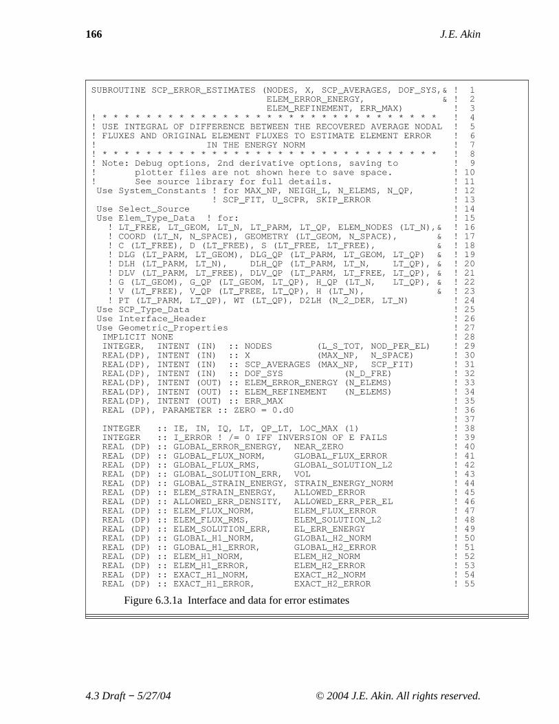
SubroutineSCP_ERROR_ESTIMATESimplements the major steps outlined below.1. Preliminary Setupa. Initialize all of the norms to zero.b. If the mesh has a constant constitutive matrix,E, then recover it and invert it once

for later use in calculating the energy norm.2. Loop over all elements in the mesh:a. Recover the element type (shape, number of nodes, quadrature rule forB, etc.)b. Determine the quadrature rule to integrate theP array (here theH array), allocate

storage for that array to be pre-computed at each quadrature point, and then fillthose arrays.

c. Extract the element’s node numbers, coordinates, anddof.d. At each node on the element gather the continuous nodal flux components from the

system SCP averages,ae ⊂ a .e. Numerical integration loop over the element to form element norms and increment

system norms:1. Recover theH array at the point and its local derivatives.2. Obtain the physical coordinates, Jacobian and its inverse.3. If the L2 norm of the solution is desired, interpolate for the value at the point.

Increment theL2 norm integral. If the exact solution has been provided, thencompute its norm also.

4. Compute the physical gradients of the original finite element solution. Form theBmatrix at the point for the current application, ˆεε = B φφ . If the constitutive array,E,is smoothly varying, then we could evaluate it at this point (and compute itsinverse). Otherwise, we employ theE matrix saved in the preliminary setup. Nowwe recover the standard element flux estimate by matrix multiplication, ˆσσ = E εε .We can also increment theL2 norm of this term if desired.

5. Now we are ready to recover the continuous flux values and approximate the stresserror. We simply carry out the matrix product of the interpolation functions,H, andthe nodal fluxes,a, at the quadrature point.

σσ * = H a

The difference between these components and those from the previous step areformed to define the stress error

eσ = σσ * − σσ .

If desired the square of this term (its dot product with itself) is obtained for itsincrement to theL2 stress norm.

6. In this implementation we almost always use the flux error to compute the errorenergy norm, so at this stage we form the related triple matrix product,eT

σ E−1eσ ,and increment the quadrature point contribution to the element norm



||ee||2 =nq

qΣ(σσ * − σσ )T

q E−1q (σσ * − σσ )q .

If the user has supplied an expression for the exact flux components, then they areevaluated at the physical coordinates, and the correspondingL2 and error energy normsare updated for later comparisons and to find the effectivity index.

Having incremented all of the element norms, they are complete at the end of thisquadrature loop for the current element. The active element norm values are then addedto the current values of the corresponding system norms. At times we also want to usethe element and system volume measures so that we can get some norm volumetricav erages. Thus, the determinant of the Jacobian at the above points are also used toobtain the element volumes so that they are available for these optional calculations.

Upon completing the loop over all elements we have the element norms, the elementvolume, the system norms,

||e||2 =ne

eΣ ||ee||2 ,

and the system volume. At this point we can then carry out the element adaptivityprocesses outlined at the end of the previous chapter. The coding details associated withthese steps are in the single subroutine but are broken out into major segments inFig. 6.3.1.

6.4 Hessian Matrix *

There are times when one is also interested in the estimates of the second derivativesof the solution with respect to the spatial coordinates. Examples include the applicationof the Streamline Upwind Petrov Galerkin (SUPG) method for advection-diffusionproblems [6] and the inclusion of "stabilization" (or governing PDE residual) terms inthe solution of the Navier-Stokes equations. The matrix of second-order partialderivatives of a function is called the Hessian matrix. If the function isC2, (that is, hascontinuous second derivatives) the Hessian is symmetric due to the equality of the mixedpartial derivatives. If one is employing high-order interpolation elements, one couldproceed with direct estimates of the second derivatives at the element level. Of course,we would expect a decrease in accuracy compared to the element gradient estimates.Even with higher order elements the first and second derivatives are not continuous at theboundaries of surrounding elements (that is, elements that would make up a patch).Thus, a Hessian matrix based on a patch calculation will usually not be symmetric.Assuming the use of parametric elements, we need to employ the Jacobian. The Jacobiandefines the mapping from the parametric space the physical space. In two dimensions :


166 J. E. Akin

SUBROUTINE SCP_ERROR_ESTIMATES (NODES, X, SCP_AVERAGES, DOF_SYS,& ! 1ELEM_ERROR_ENERGY, & ! 2ELEM_REFINEMENT, ERR_MAX) ! 3

! * * * * * * * * * * * * * * * * * * * * * * * * * * * * * * * ! 4! USE INTEGRAL OF DIFFERENCE BETWEEN THE RECOVERED AVERAGE NODAL ! 5! FLUXES AND ORIGINAL ELEMENT FLUXES TO ESTIMATE ELEMENT ERROR ! 6! IN THE ENERGY NORM ! 7! * * * * * * * * * * * * * * * * * * * * * * * * * * * * * * * ! 8! Note: Debug options, 2nd derivative options, saving to ! 9! plotter files are not shown here to save space. ! 10! See source library for full details. ! 11

Use System_Constants ! for MAX_NP, NEIGH_L, N_ELEMS, N_QP, ! 12! SCP_FIT, U_SCPR, SKIP_ERROR ! 13

Use Select_Source ! 14Use Elem_Type_Data ! for: ! 15

! LT_FREE, LT_GEOM, LT_N, LT_PARM, LT_QP, ELEM_NODES (LT_N),& ! 16! COORD (LT_N, N_SPACE), GEOMETRY (LT_GEOM, N_SPACE), & ! 17! C (LT_FREE), D (LT_FREE), S (LT_FREE, LT_FREE), & ! 18! DLG (LT_PARM, LT_GEOM), DLG_QP (LT_PARM, LT_GEOM, LT_QP) & ! 19! DLH (LT_PARM, LT_N), DLH_QP (LT_PARM, LT_N, LT_QP), & ! 20! DLV (LT_PARM, LT_FREE), DLV_QP (LT_PARM, LT_FREE, LT_QP), & ! 21! G (LT_GEOM), G_QP (LT_GEOM, LT_QP), H_QP (LT_N, LT_QP), & ! 22! V (LT_FREE), V_QP (LT_FREE, LT_QP), H (LT_N), & ! 23! PT (LT_PARM, LT_QP), WT (LT_QP), D2LH (N_2_DER, LT_N) ! 24

Use SCP_Type_Data ! 25Use Interface_Header ! 26Use Geometric_Properties ! 27

IMPLICIT NONE ! 28INTEGER, INTENT (IN) :: NODES (L_S_TOT, NOD_PER_EL) ! 29REAL(DP), INTENT (IN) :: X (MAX_NP, N_SPACE) ! 30REAL(DP), INTENT (IN) :: SCP_AVERAGES (MAX_NP, SCP_FIT) ! 31REAL(DP), INTENT (IN) :: DOF_SYS (N_D_FRE) ! 32REAL(DP), INTENT (OUT) :: ELEM_ERROR_ENERGY (N_ELEMS) ! 33REAL(DP), INTENT (OUT) :: ELEM_REFINEMENT (N_ELEMS) ! 34REAL(DP), INTENT (OUT) :: ERR_MAX ! 35REAL (DP), PARAMETER :: ZERO = 0.d0 ! 36

! 37INTEGER :: IE, IN, IQ, LT, QP_LT, LOC_MAX (1) ! 38INTEGER :: I_ERROR ! /= 0 IFF INVERSION OF E FAILS ! 39REAL (DP) :: GLOBAL_ERROR_ENERGY, NEAR_ZERO ! 40REAL (DP) :: GLOBAL_FLUX_NORM, GLOBAL_FLUX_ERROR ! 41REAL (DP) :: GLOBAL_FLUX_RMS, GLOBAL_SOLUTION_L2 ! 42REAL (DP) :: GLOBAL_SOLUTION_ERR, VOL ! 43REAL (DP) :: GLOBAL_STRAIN_ENERGY, STRAIN_ENERGY_NORM ! 44REAL (DP) :: ELEM_STRAIN_ENERGY, ALLOWED_ERROR ! 45REAL (DP) :: ALLOWED_ERR_DENSITY, ALLOWED_ERR_PER_EL ! 46REAL (DP) :: ELEM_FLUX_NORM, ELEM_FLUX_ERROR ! 47REAL (DP) :: ELEM_FLUX_RMS, ELEM_SOLUTION_L2 ! 48REAL (DP) :: ELEM_SOLUTION_ERR, EL_ERR_ENERGY ! 49REAL (DP) :: GLOBAL_H1_NORM, GLOBAL_H2_NORM ! 50REAL (DP) :: GLOBAL_H1_ERROR, GLOBAL_H2_ERROR ! 51REAL (DP) :: ELEM_H1_NORM, ELEM_H2_NORM ! 52REAL (DP) :: ELEM_H1_ERROR, ELEM_H2_ERROR ! 53REAL (DP) :: EXACT_H1_NORM, EXACT_H2_NORM ! 54REAL (DP) :: EXACT_H1_ERROR, EXACT_H2_ERROR ! 55

Figure 6.3.1a Interface and data for error estimates



REAL (DP) :: EXACT_SOL_L2, EX_ERR_ENERGY ! 56REAL (DP) :: EXACT_FLUX_ERROR, EXACT_FLUX_NORM ! 57REAL (DP) :: EXACT_STRAIN_ENERGY, EXACT_ERR_ENERGY ! 58REAL (DP) :: DET, DET_WT, TEMP, TEST, SCP_VOLUME ! 59REAL (DP), ALLOCATABLE :: DOF_EL (:, :) ! D RESHAPE ! 60

! 61! Automatic Arrays ! 62

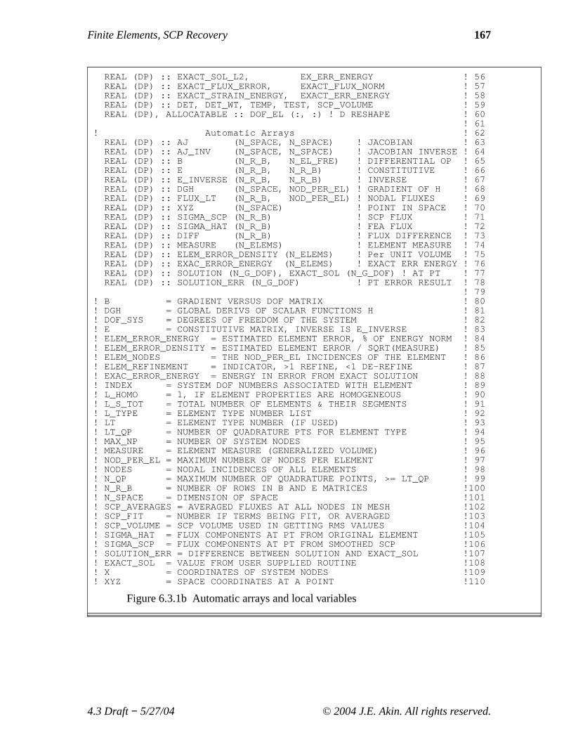
REAL (DP) :: AJ (N_SPACE, N_SPACE) ! JACOBIAN ! 63REAL (DP) :: AJ_INV (N_SPACE, N_SPACE) ! JACOBIAN INVERSE ! 64REAL (DP) :: B (N_R_B, N_EL_FRE) ! DIFFERENTIAL OP ! 65REAL (DP) :: E (N_R_B, N_R_B) ! CONSTITUTIVE ! 66REAL (DP) :: E_INVERSE (N_R_B, N_R_B) ! INVERSE ! 67REAL (DP) :: DGH (N_SPACE, NOD_PER_EL) ! GRADIENT OF H ! 68REAL (DP) :: FLUX_LT (N_R_B, NOD_PER_EL) ! NODAL FLUXES ! 69REAL (DP) :: XYZ (N_SPACE) ! POINT IN SPACE ! 70REAL (DP) :: SIGMA_SCP (N_R_B) ! SCP FLUX ! 71REAL (DP) :: SIGMA_HAT (N_R_B) ! FEA FLUX ! 72REAL (DP) :: DIFF (N_R_B) ! FLUX DIFFERENCE ! 73REAL (DP) :: MEASURE (N_ELEMS) ! ELEMENT MEASURE ! 74REAL (DP) :: ELEM_ERROR_DENSITY (N_ELEMS) ! Per UNIT VOLUME ! 75REAL (DP) :: EXAC_ERROR_ENERGY (N_ELEMS) ! EXACT ERR ENERGY ! 76REAL (DP) :: SOLUTION (N_G_DOF), EXACT_SOL (N_G_DOF) ! AT PT ! 77REAL (DP) :: SOLUTION_ERR (N_G_DOF) ! PT ERROR RESULT ! 78

! 79! B = GRADIENT VERSUS DOF MATRIX ! 80! DGH = GLOBAL DERIVS OF SCALAR FUNCTIONS H ! 81! DOF_SYS = DEGREES OF FREEDOM OF THE SYSTEM ! 82! E = CONSTITUTIVE MATRIX, INVERSE IS E_INVERSE ! 83! ELEM_ERROR_ENERGY = ESTIMATED ELEMENT ERROR, % OF ENERGY NORM ! 84! ELEM_ERROR_DENSITY = ESTIMATED ELEMENT ERROR / SQRT(MEASURE) ! 85! ELEM_NODES = THE NOD_PER_EL INCIDENCES OF THE ELEMENT ! 86! ELEM_REFINEMENT = INDICATOR, >1 REFINE, <1 DE-REFINE ! 87! EXAC_ERROR_ENERGY = ENERGY IN ERROR FROM EXACT SOLUTION ! 88! INDEX = SYSTEM DOF NUMBERS ASSOCIATED WITH ELEMENT ! 89! L_HOMO = 1, IF ELEMENT PROPERTIES ARE HOMOGENEOUS ! 90! L_S_TOT = TOTAL NUMBER OF ELEMENTS & THEIR SEGMENTS ! 91! L_TYPE = ELEMENT TYPE NUMBER LIST ! 92! LT = ELEMENT TYPE NUMBER (IF USED) ! 93! LT_QP = NUMBER OF QUADRATURE PTS FOR ELEMENT TYPE ! 94! MAX_NP = NUMBER OF SYSTEM NODES ! 95! MEASURE = ELEMENT MEASURE (GENERALIZED VOLUME) ! 96! NOD_PER_EL = MAXIMUM NUMBER OF NODES PER ELEMENT ! 97! NODES = NODAL INCIDENCES OF ALL ELEMENTS ! 98! N_QP = MAXIMUM NUMBER OF QUADRATURE POINTS, >= LT_QP ! 99! N_R_B = NUMBER OF ROWS IN B AND E MATRICES !100! N_SPACE = DIMENSION OF SPACE !101! SCP_AVERAGES = AVERAGED FLUXES AT ALL NODES IN MESH !102! SCP_FIT = NUMBER IF TERMS BEING FIT, OR AVERAGED !103! SCP_VOLUME = SCP VOLUME USED IN GETTING RMS VALUES !104! SIGMA_HAT = FLUX COMPONENTS AT PT FROM ORIGINAL ELEMENT !105! SIGMA_SCP = FLUX COMPONENTS AT PT FROM SMOOTHED SCP !106! SOLUTION_ERR = DIFFERENCE BETWEEN SOLUTION AND EXACT_SOL !107! EXACT_SOL = VALUE FROM USER SUPPLIED ROUTINE !108! X = COORDINATES OF SYSTEM NODES !109! XYZ = SPACE COORDINATES AT A POINT !110

Figure 6.3.1b Automatic arrays and local variables


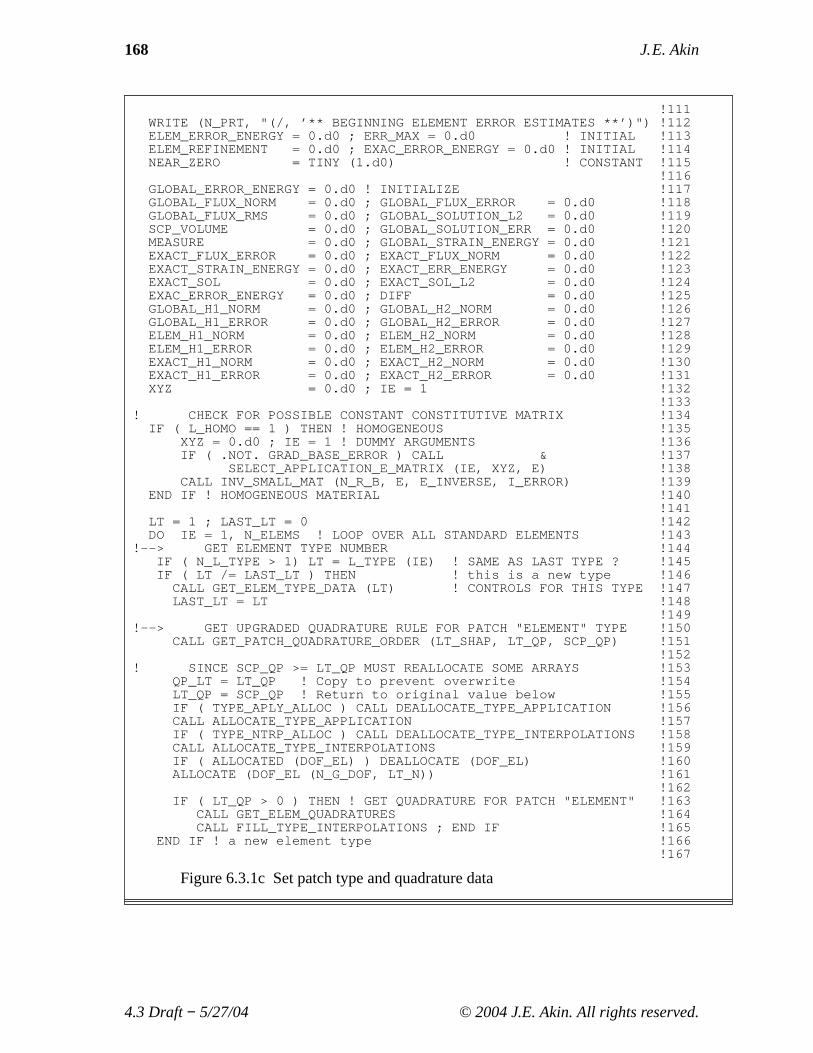
168 J. E. Akin

!111WRITE (N_PRT, "(/, ’** BEGINNING ELEMENT ERROR ESTIMATES **’)") !112ELEM_ERROR_ENERGY = 0.d0 ; ERR_MAX = 0.d0 ! INITIAL !113ELEM_REFINEMENT = 0.d0 ; EXAC_ERROR_ENERGY = 0.d0 ! INITIAL !114NEAR_ZERO = TINY (1.d0) ! CONSTANT !115

!116GLOBAL_ERROR_ENERGY = 0.d0 ! INITIALIZE !117GLOBAL_FLUX_NORM = 0.d0 ; GLOBAL_FLUX_ERROR = 0.d0 !118GLOBAL_FLUX_RMS = 0.d0 ; GLOBAL_SOLUTION_L2 = 0.d0 !119SCP_VOLUME = 0.d0 ; GLOBAL_SOLUTION_ERR = 0.d0 !120MEASURE = 0.d0 ; GLOBAL_STRAIN_ENERGY = 0.d0 !121EXACT_FLUX_ERROR = 0.d0 ; EXACT_FLUX_NORM = 0.d0 !122EXACT_STRAIN_ENERGY = 0.d0 ; EXACT_ERR_ENERGY = 0.d0 !123EXACT_SOL = 0.d0 ; EXACT_SOL_L2 = 0.d0 !124EXAC_ERROR_ENERGY = 0.d0 ; DIFF = 0.d0 !125GLOBAL_H1_NORM = 0.d0 ; GLOBAL_H2_NORM = 0.d0 !126GLOBAL_H1_ERROR = 0.d0 ; GLOBAL_H2_ERROR = 0.d0 !127ELEM_H1_NORM = 0.d0 ; ELEM_H2_NORM = 0.d0 !128ELEM_H1_ERROR = 0.d0 ; ELEM_H2_ERROR = 0.d0 !129EXACT_H1_NORM = 0.d0 ; EXACT_H2_NORM = 0.d0 !130EXACT_H1_ERROR = 0.d0 ; EXACT_H2_ERROR = 0.d0 !131XYZ = 0.d0 ; IE = 1 !132

!133! CHECK FOR POSSIBLE CONSTANT CONSTITUTIVE MATRIX !134

IF ( L_HOMO == 1 ) THEN ! HOMOGENEOUS !135XYZ = 0.d0 ; IE = 1 ! DUMMY ARGUMENTS !136IF ( .NOT. GRAD_BASE_ERROR ) CALL & !137

SELECT_APPLICATION_E_MATRIX (IE, XYZ, E) !138CALL INV_SMALL_MAT (N_R_B, E, E_INVERSE, I_ERROR) !139

END IF ! HOMOGENEOUS MATERIAL !140!141

LT = 1 ; LAST_LT = 0 !142DO IE = 1, N_ELEMS ! LOOP OVER ALL STANDARD ELEMENTS !143

!--> GET ELEMENT TYPE NUMBER !144IF ( N_L_TYPE > 1) LT = L_TYPE (IE) ! SAME AS LAST TYPE ? !145IF ( LT /= LAST_LT ) THEN ! this is a new type !146

CALL GET_ELEM_TYPE_DATA (LT) ! CONTROLS FOR THIS TYPE !147LAST_LT = LT !148

!149!--> GET UPGRADED QUADRATURE RULE FOR PATCH "ELEMENT" TYPE !150

CALL GET_PATCH_QUADRATURE_ORDER (LT_SHAP, LT_QP, SCP_QP) !151!152

! SINCE SCP_QP >= LT_QP MUST REALLOCATE SOME ARRAYS !153QP_LT = LT_QP ! Copy to prevent overwrite !154LT_QP = SCP_QP ! Return to original value below !155IF ( TYPE_APLY_ALLOC ) CALL DEALLOCATE_TYPE_APPLICATION !156CALL ALLOCATE_TYPE_APPLICATION !157IF ( TYPE_NTRP_ALLOC ) CALL DEALLOCATE_TYPE_INTERPOLATIONS !158CALL ALLOCATE_TYPE_INTERPOLATIONS !159IF ( ALLOCATED (DOF_EL) ) DEALLOCATE (DOF_EL) !160ALLOCATE (DOF_EL (N_G_DOF, LT_N)) !161

!162IF ( LT_QP > 0 ) THEN ! GET QUADRATURE FOR PATCH "ELEMENT" !163

CALL GET_ELEM_QUADRATURES !164CALL FILL_TYPE_INTERPOLATIONS ; END IF !165

END IF ! a new element type !166!167

Figure 6.3.1c Set patch type and quadrature data



!--> GET ELEMENT NODE NUMBERS, COORD, DOF !168ELEM_NODES = GET_ELEM_NODES (IE, LT_N, NODES) !169CALL ELEM_COORD (LT_N, N_SPACE, X, COORD, ELEM_NODES) !170INDEX = GET_ELEM_INDEX (LT_N, ELEM_NODES) !171D = GET_ELEM_DOF (DOF_SYS) !172DOF_EL = RESHAPE (D, (/ N_G_DOF, LT_N /)) !173

!174!--> EXTRACT SCP NODAL FLUXES (NOW GATHER_LT_SCP_AVERAGES) !175

DO IN = 1, LT_N ! OVER NODES OF ELEMENT !176IF ( ELEM_NODES (IN) < 1 ) CYCLE ! TO VALID NODE !177

FLUX_LT (1:N_R_B, IN) = SCP_AVERAGES ( & !178ELEM_NODES (IN), 1:N_R_B) !179

END DO ! FOR NODES ON ELEMENT !180!181

! INITIALIZE NORMS !182ELEM_FLUX_NORM = 0.d0 ; ELEM_FLUX_ERROR = 0.d0 !183ELEM_FLUX_RMS = 0.d0 ; ELEM_SOLUTION_L2 = 0.d0 !184ELEM_SOLUTION_ERR = 0.d0 ; ELEM_STRAIN_ENERGY = 0.d0 !185EL_ERR_ENERGY = 0.d0 ; EX_ERR_ENERGY = 0.d0 !186VOL = 0.d0 ; ELEM_ERROR_ENERGY (IE) = 0.d0 !187

!188DO IQ = 1, LT_QP ! LOOP OVER QUADRATURE POINTS !189

H = GET_H_AT_QP (IQ) ! INTERPOLATION FUNCTIONS !190XYZ = MATMUL (H, COORD) ! COORDINATES OF PT !191DLH = GET_DLH_AT_QP (IQ) ! LOCAL DERIVATIVES !192

!193! FIND JACOBIAN AT THE PT, INVERSE AND DETERMINANT !194

AJ = MATMUL (DLH (1:N_SPACE, :), COORD) !195CALL INVERT_JACOBIAN (AJ, AJ_INV, DET, N_SPACE) !196IF ( DET <= ZERO ) STOP ’BAD DET, SCP_ERROR_ESTIMATES’ !197DET_WT = DET * WT(IQ) !198

!199IF ( AXISYMMETRIC ) DET_WT = DET_WT * XYZ (1) * TWO_PI !200VOL = VOL + DET_WT ! UPDATE ELEMENT VOLUME !201

!202! EVALUATE SOLUTION L2 NORM (ASSUMING C_0N_G_DOF) !203

SOLUTION = MATMUL (DOF_EL, H) !204ELEM_SOLUTION_L2 = ELEM_SOLUTION_L2 + DET_WT & !205

* DOT_PRODUCT (SOLUTION, SOLUTION) !206!207

! EVALUATE APPLICATION EXACT VALUE & ERROR HERE !208IF ( USE_EXACT ) THEN !209

CALL SELECT_EXACT_SOLUTION (XYZ, EXACT_SOL) !210EXACT_SOL_L2 = EXACT_SOL_L2 + DET_WT & !211

* DOT_PRODUCT (EXACT_SOL, EXACT_SOL) !212SOLUTION_ERR = EXACT_SOL - SOLUTION !213ELEM_SOLUTION_ERR = ELEM_SOLUTION_ERR + DET_WT & !214

* DOT_PRODUCT (SOLUTION_ERR, SOLUTION_ERR) !215END IF ! EXACT SOLUTION GIVEN !216

!217DGH = MATMUL (AJ_INV, DLH) ! GLOBAL DERIVATIVES !218CALL SELECT_APPLICATION_B_MATRIX (DGH, XYZ, B (:,1:LT_FREE)) !219

!220

Figure 6.3.1d Gather continuous flux and integrate error


170 J. E. Akin

! GET LOCAL STRAINS (STORE IN SIGMA_HAT) !221SIGMA_HAT (1:N_R_B) = MATMUL(B(:,1:LT_FREE),D(1:LT_FREE)) !222

!223! APPLY CONSTITUTIVE RELATION (TO STRAINS IN SIGMA_SCP) !224

SIGMA_HAT (1:N_R_B) = MATMUL (E, SIGMA_HAT (1:N_R_B)) !225!226

! GET SCP FLUX ESTIMATES & DIFFERENCE !227SIGMA_SCP (:) = MATMUL (H, TRANSPOSE(FLUX_LT (:,1:LT_N))) !228DIFF = SIGMA_SCP - SIGMA_HAT ! SIGMA ERROR EST !229ELEM_FLUX_NORM = ELEM_FLUX_NORM & !230

+ DET_WT * DOT_PRODUCT (SIGMA_SCP,SIGMA_SCP) !231ELEM_FLUX_ERROR = ELEM_FLUX_ERROR & !232

+ DET_WT * DOT_PRODUCT (DIFF, DIFF) !233!234

! INCREMENT STRAIN ENERGY & ENERGY IN THE ERROR !235TEST = DOT_PRODUCT (SIGMA_SCP,MATMUL(E_INVERSE,SIGMA_SCP)) !236ELEM_STRAIN_ENERGY = ELEM_STRAIN_ENERGY + DET_WT * TEST !237

!238TEST = DOT_PRODUCT (DIFF, MATMUL (E_INVERSE, DIFF)) !239EL_ERR_ENERGY = EL_ERR_ENERGY + DET_WT * TEST !240IF (EL_ERR_ENERGY < NEAR_ZERO ) EL_ERR_ENERGY = 0.d0 !241

!242IF ( USE_EXACT_FLUX ) THEN ! GET EXACT VALUES !243

CALL SELECT_EXACT_FLUX (XYZ, SIGMA_SCP (1:N_R_B)) !244DIFF = SIGMA_SCP - SIGMA_HAT ! EXACT ERROR !245EXACT_FLUX_NORM = EXACT_FLUX_NORM & !246

+ DET_WT * DOT_PRODUCT (SIGMA_SCP, SIGMA_SCP) !247EXACT_FLUX_ERROR = EXACT_FLUX_ERROR & !248

+ DET_WT * DOT_PRODUCT (DIFF, DIFF) !249TEST = DOT_PRODUCT(SIGMA_SCP,MATMUL(E_INVERSE,SIGMA_SCP)) !250EXACT_STRAIN_ENERGY = EXACT_STRAIN_ENERGY + DET_WT*TEST !251TEST = DOT_PRODUCT (DIFF, MATMUL (E_INVERSE, DIFF)) !252EX_ERR_ENERGY = EX_ERR_ENERGY + DET_WT * TEST !253EXACT_ERR_ENERGY = EXACT_ERR_ENERGY + DET_WT * TEST !254

END IF ! EXACT FLUXES GIVEN !255END DO ! OVER ERROR EST QP !256

!257EXAC_ERROR_ENERGY (IE) = EX_ERR_ENERGY + NEAR_ZERO !258ELEM_ERROR_ENERGY (IE) = EL_ERR_ENERGY + NEAR_ZERO !259MEASURE (IE) = VOL !260SCP_VOLUME = SCP_VOLUME + VOL !261

!262! COMBINE AND NORMALIZE ERROR TERMS !263

GLOBAL_STRAIN_ENERGY=GLOBAL_STRAIN_ENERGY+ELEM_STRAIN_ENERGY !264GLOBAL_ERROR_ENERGY = GLOBAL_ERROR_ENERGY + EL_ERR_ENERGY !265GLOBAL_FLUX_NORM = GLOBAL_FLUX_NORM + ELEM_FLUX_NORM !266GLOBAL_FLUX_ERROR = GLOBAL_FLUX_ERROR + ELEM_FLUX_ERROR !267GLOBAL_SOLUTION_L2 = GLOBAL_SOLUTION_L2 + ELEM_SOLUTION_L2 !268GLOBAL_SOLUTION_ERR = GLOBAL_SOLUTION_ERR +ELEM_SOLUTION_ERR !269

!270GLOBAL_H2_NORM = GLOBAL_H2_NORM + ELEM_H2_NORM !271GLOBAL_H2_ERROR = GLOBAL_H2_ERROR + ELEM_H2_ERROR !272

!273ELEM_ERROR_ENERGY (IE) = SQRT (ELEM_ERROR_ENERGY (IE)) !274EXAC_ERROR_ENERGY (IE) = SQRT (EXAC_ERROR_ENERGY (IE)) !275

END DO ! OVER ALL ELEMENTS !276LT_QP = QP_LT ! RESET LT_QP TO ITS TRUE VALUE !277

!278

Figure 6.3.1e Update various error measure choices



! FINAL GLOBAL COMBINATIONS !279GLOBAL_STRAIN_ENERGY=GLOBAL_STRAIN_ENERGY+GLOBAL_ERROR_ENERGY !280

!281EXACT_H2_NORM = EXACT_H2_NORM + EXACT_FLUX_ERROR & !282

+ EXACT_SOL_L2 !283GLOBAL_H2_NORM = GLOBAL_H2_NORM + GLOBAL_FLUX_NORM & !284

+ GLOBAL_SOLUTION_L2 !285!286

STRAIN_ENERGY_NORM = SQRT (GLOBAL_STRAIN_ENERGY) !287ALLOWED_ERROR = STRAIN_ENERGY_NORM*(PERCENT_ERR_MAX/100) !288ALLOWED_ERR_DENSITY= ALLOWED_ERROR / SQRT (SCP_VOLUME) !289ALLOWED_ERR_PER_EL = ALLOWED_ERROR / SQRT (FLOAT(N_ELEMS)) !290

!291! AVOID DIVISION BY ZERO IF THE ERROR IS ZERO !292

ALLOWED_ERROR = ALLOWED_ERROR + NEAR_ZERO !293ALLOWED_ERR_DENSITY = ALLOWED_ERR_DENSITY + NEAR_ZERO !294ALLOWED_ERR_PER_EL = ALLOWED_ERR_PER_EL + NEAR_ZERO !295ERR_MAX = ALLOWED_ERROR !296EXACT_FLUX_ERROR = EXACT_FLUX_ERROR + NEAR_ZERO !297EXACT_H1_ERROR = EXACT_H1_ERROR + NEAR_ZERO !298GLOBAL_ERROR_ENERGY = GLOBAL_ERROR_ENERGY + NEAR_ZERO !299GLOBAL_FLUX_ERROR = GLOBAL_FLUX_ERROR + NEAR_ZERO !300GLOBAL_H1_ERROR = GLOBAL_H1_ERROR + NEAR_ZERO !301GLOBAL_SOLUTION_ERR = GLOBAL_SOLUTION_ERR + NEAR_ZERO !302

!303GLOBAL_ERROR_ENERGY = SQRT (GLOBAL_ERROR_ENERGY) !304GLOBAL_FLUX_NORM = SQRT (GLOBAL_FLUX_NORM) !305GLOBAL_SOLUTION_L2 = SQRT (GLOBAL_SOLUTION_L2) !306EXACT_SOL_L2 = SQRT (EXACT_SOL_L2) !307GLOBAL_SOLUTION_ERR = SQRT (GLOBAL_SOLUTION_ERR) !308IF ( SCP_VOLUME > 0.d0 ) GLOBAL_FLUX_RMS = & !309

SQRT (GLOBAL_FLUX_ERROR / SCP_VOLUME) !310GLOBAL_FLUX_ERROR = SQRT (GLOBAL_FLUX_ERROR) !311

!312! GET EXACT VALUES, WHEN AVAILABLE !313

EXACT_STRAIN_ENERGY = EXACT_STRAIN_ENERGY+EXACT_ERR_ENERGY !314EXACT_STRAIN_ENERGY = SQRT (EXACT_STRAIN_ENERGY) !315EXACT_FLUX_NORM = SQRT (EXACT_FLUX_NORM) !316EXACT_FLUX_ERROR = SQRT (EXACT_FLUX_ERROR) !317

!318EXACT_H2_NORM = SQRT (EXACT_H2_NORM) !319GLOBAL_H2_NORM = SQRT (GLOBAL_H2_NORM) !320EXACT_H2_ERROR = SQRT (EXACT_H2_ERROR) !321GLOBAL_H2_ERROR = SQRT (GLOBAL_H2_ERROR) !322

!323

Figure 6.3.1f Update global error measures


172 J. E. Akin

PRINT *,"** S_C_P ENERGY NORM ERROR ESTIMATE DATA **" !324PRINT *," " !325PRINT *, "DOMAIN MEASURE ............", SCP_VOLUME !326PRINT *, "AVERAGE ELEMENT MEASURE ...", SCP_VOLUME / N_ELEMS !327PRINT *, "GLOBAL_SOLUTION_L2 ........", GLOBAL_SOLUTION_L2 !328IF ( USE_EXACT ) THEN !329

PRINT *, "EXACT_SOLUTION_L2 .........", EXACT_SOL_L2 !330PRINT *, "GLOBAL_SOLUTION_ERR........", GLOBAL_SOLUTION_ERR !331

END IF ! EXACT SOLUTION GIVEN !332PRINT *, " " !333PRINT *, "STRAIN_ENERGY_NORM ........", STRAIN_ENERGY_NORM !334IF ( USE_EXACT_FLUX ) PRINT *, & !335

"EXACT_STRAIN_ENERGY_NORM ..", EXACT_STRAIN_ENERGY !336PRINT *, "ALLOWED_PER_CENT_ERROR ....", PERCENT_ERR_MAX !337PRINT *, "ALLOWED_GLOBAL_ERROR ......", ALLOWED_ERROR !338PRINT *, "ALLOWED_ERROR_DENSITY .....", ALLOWED_ERR_DENSITY !339PRINT *, "ALLOWED_ERROR_PER_ELEM ....", ALLOWED_ERR_PER_EL !340PRINT *, " " !341PRINT *, "GLOBAL_ERROR_ENERGY .......", GLOBAL_ERROR_ENERGY !342PRINT *, "GLOBAL_ERROR_PARAMETER ....", & !343

GLOBAL_ERROR_ENERGY / ALLOWED_ERROR !344PRINT *, " " !345PRINT *, "GLOBAL_FLUX_ERROR .........", GLOBAL_FLUX_ERROR !346IF ( USE_EXACT_FLUX ) PRINT *, & !347

"EXACT_FLUX_ERROR ..........", EXACT_FLUX_ERROR !348PRINT *, "GLOBAL_FLUX_NORM ..........", GLOBAL_FLUX_NORM !349IF ( USE_EXACT_FLUX ) PRINT *, & !350

"EXACT_FLUX_NORM ...........", EXACT_FLUX_NORM !351PRINT *, "GLOBAL_FLUX_RMS ...........", GLOBAL_FLUX_RMS !352

!353! CONVERT TO ELEMENT ERROR DENSITY !354

WHERE ( MEASURE > 0.d0 ) !355ELEM_ERROR_DENSITY = ELEM_ERROR_ENERGY / SQRT (MEASURE) !356

ELSEWHERE !357ELEM_ERROR_DENSITY = 0.d0 !358

END WHERE !359!360

! LIST AVERAGE TOTAL ERROR !361TEMP = STRAIN_ENERGY_NORM / 100.d0 !362TEST = SUM ( ELEM_ERROR_ENERGY ) / TEMP !363WRITE(N_PRT,’("TOTAL % ERROR IN ENERGY NORM =",1PE8.2)’) TEST !364

!365! LIST MAXIMUMS !366

TEST = MAXVAL ( ELEM_ERROR_ENERGY ) !367LOC_MAX = MAXLOC ( ELEM_ERROR_ENERGY ) !368PRINT *, " " !369WRITE (N_PRT, ’("MAX ELEMENT ENERGY ERROR OF ",1PE8.2)’) TEST !370WRITE (N_PRT, ’("OCCURS IN ELEMENT ", I6)’) LOC_MAX (1) !371TEST = MAXVAL ( ELEM_ERROR_DENSITY ) !372LOC_MAX = MAXLOC ( ELEM_ERROR_DENSITY ) !373WRITE (N_PRT, ’("MAX ENERGY ERROR DENSITY OF ",1PE8.2)’) TEST !374WRITE (N_PRT, ’("OCCURS IN ELEMENT ", I6)’) LOC_MAX (1) !375

!376

Figure 6.3.1g List global error measures



! FINALLY, CONVERT REFINEMENT TO TRUE REFINEMENT PARAMETER !377ELEM_REFINEMENT = ELEM_ERROR_DENSITY * SQRT ( SCP_VOLUME ) & !378

/ ALLOWED_ERROR !379WRITE (N_PRT, ’("WITH REFINEMENT PARAMETER OF ", 1PE8.2)’) & !380

TEST / ALLOWED_ERR_DENSITY !381PRINT *, "------------------------------------------------" !382PRINT *, " ERROR IN % ERROR IN REFINEMENT" !383PRINT *, "ELEMENT, ENERGY_NORM, ENERGY_NORM, PARAMETER" !384PRINT *, "-------------------------------------------------" !385

!386DO IE = 1, N_ELEMS ! LOOP OVER ALL ELEMENTS !387

IF ( ELEM_ERROR_ENERGY (IE) > ALLOWED_ERR_PER_EL .OR. & !388ELEM_ERROR_DENSITY (IE) > ALLOWED_ERR_DENSITY ) THEN !389

WRITE (N_PRT,"(I8, 3(1PE16.4),6X,A)") IE, & !390ELEM_ERROR_ENERGY (IE), ELEM_ERROR_ENERGY (IE) / & !391TEMP, ELEM_REFINEMENT (IE), "Refine" !392

ELSE !393WRITE (N_PRT,"(I8, 3(1PE16.4),6X,A)") IE, & !394

ELEM_ERROR_ENERGY (IE), ELEM_ERROR_ENERGY (IE) / & !395TEMP, ELEM_REFINEMENT (IE), "Refine" ; END IF !396

END DO ! FOR ALL ELEMENTS !397!398

! CONVERT TO % ERROR IN ENERGY NORM * 100 !399ELEM_ERROR_ENERGY = ELEM_ERROR_ENERGY / TEMP !400IF ( TYPE_APLY_ALLOC ) CALL DEALLOCATE_TYPE_APPLICATION !401IF ( TYPE_NTRP_ALLOC ) CALL DEALLOCATE_TYPE_INTERPOLATIONS !402

END SUBROUTINE SCP_ERROR_ESTIMATES !403

Figure 6.3.1f List element error and error density

(6.1)

∂∂r

∂∂s

=

∂x

∂r

∂x

∂s

∂y

∂r

∂y

∂s

∂∂x

∂∂y

.

Continuing this process to relate second parametric derivatives to second physicalderivatives inv olves products and derivatives of the Jacobian array. For a two-dimensional mapping: (6.2)

∂2

∂r 2

∂2

∂s2

∂2

∂r ∂s

=

∂2x

∂r 2

∂2x

∂s2

∂2x

∂r ∂s

∂2y

∂r 2

∂2y

∂s2

∂2y

∂r ∂s

∂∂x

∂∂y

+

∂x

∂r

2

∂x

∂s

2

∂x

∂r

∂x

∂s

∂y

∂r

2

∂y

∂s

2

∂y

∂r

∂y

∂s

2∂x

∂r

∂y

∂r

2∂x

∂s

∂y

∂s

∂x

∂s

∂y

∂r+

∂x

∂r

∂y

∂s

∂2

∂x2

∂2

∂y2

∂2

∂x ∂y

.

For a constant Jacobian the first rectangular matrix on the right is zero. Otherwise, thesecond derivatives are clearly more sensitive to a variable Jacobian. In each case, we


174 J. E. Akin

must invert the square matrices to obtain the first and second physical derivatives. If theJacobian is not constant, then the effect of a distorted element would be amplified by theproduct terms in the square matrix of Eq. (6.2), as well as by the second derivatives in therectangular array that multiplies the physical gradient term. Using this analytic form forthe second derivative of an approximate finite element solution is certainly questionable.Clearly, for an element with a constant Jacobian, the result would be identically zero.Thus, we will actually only use this form as a tool to estimate regions of high second-derivative error, as compared to the values obtained from a patch recovery technique.

In the present software the second derivative calculations and associated output areactivated by a global logical constantSCP_2ND_DERIVwhich is set to true by including aninput keyword control ofscp_2nd_deriv in the data file. If the norm of the estimatedsecond derivative error is required, then the square matrix of Jacobian product terms iscomputed in subroutineJA COBIAN_PRODUCTSand is given the nameP_AJ. Its associatedinverse matrix is calledP_AJ_INV. The second parametric (local) derivatives of theinterpolation functions,H, are denoted asD2LH and the corresponding second physical(global) derivatives, from Eq. (6.2), are denoted byD2GH. Each hasN_2_DERrows and acolumn for each interpolation function. For one-, two- and three-dimensional problems,N_2_DERhas a value of 1, 3, or 6, respectively.

Since the analytic estimate will usually be compared to a smoothed patch estimate,the second derivative terms are also computed inEVAL_SCP_FIT_AT_PATCH_NODESifSCP_2ND_DERIVis true. After the element fluxes have been processed to give continuousnodal values on a patch (as described earlier), the physical gradients of the patchinterpolations,SCP_DGH, are invoked to evaluate the gradients of the fluxes (i.e., thesecond derivatives) at all of the mesh nodes in the patch. They are then also scattered tothe system array,SCP_AVERAGES, for later averaging over all patch contributions.Sometimes one may want to bias estimates on the boundary of the domain beforescattering its contribution to the system averages.

After the flux components and their gradients (second derivatives) have beenav eraged, they are listed at the nodes, and/or saved for plotting and then passed to theroutine SCP_ERROR_ESTIMATES. There the second derivative values are only used tocalculate various measures or norms for them and their estimated error. While thecorresponding cross derivates like∂2 / ∂x∂y and ∂2 / ∂y∂x should be equal, theygenerally will differ due to various numerical approximations. All cross derivatives arecomputed, but only average values are used in estimating errors in the second derivatives.The larger full set of second derivatives at the nodes of an element are gathered andplaced in an array calledDERIV2_LT. If cross derivative estimates exist, they are averagedand placed in a smaller array calledDERIV2_AVE that has theN_2_DERsecond derivativesat each element node. They will be interpolated to give the average second derivatives atthe quadrature points used to evaluate the norms. By analogy to the first derivativenorms, theN_2_DER interpolated second derivatives at a point are calledDERIV2_SCP.The values computed directly from Eq. (6.2) are calledDERIV2_HAT. Their values anddifferences are used to define norms and error estimates at the element level(ELEM_H2_NORM andELEM_H2_ERROR) and at the system level (GLOBAL_H2_NORM andGLOBAL_H2_ERROR). If an exact solution is available for comparison, calledFLUX_GRAD, it is used to compute corresponding exact values of the second spatial



derivatives (EXACT_H2_NORM and EXACT_H2_ERROR). The various norm and errormeasures are listed, as are the SCP averaged and exact second derivatives at the systemnodes. For plotting or other use, the last two items are saved to external files calledpt_ave_grad_flux.tmp and pt_ex_grad_flux.tmp, respectively.

Some analysts prefer to assure a unique value for each cross-derivative. If one hassolved a local patch for the continuous nodal gradients (as described above) one coulduse a Taylor expansion to get the second derivatives of the intermost node, or nodes of theintermost element. Leti be an intermost node of interest,φ i its solution value, and∇∇φ i

its continuous gradient estimate. Then for any other node in the patch,j ≠ i we can seekthe second derivatives ati such that

φ j = φ i +∂φ∂x

i

(x j − xi ) +∂φ∂y

i

(yj − yi ) + 12

∂2φ∂x2

i

(x j − xi )2

+∂2φ

∂x∂y

i

(x j − xi )(yj − yi ) + 12

∂2φ∂y2

i

(yj − yi )2 .

This can be used to solve for the three second derivative terms (in 2-D) by the SVDalgorithm used for getting the nodal gradients.

6.5 Bibliography

[1] Ainsworth, M. and Oden, J.T.,A Posteriori Error Estimation in Finite ElementAnalysis, New York: John Wiley (2000).

[2] Akin, J.E. and Maddox, J.R., "A RP-Adaptive Scheme for the Finite ElementAnalysis of Linear Elliptic Problems," pp. 427−438 inThe Mathematics of FiniteElements and Applications, ed. J.R. Whiteman, London: Academic Press (1996).

[3] Blacker, T. and Belytschko, T., "Superconvergent Patch Recovery with Equilibriumand Conjoint Interpolant Enhancements,"Int. J. Num. Meth. Eng., 37,pp. 517−536 (1995).

[4] Cook, R.D., Malkus, D.S., Plesha, N.E., and Witt, R.J.,Concepts and Applicationsof Finite Element Analysis, New York: John Wiley (2002).

[5] Huang, H.C. and Usmani, A.S., inFinite Element Analysis for Heat Transfer,London: Springer-Verlag (1994).

[6] Hughes, T.J.R., "Recent Progress in the Development and Understanding of SUPGMethods with Special Reference to the Compressible Euler and Navier - StokesEquations," pp. 273−287 inFinite Elements in Fluids− Volume 7, ed. R.H.Gallagher, R. Glowinski, P.M. Gresho, J.T. Oden and O.C. Zienkiewicz, New York:John Wiley (1987).

[7] Krizek, M., Neittaanmaki, P., and Stenberg, R.,Finite Element Methods:Superconvergence, Post-Processing and a Posteriori Estimates, New York: MarcelDekker, Inc. (1998).


176 J. E. Akin

[8] Lakhany, A.M. and Whiteman, J.R., "Superconvergent Recovery Operators,"pp. 195−215 inFinite Element Methods: Superconvergence, Post-Processing anda Posteriori Estimates, New York: Marcel Dekker, Inc. (1998).

[9] Loubignac, G., Cantin, G., and Touzot, G., "Continuous Stress Fields in FiniteElement Analysis,"AIAA Journal, 15(11), pp. 239−241 (1977).

[10] Press, W.H., Teukolsky, S.A., Vettering, W.T., and Flannery, B.P.,NumericalRecipies in Fortran 90, New York: Cambridge University Press (1996).

[11] Szabo, B. and Babuska, I.,Finite Element Analysis, New York: John Wiley (1991).[12] Wiberg, N-E., Abdulwahab, F., and Ziukas, S., "Enhanced Superconvergent Patch

Recovery Incorporating Equilibrium and Boundary Conditions,"Int. J. Num. Meth.Eng., 37, pp. 3417−3440 (1994).

[13] Wiberg, N-E., Abdulwahab, F., and Ziukas, S., "Improved Element Stresses forNode and Element Patches Using Superconvergent Patch Recovery,"Com. Num.Meth. Eng., 11, pp. 619−627 (1995).

[14] Wiberg, N-E., "Superconvergent Patch Recovery − A Key to Quality Assessed FESolutions,"Adv. Eng. Software, 28, pp. 85−95 (1997).

[15] Zhu, J.Z. and Zienkiewicz, O.C., "Superconvergence Recovery Techniques andA PosterioriError Estimators,"Int. J. Num. Meth. Eng., 30, pp. 1321−1339 (1990).

[16] Zhu, J.Z., "Derivative Recovery Techniques anda PosterioriError Estimation in theFinite Element,"SIAM J. Appl. Num. Anal., N, pp.nn−nnn (1992).

[17] Zienkiewicz, O.C. and Zhu, J.Z., "A Simple Error Estimator and AdaptiveProcedure for Practical Engineering Analysis,"Int. J. Num. Meth. Eng., 24,pp. 337−357 (1987).

[18] Zienkiewicz, O.C. and Zhu, J.Z., "Superconvergent Patch Recovery Techniques andAdaptive Finite Element Refinement,"Comp. Meth. Appl. Mech. Eng., 101,pp. 207−224 (1992).

[19] Zienkiewicz, O.C. and Zhu, J.Z., "The Superconvergent Patch Recovery anda PosterioriError Estimates. Part 2: Error Estimates and Adaptivity,"Int. J. Num.Meth. Eng., 33, pp. 1365−1382 (1992).

[20] Zienkiewicz, O.C. and Taylor, R.L.,The Finite Element Method,5th Edition,London: Butterworth-Heinemann (2000).


Chapter 6 SUPER-CONVERGENT PATCH RECOVERY · PDF fileChapter 6 SUPER-CONVERGENT PATCH RECOVERY...

Documents

Transcript of Chapter 6 SUPER-CONVERGENT PATCH RECOVERY · PDF fileChapter 6 SUPER-CONVERGENT PATCH RECOVERY...