1

Chapter 6

RegressionI Introduction to Regression

Figure 1. Girl’s basketball team (Data from Ch. 5, Table 1)

2

II Criterion for the Line of Best Fit

A. Predicting Y from X

1. Prediction error, ei =Yi − ′Yi ,

where Yi

′ =aY.X +bY.X Xi

prediction errors, ei

2 = Yi −Yi′( )∑∑2

2. Line of best fit minimizes the sum of the squared

3

3. Errors in predicting Y from X

4

4. Values of aY .X and bY .X that minimize the sum

of the squared prediction errors

ei

2 = Yi −Yi′( )∑∑2= Yi − aY.X +bY.X Xi( )⎡⎣ ⎤⎦

2

aY .X =Y −bY.X X

bY .X =

(Xi −X)(Yi −Y )∑n

(Xi −X)2∑n

=(Xi −X)(Yi −Y )∑

(Xi −X)2∑

Yi′ =aY.X +bY.X Xi

5

5. Illustration of Y intercept, aY.X, and slope of the best fitting line, bY.X

b

Y.

X

=

=

= 0 . 8 0 2 6

X

Y

C h a n g e i n Y = 0 . 8 0 2 6

C h a n g e i n X = 1

a = 1 2 . 1 8 6 8

1 2

1 3

1 1

1 20

Y.

X

C h a n g e i n X

C h a n g e i n Y

1

0 . 8 0 2 6

6

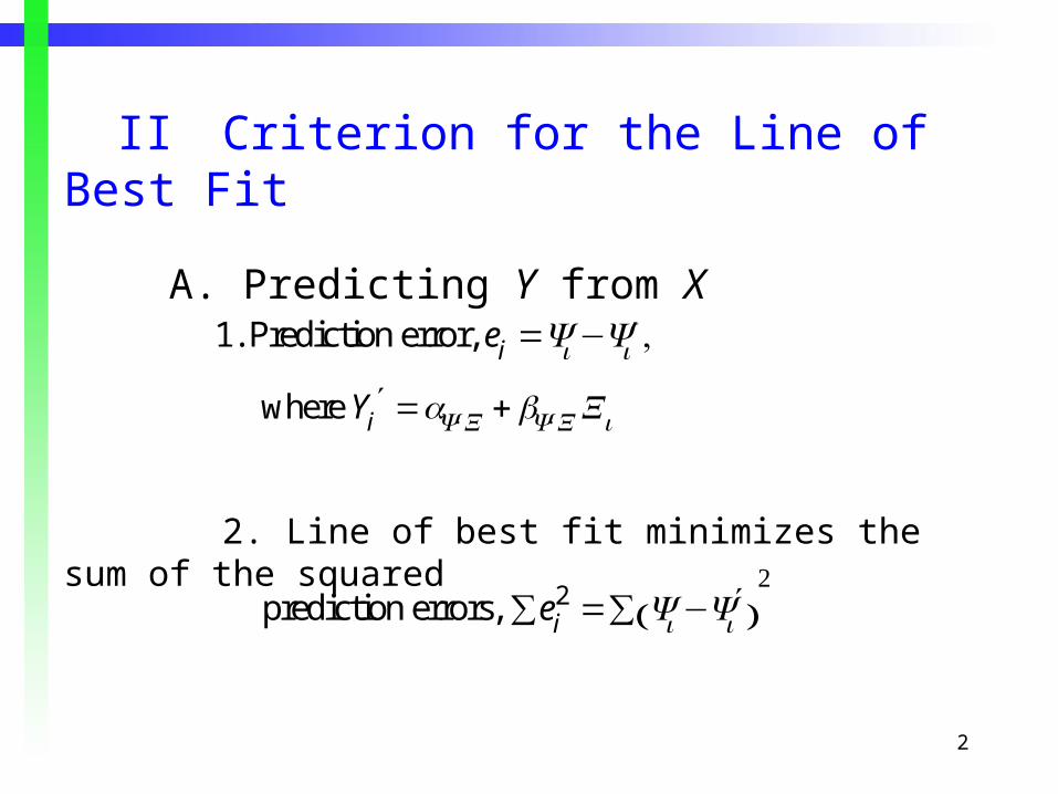
Table 1. Height and Weight of Girl’s Basketball Team

1 7.0 140 .64 289 13.62 6.5 130 .09 49 2.13 6.5 140 .09 289 5.14 6.5 130 .09 49 2.15 6.5 120 .09 9 –0.96 6.0 120 .04 9 0.67 6.0 130 .04 49 –1.48 6.0 110 .04 169 2.69 5.5 100 .49 529 16.1

10 5.5 110 .49 169 9.1

X i

Yi Girl ( X i −X)2

(Yi −Y )2

( X i −X)(Yi −Y )

(1) (2) (3) (4) (5)

X =6.2 Y =123 =2.10∑ =1610∑ =49.0∑

(6)

7

B. Computation of Line of Best Fit: Predicting Y from X

X = Xi / n=62.5 / 10 =6.2∑

Y = Yi / n=1230 / 10 =123∑

aY .X =Y −bY.X X =123−23.33(6.2) =−21.6667

bY .X =(Xi −X)(Yi −Y )∑

(Xi −X)2∑=49.02.10

=23.3333

8

1. Predicted weight for girl whose height is Xi = 6.5

Yi′ =aY.X +bY.X Xi

C. Predicting X from Y

X i′ =aX.Y +bX.YYi

bX .Y =(Xi −X)(Yi −Y )∑

(Yi −Y )2∑=49.01610

=0.0304

aX .Y =X −bX.YY =6.2−0.03(123) =2.4565

=−21.67 + 23.33(6.5) =130

9

1. Error in predicting X from Y

10

2. Predicted height for girl whose weight is Yi = 130

X i′ =aX.Y +bX.YYi

=2.46 + 0.03(130) =6.36

D. Comparison of Two Regression Equations

Yi′ =aY.X +bY.X Xi

=−21.67 + 23.33Xi

X i′ =aX.Y +bX.YYi

=2.46 + 0.03Yi

11

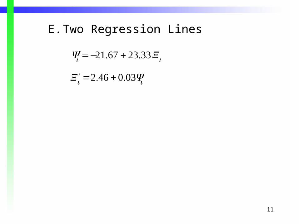
′Yi =−21.67 + 23.33Xi

′Xi =2.46 + 0.03Yi

E. Two Regression Lines

12

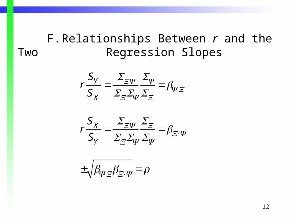
F. Relationships Between r and the Two Regression Slopes

r

SY

SX

=SXY

SXSY

SY

SX=bY.X

± bY.XbX.Y =r

r

SX

SY

=SXY

SXSY

SX

SY=bX.Y

13

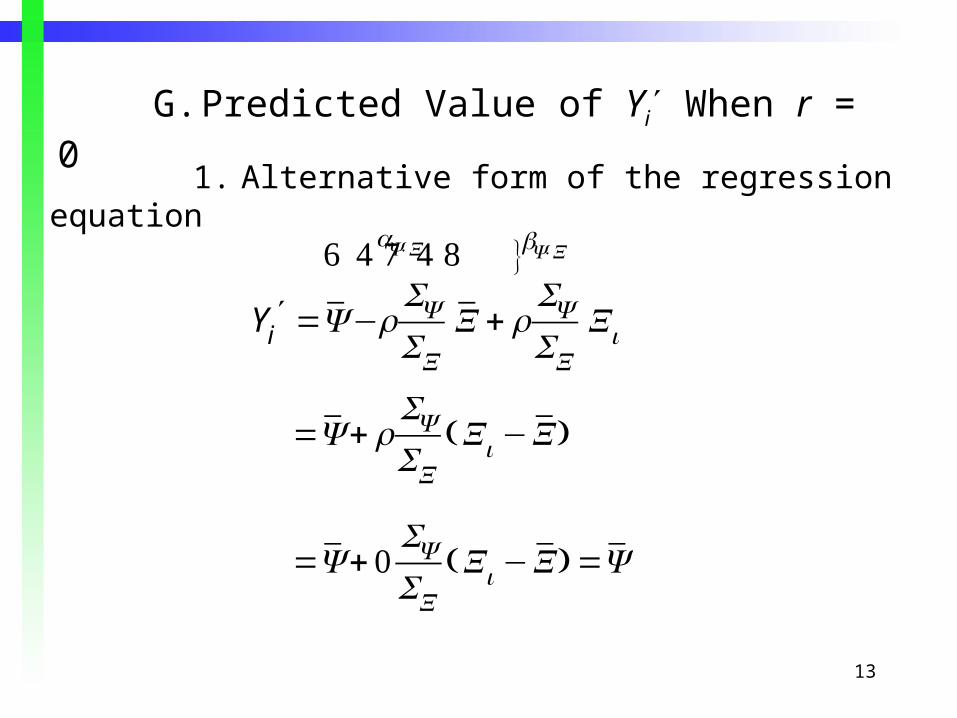
G. Predicted Value of Yi′ When r = 0

1. Alternative form of the regression equation

Yi′ =Y −r

SY

SXX

aY .X6 74 84

+ rSY

SX

bY .X}

Xi

=Y + r

SY

SX(Xi −X)

=Y + 0

SY

SX(Xi −X) =Y

14

III Standard Error of Estimate (SY.X)

A. Comparison of SY.X & Standard Deviation (S)

SY .X =

(Yi −Yi′)2∑

n S =

(Yi −Y )2∑n

Y

X

l

l

l

l

l

l

l

Y

X

l

l

l

l

l

l

l

15

B. Alternative Formula for SY.X

SY .X =SY 1−r2

1. Maximum value of SY.X occurs when r = 0

SY .X =SY 1−(0)2 =SY

2. Minimum value of SY.X occurs when r = 1

SY .X =SY 1−(1)2 =0

16

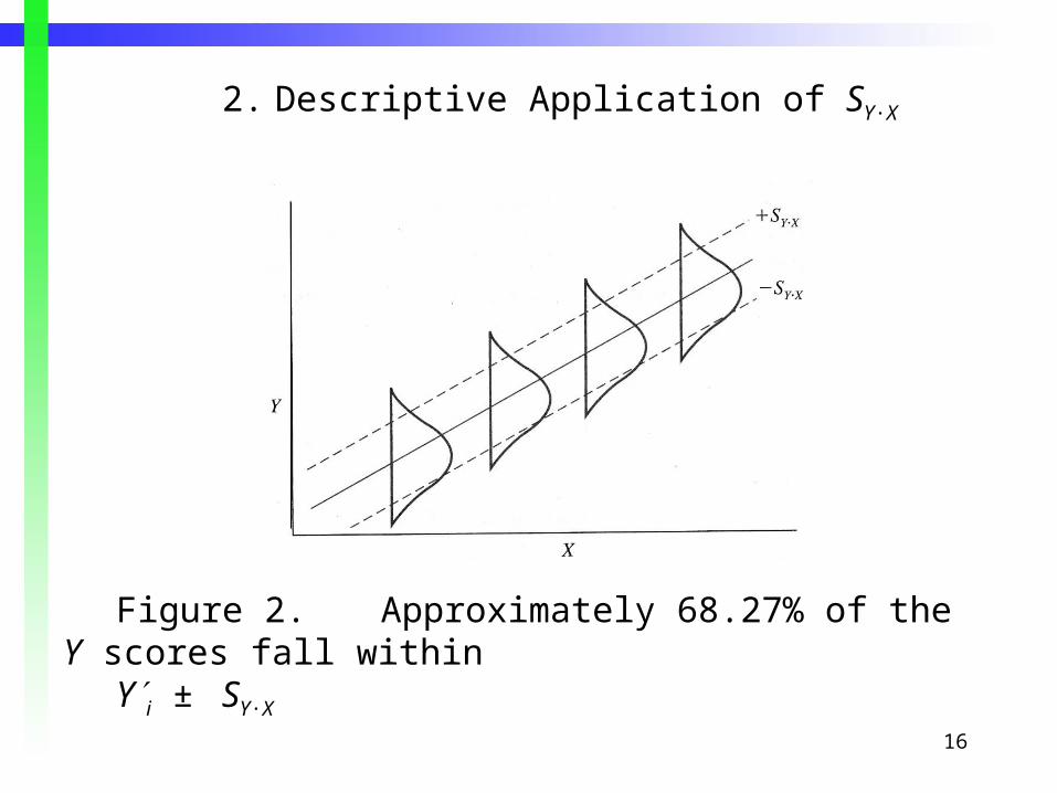
2. Descriptive Application of SY.X

Figure 2. Approximately 68.27% of the Y scores fall withinY′i ± SY.X

17

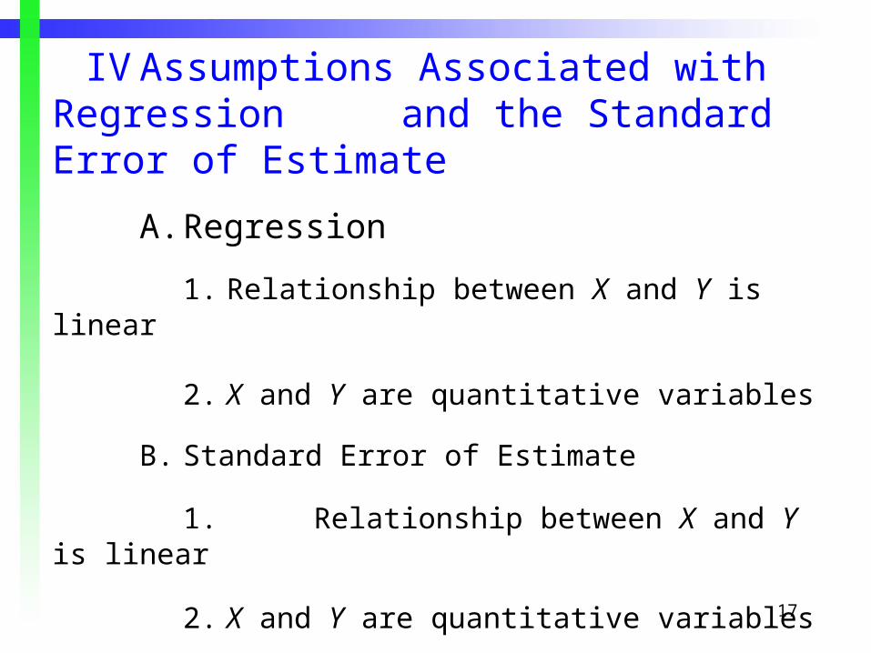
IV Assumptions Associated with Regression and the Standard Error of Estimate

A. Regression

1. Relationship between X and Y is linear

2. X and Y are quantitative variables

B. Standard Error of Estimate

1. Relationship between X and Y is linear

2. X and Y are quantitative variables

3. Homoscedasticity

18

V Multiple Regression

A. Regression Equation for k Predictors

′Yi =a+b1Xi1 +b2Xi2 +L +bkXik

B. Example with n = 5 Subjects and k = 2 Predictors

19

Table 2. Multiple Regression Example with Two Predictors

Observed Predictor Predictor Predicted Prediction Subject Score One Two Score Error__________________________________________________

1 3 4 3 3.90 -0.902 1 2 6 1.02 -0.023 2 1 4 1.70 0.304 4 6 5 3.75 0.255 6 5 1 5.63 0.37

___________________________________________________

(1) (2) (3) (4) (5) (6)

20

C. Multiple regression equation

′Y =a+b1Xi1 +bi2Xi2

=3.58 + 0.53Xi1 + (−0.60)Xi2

D. Simple Regression Equations

′Y =a+bXi1

=0.605+ 0.721Xi

′Y =a+bXi2

=6.230 + (−0.797)Xi

21

Table 3. Correlation Matrix for Data in Table 1______________________________________

Variable

Variable Y X1 X2

______________________________________

Y 1.000 .777 –.797 X1 1.000 –.338 X2 1.000______________________________________

22

Y

X2

1

2

3

4

6

1

2

3

5

4

5

1

2

3

4

5

6

•

•

•

•

a . b .

•

X1

•

•

Y

1

2

3

4

6

1

2

3

5

4

5

1

2

3

4

5

6•

•

•

X2

X1

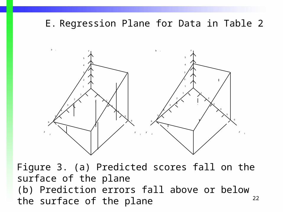
E. Regression Plane for Data in Table 2

Figure 3. (a) Predicted scores fall on the surface of the plane (b) Prediction errors fall above or below the surface of the plane

23

VI Multiple Correlation (R)

RY .X1X2=

rYX1

2 + rYX2

2 −2rYX1rYX2

rX1X2

1−rX1X2

2

A. Multiple Correlation for Data in Table 2

RY .X1X2=

(.777)2 + (−.797)2 −2 (.777)(−.797)(−.338)⎡⎣ ⎤⎦1−(−.338)2

=.962

24

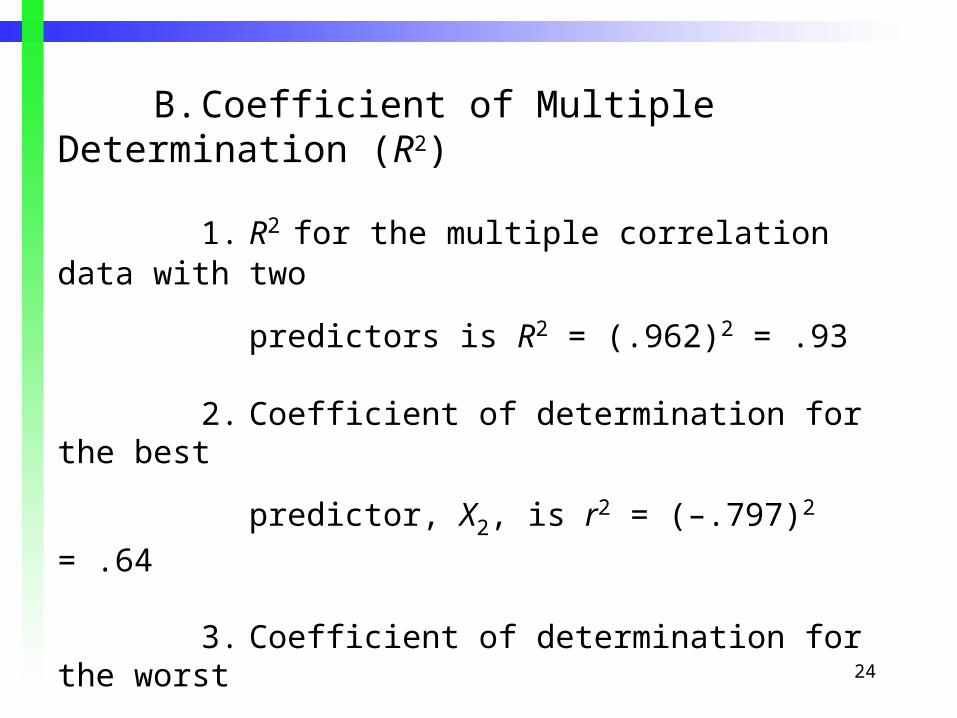
B. Coefficient of Multiple Determination (R2)

1. R2 for the multiple correlation data with two

predictors is R2 = (.962)2 = .93

2. Coefficient of determination for the best

predictor, X2, is r2 = (–.797)2 = .64

3. Coefficient of determination for the worst

predictor, X1, is r2 = (.777)2 = .60

C. The problem of multicollinearity