88

CHAPTER 6: CYCLONE RISKS Ken Granger, Bruce Harper, Trevor Jones, John Stehle, Matt Hayne and Jeff Callaghan

The Cyclone Threat There is little doubt that tropical cyclones pose a significant overall threat to Mackay. Since the settlement was founded in 1862 there have been at least 77 cyclones that have had an impact on the city. The greatest impact was caused by the cyclone of 21 January 1918, in which the combined effects of strong winds, storm tide and flood destroyed or damaged around 75% of the buildings in the town and took at least 30 lives. The inventory of cyclones affecting Mackay (Appendix M) is based largely on a listing of historical events compiled from many sources by the Bureau of Meteorology’s Queensland Regional Office in Brisbane. Of the 77 cyclones or ex-cyclones included in Appendix M, 19 have either crossed, or approached, the coast within 75 km of Mackay. A further 29 cyclones have approached to between 75 and 150 km of the city, with the remaining 29 being more distant than 150 km. An approach to within 75 km would bring Mackay within the radius of destructive winds of most cyclones of Category 2 or above.

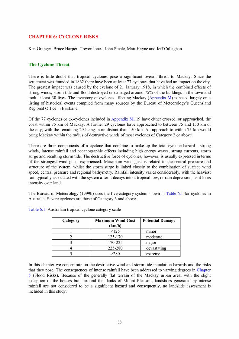
There are three components of a cyclone that combine to make up the total cyclone hazard - strong winds, intense rainfall and oceanographic effects including high energy waves, strong currents, storm surge and resulting storm tide. The destructive force of cyclones, however, is usually expressed in terms of the strongest wind gusts experienced. Maximum wind gust is related to the central pressure and structure of the system, whilst the storm surge is linked closely to the combination of surface wind speed, central pressure and regional bathymetry. Rainfall intensity varies considerably, with the heaviest rain typically associated with the system after it decays into a tropical low, or rain depression, as it loses intensity over land. The Bureau of Meteorology (1999b) uses the five-category system shown in Table 6.1 for cyclones in Australia. Severe cyclones are those of Category 3 and above. Table 6.1: Australian tropical cyclone category scale

Category Maximum Wind Gust (km/h)

Potential Damage

1 <125 minor 2 125-170 moderate 3 170-225 major 4 225-280 devastating 5 >280 extreme

In this chapter we concentrate on the destructive wind and storm tide inundation hazards and the risks that they pose. The consequences of intense rainfall have been addressed to varying degrees in Chapter 5 (Flood Risks). Because of the generally flat terrain of the Mackay urban area, with the slight exception of the houses built around the flanks of Mount Pleasant, landslides generated by intense rainfall are not considered to be a significant hazard and consequently, no landslide assessment is included in this study.

89

The Cyclone Phenomenon The strict definition of a tropical cyclone (WMO, 1997) is:

A non-frontal cyclone of synoptic scale developing over tropical waters and having a definite organized wind circulation with average wind of 34 knots (63 km/h) or more surrounding the centre.

Basically, the tropical cyclone is an intense tropical low pressure weather system where, in the southern hemisphere, winds circulate clockwise around the centre. In Australia, such systems are upgraded to severe tropical cyclone status (referred to as hurricanes or typhoons in some countries) when average, or sustained, surface wind speeds exceed 120 km/h. The accompanying shorter period destructive wind gusts are often 50 per cent or more higher than the sustained winds. Tropical cyclone development is complex, but various authors (including Gray, 1975; Riehl, 1979 and WMO 1995), have identified six general parameters necessary for their formation and intensification. Dynamic parameters include low-level relative vorticity, exceedence of a threshold value of the Coriolis effect of the earth’s rotation, and minimal vertical shear of the horizontal wind between the upper and the lower troposphere. Thermodynamic parameters include sea surface temperature (SST) above 26°C through the mixed layer to a depth of 60 m, moist instability between the surface and the 500 hPa level (approximately 5600 m above sea level), high values of middle tropospheric relative humidity, and warm upper troposphere air. Globally, tropical cyclones form more frequently in the Northern Hemisphere (with 75% of the global total) than in the southern hemisphere (Gray, 1968 and 1979). In the southern hemisphere, cyclones occur in three principal regions: the Indian Ocean near Madagascar, where over 10% of the global total cyclones occur; the oceanic area to the northeast and northwest of Australia; and in the Gulf of Carpentaria. Cyclones in the Australian region occur predominantly between 15° and 20°S, commencing in November/December and continuing to March/April. The greatest incidence is in January to March, transferring from east to west as the season advances (Lourensz, 1981). In terms of both cyclone intensity and the likelihood of crossing the coast, the most cyclone-prone area along the Queensland coast is around Mackay (Harper, 1998). The period of recorded observations of cyclone occurrences, however, is only a little more than 100 years. In sparsely settled regions or regions remote from the coast, the records are accurate only since the advent of satellite observation from the early 1960s. Once formed, cyclones in the Southern Hemisphere tend to move westwards and polewards under combined easterly steering currents and dynamic effects, although individual tracks can be erratic. Cyclonic movement along the Queensland coast between 10° and 15°S latitude is mostly southwest to westward and south to southeastward. South of latitude 15°S, the major direction of movement is southeastward (Coleman, 1971) due to interaction with predominantly westerly flows. Continental east coast effects also tend to cause blocking and steering such that many cyclones tend to track southwards parallel to the coast. The main structural features of a severe tropical cyclone are the eye, the eye wall and the spiral rainbands. The eye is the area at the centre of the cyclone at which the surface atmospheric pressure is lowest. It is typically 20 to 50 km in diameter, skies are often clear and winds are light. The eye wall is an area of cumulonimbus clouds which swirls around the eye. Studies by Black and Marks (1991) and Wakimoto and Black (1994) suggest that unusually high winds can occur in the vicinity of the eye wall due to instabilities as the cyclone makes landfall. Tornado-like vortices of even more extreme winds may also occur in association with the eye wall and outer rain bands. Tornadoes on the outskirts of

90

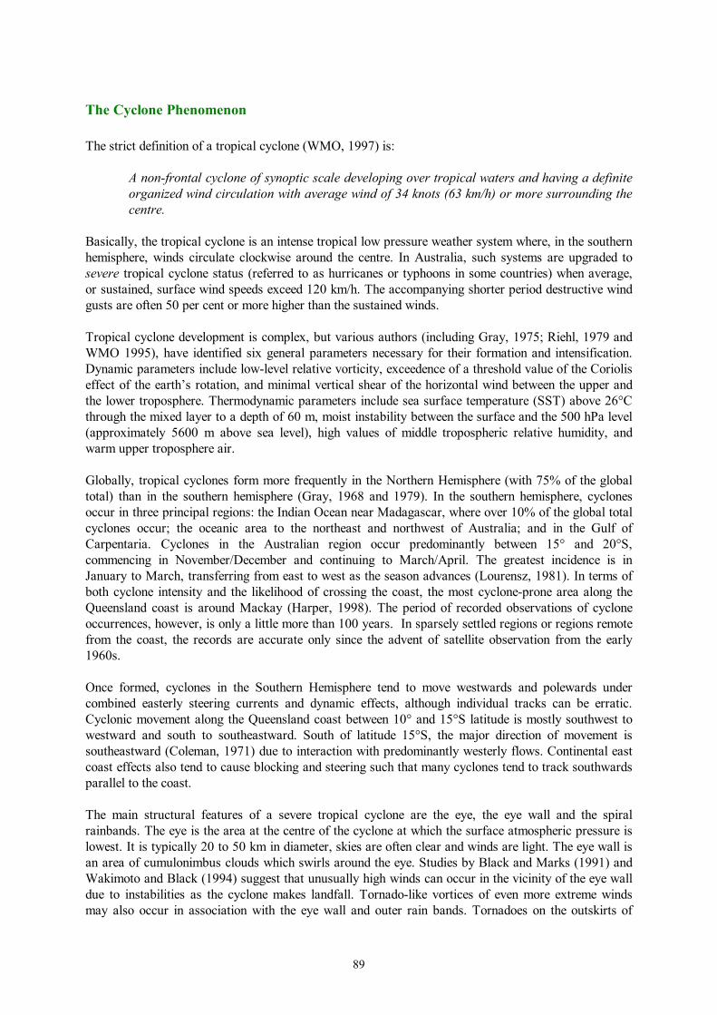
tropical cyclones have been experienced in Mackay on at least three occasions. The rain bands spiral inwards towards the eye and can extend over 1000 km or more in diameter. The heaviest rainfall and the strongest winds, however, are usually associated with the eye wall. Given specifically favourable conditions, tropical cyclones can continue to intensify until they are efficiently utilising all of the available energy from the immediate atmospheric and oceanic sources. This maximum potential intensity (MPI) is a function of the climatology of regional sea surface temperature (SST) and atmospheric temperature and humidity profiles. Applying a thermodynamic MPI model (Holland, 1997) for the Mackay region, the MPI is thought to represent a central pressure of about 895 hPa. This is considerably more intense than any cyclone to date recorded in the region but not as low as has been experienced worldwide. Thankfully, it is rare for any cyclone to reach its MPI because environmental conditions often act to limit intensities in the Queensland region. The windfield within a moving cyclone is generally asymmetric so that, in the Southern Hemisphere, winds are stronger to the left of the direction of motion of the system (the ‘track’). This is because the direction of cyclone movement and circulation on the left-hand side of the cyclone act together; on the right-hand side they are opposed. During a coast crossing in the Southern Hemisphere, the cyclonic wind direction is onshore to the left of the eye (seen from the cyclone) and offshore to the right. For any given central pressure, the lateral extent of individual tropical cyclones can vary enormously. Examples of the surface pressure (isobar) fields of two very different tropical cyclones that have affected Mackay are shown in Figure 6.1. The first is that of Ada in 1970, which devastated the Whitsunday Islands region 80 km to the north. This was a particularly small cyclone with modest central pressure, but it was embedded in a relatively high pressure zone and produced extreme winds. It was so small that the zone of destructive winds fitted between the coast and the Great Barrier Reef. The alternative example is Justin in 1997. Justin was a very large cyclone centred more than 500 km north of Mackay. This storm, again with modest central pressure at the time, generated extreme waves and a persistent storm surge over many days causing extensive coastal damage. Coastal damage was due to the alignment of the outer winds with the exposed eastsoutheast fetch near Mackay, which is not protected by the Great Barrier Reef.

1200 UTC Jan 1970 Ada (963 hPa) 0000 UTC Mar 1977 Justin (978 hPa) Figure 6.1: Examples of tropical cyclones affecting the Mackay region (surface isobars shown in

91

2 hPa intervals)

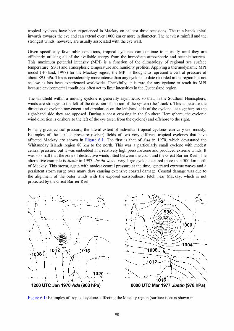
The Mackay Cyclone Experience The cyclone season in Mackay is typical of the Southern Hemisphere, extending from late November to April, with the occasional event occurring in May. The greatest incidence of cyclones occurs during January, February and March. Figure 6.2 shows February to be the month in which, historically, more of the close cyclones occur; January, February and March have more of the mid-distance cyclones; and January has more of the distant cyclones.

0

5

10

15

20

25

December January February March April May

Months

Num

ber o

f cyc

lone

s

150-300 km

75-150 km

0-75 km

Figure 6.2: Frequency of cyclones in the Mackay area 1867-1997. Of the 77 cyclones that have had some effect on Mackay (listed in Appendix M), at least ten have inflicted substantial damage other than flooding (covered in Chapter 5) or caused significant dislocation. A brief outline of these events and their impact will provide some level of appreciation. It is difficult, however, to make direct comparisons of damage between individual cyclones because the Mackay township has changed greatly over time. The ten most notable cyclones were:

• 17 February 1888 – an unnamed severe cyclone recurved near Mackay with severe winds destroying several buildings. One ship was lost and another dismasted;

• 4 February 1898 – Cyclone Eline recurved very close to Mackay causing extensive destruction and flooding. The court house and two churches were destroyed and many other buildings were damaged;

• 10 December 1915 – winds from an unnamed low category cyclone, tracking from the north, bent telegraph poles and damaged roofs in the town;

• 21 January 1918 – an unnamed, at least Category 4 cyclone, scored a bulls eye hit on Mackay bringing with it a 3.6 m storm surge that inundated much of the town to a level of 5.4 m above AHD. The storm tide and the winds destroyed around 1200 buildings and damaged most of the rest. At least 30 people lost their lives;

92

• 7 March 1955 – an unnamed Category 3 cyclone crossed the coast at Sarina to the south. Widespread wind damage was experienced in Mackay;

• 17 January 1970 - small Category 3 Cyclone Ada passed through the Whitsunday Group and within 80 km from the city at its closest point. Severe damage was experienced in the area close to the track and the Pioneer River reached major flood levels.

• 5 March 1976 – Category 1 Cyclone Dawn crossed the coast within 30 km of Mackay. Two houses were unroofed in North Mackay;

• 1 March 1979 – Category 1 Cyclone Kerry crossed the coast at Proserpine, 80 km to the north. Significant wind damage was suffered by at least 26 houses in Mackay and many boats were destroyed by huge seas inside the outer harbour;

• 26 December 1990 – Category 4 Cyclone Joy, which had weakened to Category 2 level by the time it reached Mackay, caused extensive damage. A tornado demolished two houses and damaged at least 40 others. A seaside caravan park was extensively damaged by high seas and one person drowned in the surf;

• 9 March 1997 – Category 4 Cyclone Justin had not reached its full strength when it generated massive seas that caused significant coastal erosion on all of Mackay’s beaches.

The full text of the description of the 1918 cyclone, published in the Mackay Daily Mercury on 26 January 1918 (five days after the disaster), is contained in Appendix N, along with other contemporary reports of the cyclone. Some of the key observations include:

The destructive period of the cyclone was about ten hours and it was almost incredible the amount of damage that was done in that short period [Plate 6.1]. Some of the residents are able to report that not a pane of glass was damaged in their homes, but they are very few. Of the 1200 or 1400 houses within the Municipality of Mackay, not more than one quarter escaped damage of some kind, and in a great many cases the buildings were levelled to the ground. The town on Monday afternoon presented an appalling spectacle. The damage in most cases consisted of the houses being unroofed, and this particularly applied to the larger buildings such as hotels, churches, public halls and two-storied buildings [Plate 6.2 and Plate 6.3]. As with other classes of buildings some of them collapsed entirely and some sustained partial damage only. The residential area suffered severely. A great many of the residences were thrown down and completely destroyed, while others were unroofed or otherwise damaged. No particular part of the town suffered more than any other part. The damage was general in town and country and confirms the opinion that the centre of the cyclone traversed the district…..

While the cyclone was at its height another terror, in the shape of a tidal wave, swept the town and caused consternation amongst the fear wracked householders. It struck the coast about five o'clock when the cyclone was raging and it is alleged a wall of water 25 ft [7.6 m] high swept over the beaches; and taking a southwesterly direction submerged the town to varying depths as far out as Nebo Road. It was 5 or 6 ft deep on Beach Road and about 2 ft deep at the Ambulance corner. The water flowed inland in waves, carrying debris of a substantial character with it. In the river the wave played havoc with the shipping, wharves, stores and houses, while a large section of the Sydney Street bridge, which is the main avenue between Mackay and North Side, was washed away…. The heavy rain, combined with the big tide, caused a record flood in the river on Tuesday. There is no authentic record as to the height the river rose, as the gauges were all washed away, but the Harbour Master (Captain Greenfield) states that the water rose at least 20 ft. The lower portion of the town was inundated to a depth of [unreadable]. The river broke across below Devil's Elbow into Barnes Creek and relieved the pressure in the main outlet, and on Thursday morning the back water in the land near the cemetery overflowed and crossing Nebo Road, rushed down Shakespeare Street and a parallel street to a depth of 3 ft. It is the opinion of experienced men that

93

had this second diversion not occurred the loss of life would have been enormous. The flood commenced to subside on Thursday afternoon and is already back to normal…. Mr J. Shanks and his brother Mr Frank Shanks, also had a terrible experience. They resided in the old butter factory and when the tidal waters entered the building took refuge in what they considered the strongest room in the house and put their wives and families on a table. The water rose above the level of the table and another one was placed on top and as the waters still continued to rise chairs were provided. When everything seemed secure, the kitchen from the house adjoining collapsed and partly demolished the building where the people were. Mr Frank Shanks was rendered insensible through being struck by falling timber and all were thrown into the water. Mr J. Shanks then heroically secured rafts and ultimately, after a fierce battle with the elements, and a most perilous journey, during which his wife and children and his brother's baby disappeared, he reached the Waterside Workers Hall and gained entrance through a window. Mr Frank Shanks afterwards reached Tennyson Street and upon his information a rescue party was organised and a number of people, including Mr. and Mrs. Weir and several who had sought refuge in their residence, together with those who were in the hall, were rescued. The force of the rain was terrible, Mr Shanks remarking that he was bruised all over with the driving rain and had every stitch of clothing ripped off his body.

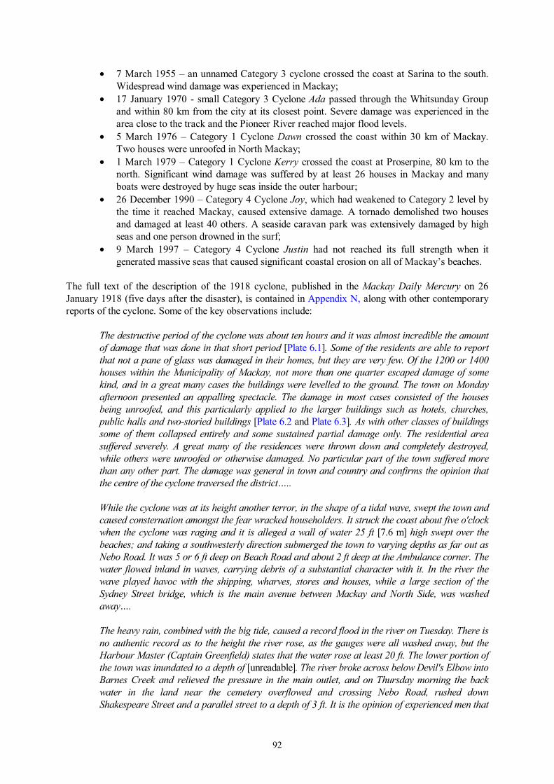
Parkinson and others (1950) mapped the extent of storm tide inundation produced by the 1918 cyclone. This, together with the location of known fatalities in the Mackay urban area, is shown in Figure 6.3. In all, at least 30 people died in the cyclone of which 13 drowned in the storm tide and two died due to buildings collapsing. The numbers of dead at each location is shown in the figure. It is little wonder that the Mackay community still takes the threat of cyclones more seriously than most other communities in Queensland.

94

Figure 6.3: Mackay 1918 storm tide inundation and number of fatalities

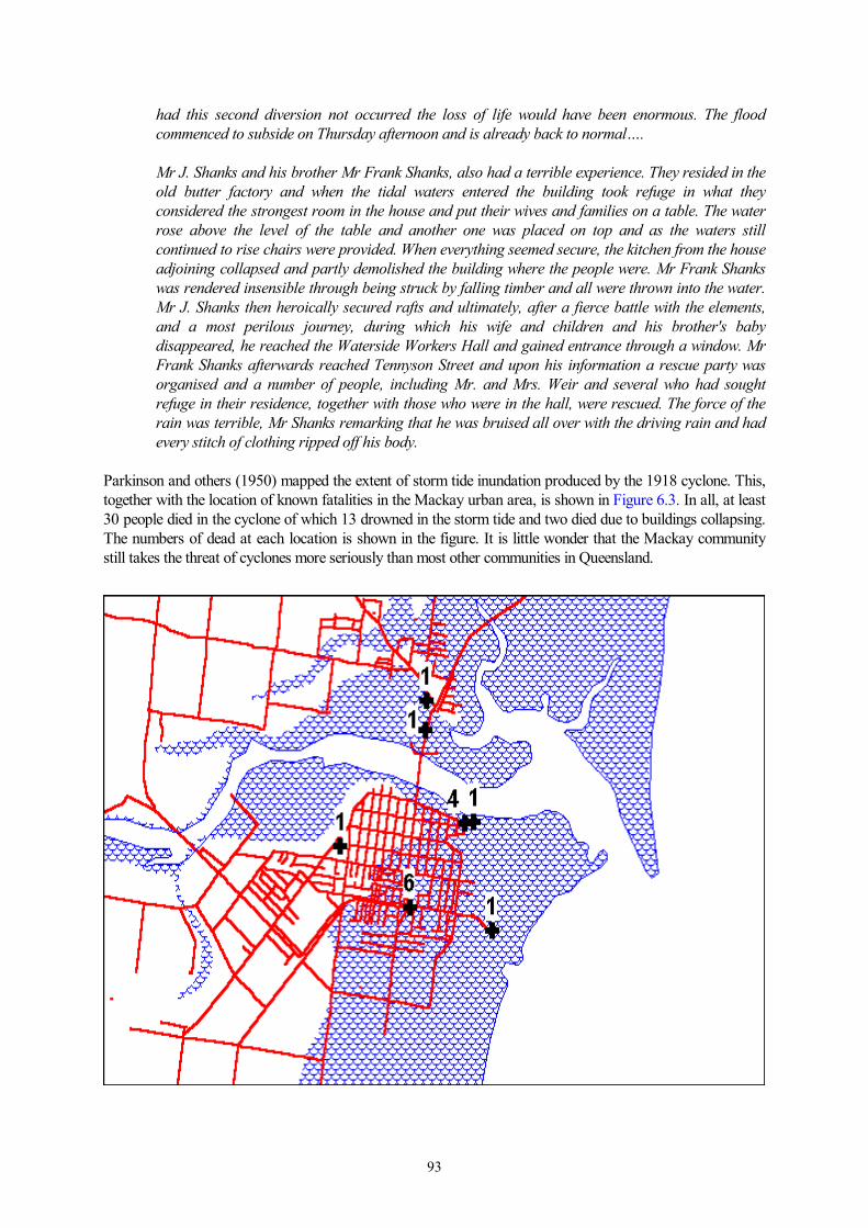
Cyclone Variability Observational record: Holland (1981), observed that tropical cyclone data are only as good as their concomitant observing systems and analysis techniques. The most common flaw in tropical cyclone records is missing data. In Australia, for example, the number of recordings increased from 1909 to 1959, parallel with an increase in population and trade in the north of the continent (Holland, 1981). It was not until 1966, with the launching of ESSA satellites, that cyclones could be investigated systematically. Based purely on observational records, Ryan (1993) noted that cyclonic frequency varied considerably in the Australian region between 1959 and 1989, from five cyclones in 1988-1989 to a maximum of 19 in 1963-1964, however, no trend is apparent. Yearly cyclonic frequency near Mackay has been calculated using cyclones which track within 300 km of the site and for which an impact has been recorded (Figure 6.4). Cyclonic frequency shows considerable variability and although there is a trend suggesting an increase in frequency towards the present this is thought to be due to incomplete data sets as mentioned above. For the reliable portion of the recorded period from 1966 to present, the record shows considerable variability with three cyclones occurring in 1976.

Figure 6.4. Yearly occurrences of tropical cyclones within 300 km and impacting on Mackay Climatic Variability: Figure 6.4 shows that the incidence of tropical cyclones can be quite variable from one year to the next. This is because of the complex set of factors which influence their genesis (WMO 1995). For many years one of the principal indicators of seasonal cyclonic activity has been the so-called El Niño - Southern Oscillation (ENSO) phenomenon. This is the name given to a quasi-biennial (between one and three year) cycle of alternating cold and warm ocean temperatures between one side of the Pacific Ocean and the other. The El Niño phase sees abnormally warm ocean temperatures off the

0

1

2

3

4

1860 1880 1900 1920 1940 1960 1980 2000

Years

Num

ber o

f cyc

lone

s

95

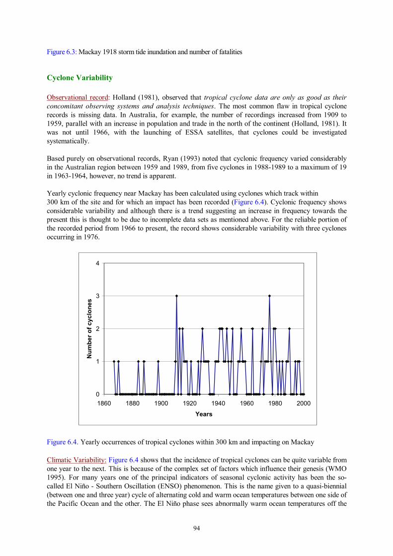
coast of South America and along the central and eastern Pacific equatorial zone and simultaneously cooler ocean temperatures in the western Pacific and the Coral Sea. During the reverse cycle, or La Niña, ocean temperatures near Mackay are typically above average. Ocean temperature is not the only factor causing cyclone variability but it is a prime contributor, and, when combined with associated shifts in large-scale zones of atmospheric convergence (Basher and Zheng, 1995), the regions of tropical cyclone genesis in the South Pacific tend to move further towards the east (El Niño) or west (La Niña) during ENSO events. Several techniques are used to determine the state or strength of the ENSO condition. One of the most widely used methods is the Southern Oscillation Index (SOI), which compares differences in the mean monthly sea level pressure between Darwin and Tahiti. The SOI has been shown to be a strong indicator of rainfall and tropical cyclone activity in northern Australia and Queensland (e.g. Nicholls, 1992). Another common method is to use SSTs from various zones in the Pacific. These data have become routinely available from satellite as well as ships, drifting buoys and from moored buoy networks positioned along the equator. Using an accepted SST-based sequence from 1959 to 1997 (e.g. from Pielke and Landsea, 1999), Figure 6.5 shows that when the historical record is separated into El Niño and La Niña periods, there is a noticeable effect on the tracks of tropical cyclones in the Coral Sea. During La Niña (the positive SOI phase) cyclone activity tends to be located closer to the east coast of Queensland than during the El Niño (negative SOI phase). While the ENSO phenomenon appears to be somewhat random, El Niño years have outnumbered La Niña years by about a factor of three since the mid-1970s. This has been reflected along much of the east coast of Queensland by a corresponding reduction in frequency of cyclone occurrence and Figure 6.4 indicates this effect from about 1980 onwards within 300 km of Mackay. Exactly why this preference for El Niño episodes has persisted during this period is not entirely clear but it may be related to longer period climatic variability as discussed in the next section, or even global climate change. From 1998 to early 2000 there has been a return to mild La Niña and near-neutral conditions. Figure 6.5. Differences in tropical cyclone tracks between El Niño (left) and La Niña (right) years. Power and others (1999) recently highlighted the potential importance for the Australian climate of an apparent 10 to 30 year longer-term cycle of ocean temperatures in the Pacific Ocean. This oscillation is also measured in terms of relative SST heating or cooling but relates more to the whole of the tropical Pacific Ocean region rather than just differences between the eastern and western limits. Termed the Inter-decadal Pacific Oscillation (IPO), this long-term variation in mean SST appears to modulate the effect of ENSO on rainfall in Australia. When the IPO is “positive”, the tropical ocean is slightly warmer than average while to the north and south the temperatures are slightly less than average.

Cairns •

Weipa •

Cooktown •

Townsville •

Mackay •

Gladstone •

Noosa •Brisbane •

Ballina •

140ºE 150ºE 160ºE

30ºS

20ºS

10ºS

Cairns •

Weipa •

Cooktown •

Townsville •

Mackay •

Gladstone •

Noosa •Brisbane •

Ballina •

140ºE 150ºE 160ºE

30ºS

20ºS

10ºS

96

During this period the effect of ENSO on rainfall appears to be less significant. When the IPO is “negative”, the tropical ocean is slightly cooler and ENSO seems to be much more strongly correlated with Australian rainfall. The IPO effect may also be related to the large-scale thermo-haline circulation between the Atlantic and the Pacific Ocean that has been identified as a potential indicator of hurricane incidence in the Atlantic (Landsea and others, 1994). Callaghan and Power (under review) describe a possible modulating effect of the IPO on Australian tropical cyclone activity which suggests that damaging impacts in Queensland are more likely during negative (cooler) phases of the IPO, which is associated with warmer ocean temperatures near Queensland. Again, since the mid-1970s, there has been a prolonged positive phase of the IPO that is only now (1999-2000) showing some possible signs of reversal. If this is correct, recent trends may suggest that cyclone incidences along the Queensland coast could increase. Climate Change: The potential impact of global warming arising from the so-called “enhanced Greenhouse effect” has become a major scientific and social issue since the 1980’s. Greenhouse warming occurs when solar radiation absorbed by the earth is re-emitted as heat energy back into the atmosphere where it is partly trapped by “greenhouse” gases. These gases then re-emit the radiation in all directions, further warming the atmosphere and the earth’s surface. The process is a natural one; without these gases the earth’s surface would be approximately 33oC cooler. However, human activities are believed to have markedly increased the level of greenhouse gases such as CO2 and CFC’s in the atmosphere. This is expected to raise global temperatures over time, potentially leading to changed climates. One of the consequences of these changes could be a change in the incidence, severity and southern movement of tropical cyclones. A global “consensus” report on climate change is provided by the Intergovernmental Panel on Climate Change (IPCC) of the World Meteorological Organisation (WMO) and United Nations Environment Program (UNEP). It is updated at approximately five-year intervals, following an intensive review by some hundreds of scientists. According to the IPCC Second Assessment Report in 1995 (IPCC, 1996):

• the climate has changed over the past century; • the balance of evidence suggests a discernible human influence on global climate; • the climate is expected to continue to change in the future; • there are still many uncertainties, including the rates and regional patterns of climate change; • there is a possibility for more extreme rainfall events; • there could be enhanced precipitation variability associated with ENSO; • under the “business as usual” emissions scenario, sea level is expected to rise by between 20 cm

and 86 cm, with a best estimate of about 50 cm, by 2100; and, • global mean surface air temperature is expected to rise between 1oC and 3.5oC, with a best

estimate of 2oC, by 2100. Substantial regional variations in these estimates are to be expected. IPCC (1996) highlights the uncertainties in past data records of tropical cyclones and the difficulties in discerning any long-term trends, but suggests that there may be an increase in cyclone frequency and intensity. More recently, Henderson-Sellers and others (1998) presented an expert consensus that concedes the possibility of a modest increase in the maximum potential intensities of tropical cyclones but with little likelihood of increased frequency or coverage. Given the possible implications of future climate change scenarios, it could be prudent in Mackay to plan for a possible increase in the intensity of cyclones as compared with the last 25 year period. Interpreted record: A different approach to the interpretation of cyclonic frequency uses evidence from storm surge deposits. This method can produce frequency records dating back 6500 years, highlighting longer period variability as well as bypassing the problems associated with observational records.

97

Hopley (1968) was one of the first to interpret storm ridge patterns in northern Australia. Hopley inferred a mid to late Holocene change of storm intensity and direction from the morphology of early versus late shingle deposits at Curacoa Island (350 km northwest of Mackay). Hopley, suggested that at the time of initial spit formation (about 6000 radiocarbon years B.P.), the dominant waves had a greater northerly or northeasterly component and that stormier conditions prevailed. Later, Rhodes (1980) established a radiocarbon dated record of Holocene storm ridges at western Cape York Peninsula. According to Rhodes, there were four periods of ridge development, the earliest between 5900 and 4700 years B.P., the second between 3500 and 2500 years B.P., the third around 1400 years B.P. and the last from 400 B.P. to the present. Rhodes also analysed 25 radiocarbon ages collected by Smart (1976) from Cape Keer Weer on western Cape York Peninsula and considered that they showed ridge formation during approximately the same four periods. Chappell and others (1983) suggested that patterns of cyclone frequency could be deduced from storm ridge sequences in north Queensland, on the basis of data from Curacoa Island (northeast of Townsville) and other sites. Radiocarbon dates from the past 4000 years were grouped into 500 year intervals and the assumption that cyclone frequency has not changed was tested statistically. Further in-depth analysis by Hayne and Chappell (in press) at Curacoa Island and Princess Charlotte Bay beach ridge sequences, found no significant variation of cyclone frequency at either site for the past 6000 years and 2500 years respectively. A similar study is reported by Chivas and others (1986) from Lady Elliot Island in the southern Great Barrier Reef. Dates from beach ridge samples appear to show that there has been no significant variation of ridge-building event frequency during the past 4000 years (Chappell and Thom, 1986; Chivas and others, 1986).

Cyclone Warning Systems The Bureau of Meteorology Tropical Cyclone Warning Centre (TCWC) in Queensland, based in Brisbane, has responsibility derived from The Meteorology Act (1955) for issuing warnings of tropical cyclones which might affect the Queensland coast (Bureau of Meteorology 1999c). This encompasses an area essentially between 138oE (Gulf of Carpentaria) and 160oE (west of New Caledonia). A continuous watch is maintained over this area for the possibility of a tropical cyclone entering or developing. Once developed, the TCWC is responsible for naming the system using an internationally approved sequence of names. The TCWC then monitors and predicts the intensity, structure and movement of any tropical cyclone within its jurisdiction. The TCWC has an array of informational and computational resources used by its staff. These include an extensive network of automatic weather stations (AWS), 15 of which are located along or offshore of the Great Barrier Reef between 15oS and 25oS providing a very effective observational system. Additionally, weather radars provide coverage within about 300 km of the entire east coast south of 15oS. A variety of satellite derived products are also available (visible and infra-red imagery, radar and water vapour), and guidance is provided from a number of numerical weather models, both global and for the local area. Ranges of warning products are produced depending on the situation. Tropical Cyclone Outlooks are disseminated daily to advise the potential for cyclonic activity within 72 hours. A Tropical Cyclone Information Bulletin is issued whenever a tropical cyclone exists but is not posing a threat to the coast. A Cyclone Watch is issued if coastal or island communities are expected to be affected by gales within 48 hours. This is upgraded to a Cyclone Warning if gales are expected within 24 hours. Tropical Cyclone Threat Maps are also issued at this time to indicate the extent of watch and/or warning zones

98

in relation to particular localities as well as showing the extent of gale force, storm force and hurricane force winds. Warnings are updated hourly during periods of significant community threat. Storm tide warnings are issued by the Bureau of Meteorology in conjunction with the State Counter Disaster Organisation (SCDO, 1994) which interfaces with a number of key State Government organisations. Department of Emergency Services (DES) provides the executive role for the SCDO. The Beach Protection Authority (BPA), now a part of the Environmental Protection Agency (EPA), provides specialist advice and data in respect of wave and storm surge readings from its real-time network of waverider buoys and storm surge gauges. The issuing of storm tide warnings is also staged depending on the threat and the expected onset of high winds at the affected locations, which might impede potential evacuation to higher ground.

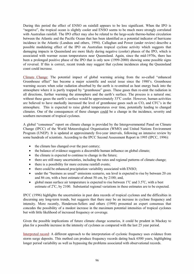
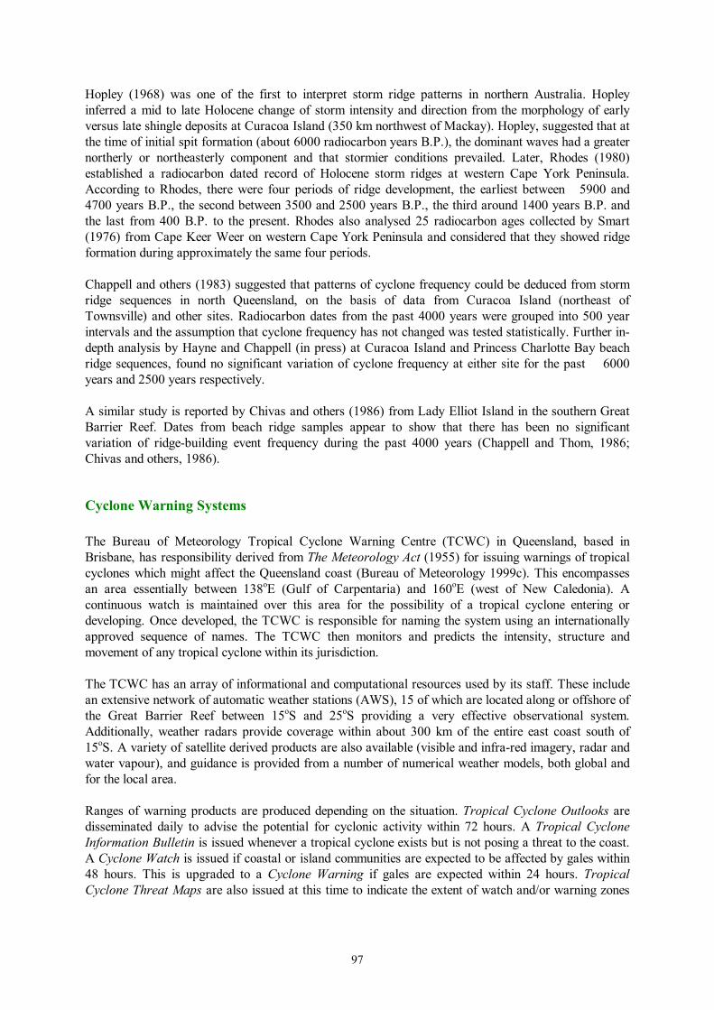
Severe Wind Risks Most of the structural damage caused by tropical cyclones is inflicted by the strong winds that reach their peak in the eye wall. This damage can be caused directly by the wind and/or by the debris that it propels, frequently with great force. Wind damage tends to increase disproportionately to the wind speed. According to Meyer (1997), winds of 70 m/sec (250 km/h) cause, on average, 70 times the damage of winds of 35 m/sec (125 km/h). Damage tends to start where sustained wind speeds begin to exceed 20 m/sec (about 75 km/h). In addition to the high wind speeds, the turbulence of the winds caused by terrain features and large buildings is also a decisive factor. Turbulence is often a particular problem on the lee slope of hills, such as Mount Bassett and Mount Pleasant. However, for the vast majority of the Mackay urban area, local terrain effects will be minimal. Buildings: The construction, design, age and location of buildings each have an influence on the risk of building damage. Advances made in cyclone resistant construction since the 1970s have resulted in improved building performance under wind loads. Generally, however, metal roofs are more susceptible to wind damage than are tile roofs, though the latter are more susceptible to damage by wind-driven debris; reinforced brick and concrete block walls are resilient, while fibro, metal cladding and even timber walls are susceptible to being penetrated by debris. Large areas of unprotected glass are even more susceptible to both wind and debris damage. Roof shape and pitch are influential. In simple terms, gable ended roofs take the full force of the wind, whereas the wind flows more smoothly over hip ended roofs. Depending on wind direction, flat or low pitched roofs can experience greater levels of suction than do high pitched roofs. Hip ended roofs with a pitch of around 30o tend to perform the best. The fastening of roofing material to trusses and the fastening of roof members to walls and foundations are also important. Some of the key forces on buildings are illustrated in Figure 6.6 and Figure 6.7. These are based on Meyer (op. cit. p.18). The first figure shows the way in which the suction forces generated on low pitched roofs may be countered by a reduced pressure inside the building where the integrity of the windward walls and windows are maintained and there is a predominance of openings on the leeward side. The second figure shows how an overpressure inside the building is created when that integrity is compromised by a window being broken on the windward side. The additional force can destroy the roof, if not the whole structure.

99

wind reducedpressure

Figure 6.6: Wind forces working on a building with external integrity

wind overpressure

Figure 6.7: Wind forces working on a building where its external integrity is lost Wind loading standards in Australia were first implemented by structural engineers in 1952. It was not until the experience of the severe destruction wrought by Cyclones Althea (Townsville) in 1971 and Tracy (Darwin) in 1974 that efforts were made to strengthen building standards in Queensland and elsewhere in Australia, especially for domestic structures termed “non-engineered structures”. Standard AS1170.2 Minimum design loads on structures: Part 2 – Wind loads was first published in 1973 and was subsequently revised in 1975, 1981 and 1983. The current (5th) edition was published in 1989 (Standards Australia, 1989). This Standard was first adopted under the Queensland Building Act in 1981, and had already become widely applied for domestic structures in Queensland by that time. AS1170.2-1989 is now encompassed by the Building Code of Australia. The wind loading code is based on a design event for which there is a 5% probability of exceedence in any 50 year period (i.e. a notional 1000 year ARI). The wind loading code makes some allowance for the site on which the building stands. Buildings on ridge crests, for example, are more exposed than are buildings on flat ground; buildings close to the coast or on open country are more exposed than buildings further inland or grouped in suburban settings. By-and-large, ridge crest terrain exposure is not a significant issue for wind hazards in the Mackay study area, however, some 7630 buildings (37% of the total) lie within one kilometre of the shoreline and the open land of the airfield. Building age is highly significant because it reflects both the degree of conformance to the Building Code, and the degree to which factors such as metal fatigue and the corrosion of metal fixings may have progressed. Mahendran (1995), for example, reported that exposure of metal roofs to strong cyclonic winds sets up fatigue around the fastening screws. Roofs in which fatigue has been established and is exacerbated by further events may subsequently fail in winds significantly lighter than those that they were designed to withstand. Corrosion of metal fixings such as nails, screws, straps and bolts, especially in the salt laden atmosphere of coastal areas, may also reduce structural integrity over time.

100

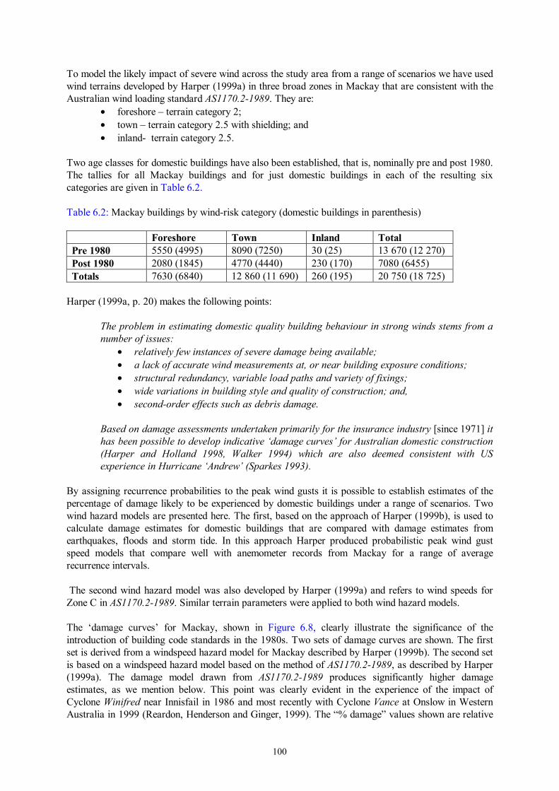
To model the likely impact of severe wind across the study area from a range of scenarios we have used wind terrains developed by Harper (1999a) in three broad zones in Mackay that are consistent with the Australian wind loading standard AS1170.2-1989. They are:

• foreshore – terrain category 2; • town – terrain category 2.5 with shielding; and • inland- terrain category 2.5.

Two age classes for domestic buildings have also been established, that is, nominally pre and post 1980. The tallies for all Mackay buildings and for just domestic buildings in each of the resulting six categories are given in Table 6.2. Table 6.2: Mackay buildings by wind-risk category (domestic buildings in parenthesis) Foreshore Town Inland Total Pre 1980 5550 (4995) 8090 (7250) 30 (25) 13 670 (12 270) Post 1980 2080 (1845) 4770 (4440) 230 (170) 7080 (6455) Totals 7630 (6840) 12 860 (11 690) 260 (195) 20 750 (18 725)

Harper (1999a, p. 20) makes the following points:

The problem in estimating domestic quality building behaviour in strong winds stems from a number of issues:

• relatively few instances of severe damage being available; • a lack of accurate wind measurements at, or near building exposure conditions; • structural redundancy, variable load paths and variety of fixings; • wide variations in building style and quality of construction; and, • second-order effects such as debris damage.

Based on damage assessments undertaken primarily for the insurance industry [since 1971] it has been possible to develop indicative ‘damage curves’ for Australian domestic construction (Harper and Holland 1998, Walker 1994) which are also deemed consistent with US experience in Hurricane ‘Andrew’ (Sparkes 1993).

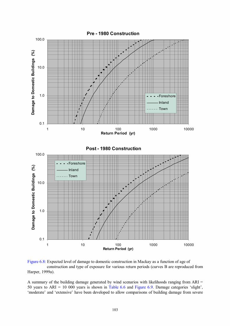
By assigning recurrence probabilities to the peak wind gusts it is possible to establish estimates of the percentage of damage likely to be experienced by domestic buildings under a range of scenarios. Two wind hazard models are presented here. The first, based on the approach of Harper (1999b), is used to calculate damage estimates for domestic buildings that are compared with damage estimates from earthquakes, floods and storm tide. In this approach Harper produced probabilistic peak wind gust speed models that compare well with anemometer records from Mackay for a range of average recurrence intervals. The second wind hazard model was also developed by Harper (1999a) and refers to wind speeds for Zone C in AS1170.2-1989. Similar terrain parameters were applied to both wind hazard models. The ‘damage curves’ for Mackay, shown in Figure 6.8, clearly illustrate the significance of the introduction of building code standards in the 1980s. Two sets of damage curves are shown. The first set is derived from a windspeed hazard model for Mackay described by Harper (1999b). The second set is based on a windspeed hazard model based on the method of AS1170.2-1989, as described by Harper (1999a). The damage model drawn from AS1170.2-1989 produces significantly higher damage estimates, as we mention below. This point was clearly evident in the experience of the impact of Cyclone Winifred near Innisfail in 1986 and most recently with Cyclone Vance at Onslow in Western Australia in 1999 (Reardon, Henderson and Ginger, 1999). The “% damage” values shown are relative

101

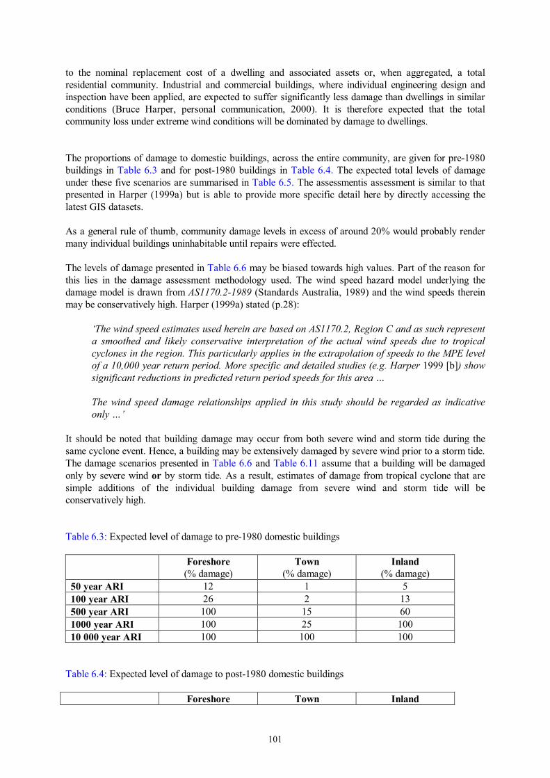
to the nominal replacement cost of a dwelling and associated assets or, when aggregated, a total residential community. Industrial and commercial buildings, where individual engineering design and inspection have been applied, are expected to suffer significantly less damage than dwellings in similar conditions (Bruce Harper, personal communication, 2000). It is therefore expected that the total community loss under extreme wind conditions will be dominated by damage to dwellings. The proportions of damage to domestic buildings, across the entire community, are given for pre-1980 buildings in Table 6.3 and for post-1980 buildings in Table 6.4. The expected total levels of damage under these five scenarios are summarised in Table 6.5. The assessmentis assessment is similar to that presented in Harper (1999a) but is able to provide more specific detail here by directly accessing the latest GIS datasets. As a general rule of thumb, community damage levels in excess of around 20% would probably render many individual buildings uninhabitable until repairs were effected. The levels of damage presented in Table 6.6 may be biased towards high values. Part of the reason for this lies in the damage assessment methodology used. The wind speed hazard model underlying the damage model is drawn from AS1170.2-1989 (Standards Australia, 1989) and the wind speeds therein may be conservatively high. Harper (1999a) stated (p.28):

‘The wind speed estimates used herein are based on AS1170.2, Region C and as such represent a smoothed and likely conservative interpretation of the actual wind speeds due to tropical cyclones in the region. This particularly applies in the extrapolation of speeds to the MPE level of a 10,000 year return period. More specific and detailed studies (e.g. Harper 1999 [b]) show significant reductions in predicted return period speeds for this area … The wind speed damage relationships applied in this study should be regarded as indicative only …’

It should be noted that building damage may occur from both severe wind and storm tide during the same cyclone event. Hence, a building may be extensively damaged by severe wind prior to a storm tide. The damage scenarios presented in Table 6.6 and Table 6.11 assume that a building will be damaged only by severe wind or by storm tide. As a result, estimates of damage from tropical cyclone that are simple additions of the individual building damage from severe wind and storm tide will be conservatively high. Table 6.3: Expected level of damage to pre-1980 domestic buildings

Foreshore (% damage)

Town (% damage)

Inland (% damage)

50 year ARI 12 1 5 100 year ARI 26 2 13 500 year ARI 100 15 60 1000 year ARI 100 25 100 10 000 year ARI 100 100 100

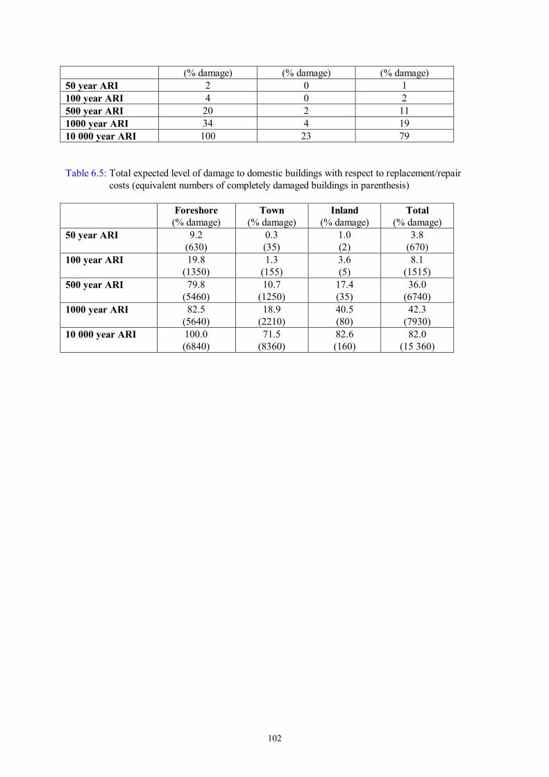
Table 6.4: Expected level of damage to post-1980 domestic buildings

Foreshore Town Inland

102

(% damage) (% damage) (% damage) 50 year ARI 2 0 1 100 year ARI 4 0 2 500 year ARI 20 2 11 1000 year ARI 34 4 19 10 000 year ARI 100 23 79 Table 6.5: Total expected level of damage to domestic buildings with respect to replacement/repair

costs (equivalent numbers of completely damaged buildings in parenthesis)

Foreshore (% damage)

Town (% damage)

Inland (% damage)

Total (% damage)

50 year ARI 9.2 (630)

0.3 (35)

1.0 (2)

3.8 (670)

100 year ARI 19.8 (1350)

1.3 (155)

3.6 (5)

8.1 (1515)

500 year ARI 79.8 (5460)

10.7 (1250)

17.4 (35)

36.0 (6740)

1000 year ARI 82.5 (5640)

18.9 (2210)

40.5 (80)

42.3 (7930)

10 000 year ARI 100.0 (6840)

71.5 (8360)

82.6 (160)

82.0 (15 360)

103

Pre - 1980 Construction

0.1

1.0

10.0

100.0

1 10 100 1000 10000Return Period (yr)

Dam

age

to D

omes

tic B

uild

ings

(%

)

Foreshore

Inland

Town

Post - 1980 Construction

0.1

1.0

10.0

100.0

1 10 100 1000 10000Return Period (yr)

Dam

age

to D

omes

tic B

uild

ings

(%

) Foreshore

Inland

Town

Figure 6.8: Expected level of damage to domestic construction in Mackay as a function of age of

construction and type of exposure for various return periods (curves B are reproduced from Harper, 1999a).

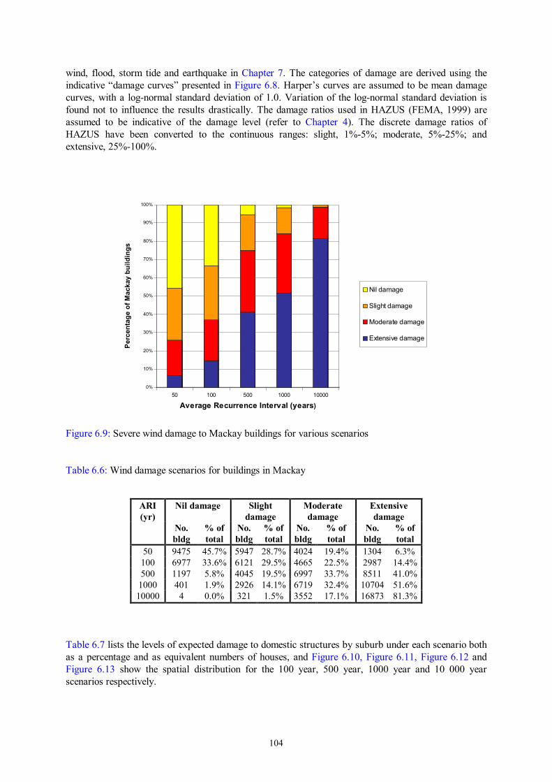
A summary of the building damage generated by wind scenarios with likelihoods ranging from ARI = 50 years to ARI = 10 000 years is shown in Table 6.6 and Figure 6.9. Damage categories ‘slight’, ‘moderate’ and ‘extensive’ have been developed to allow comparisons of building damage from severe

104

wind, flood, storm tide and earthquake in Chapter 7. The categories of damage are derived using the indicative “damage curves” presented in Figure 6.8. Harper’s curves are assumed to be mean damage curves, with a log-normal standard deviation of 1.0. Variation of the log-normal standard deviation is found not to influence the results drastically. The damage ratios used in HAZUS (FEMA, 1999) are assumed to be indicative of the damage level (refer to Chapter 4). The discrete damage ratios of HAZUS have been converted to the continuous ranges: slight, 1%-5%; moderate, 5%-25%; and extensive, 25%-100%.

Figure 6.9: Severe wind damage to Mackay buildings for various scenarios Table 6.6: Wind damage scenarios for buildings in Mackay

ARI (yr)

Nil damage Slight damage

Moderate damage

Extensive damage

No. bldg

% of total

No. bldg

% of total

No. bldg

% of total

No. bldg

% of total

50 9475 45.7% 5947 28.7% 4024 19.4% 1304 6.3% 100 6977 33.6% 6121 29.5% 4665 22.5% 2987 14.4% 500 1197 5.8% 4045 19.5% 6997 33.7% 8511 41.0%

1000 401 1.9% 2926 14.1% 6719 32.4% 10704 51.6% 10000 4 0.0% 321 1.5% 3552 17.1% 16873 81.3%

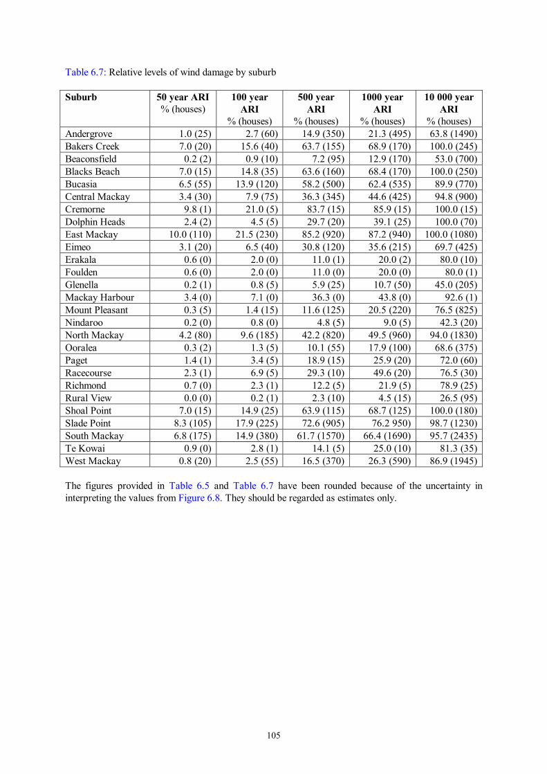
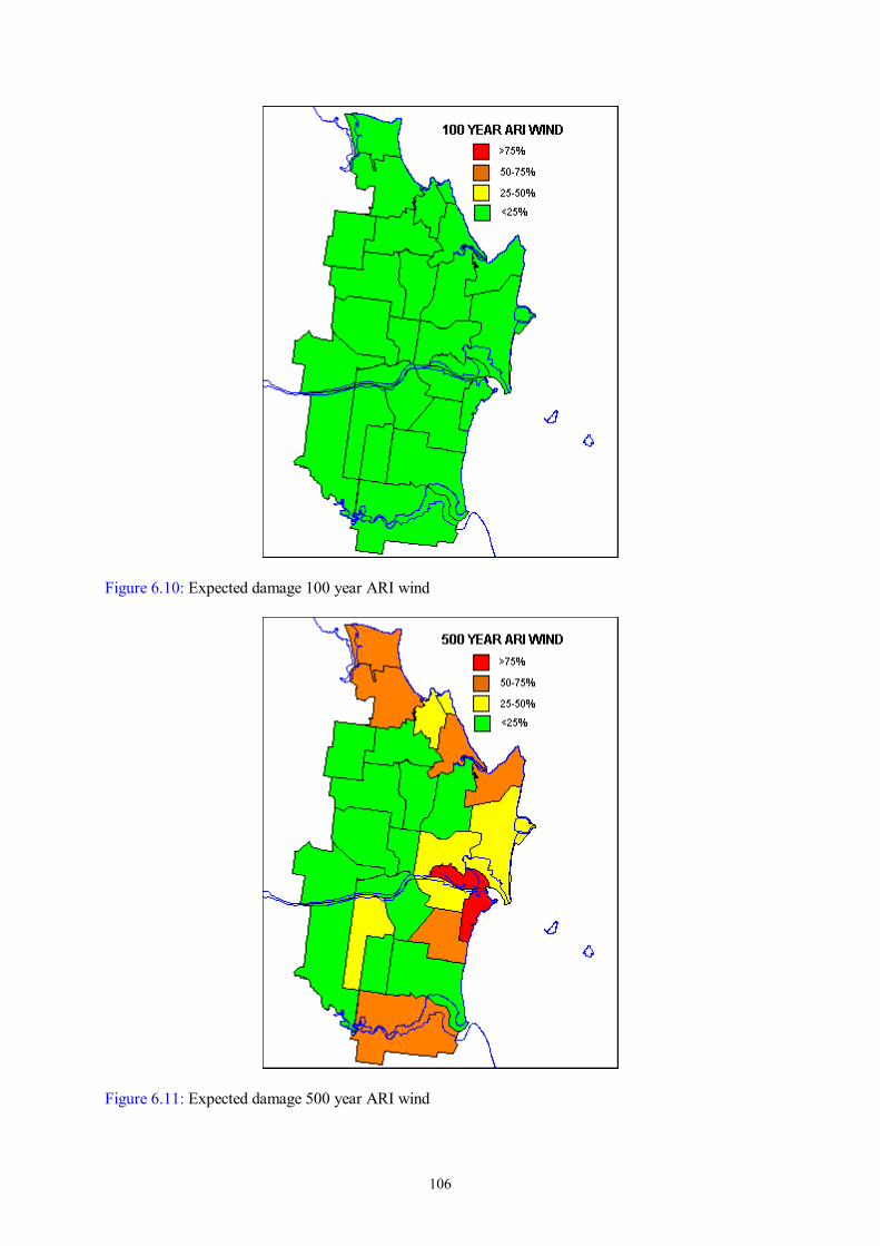
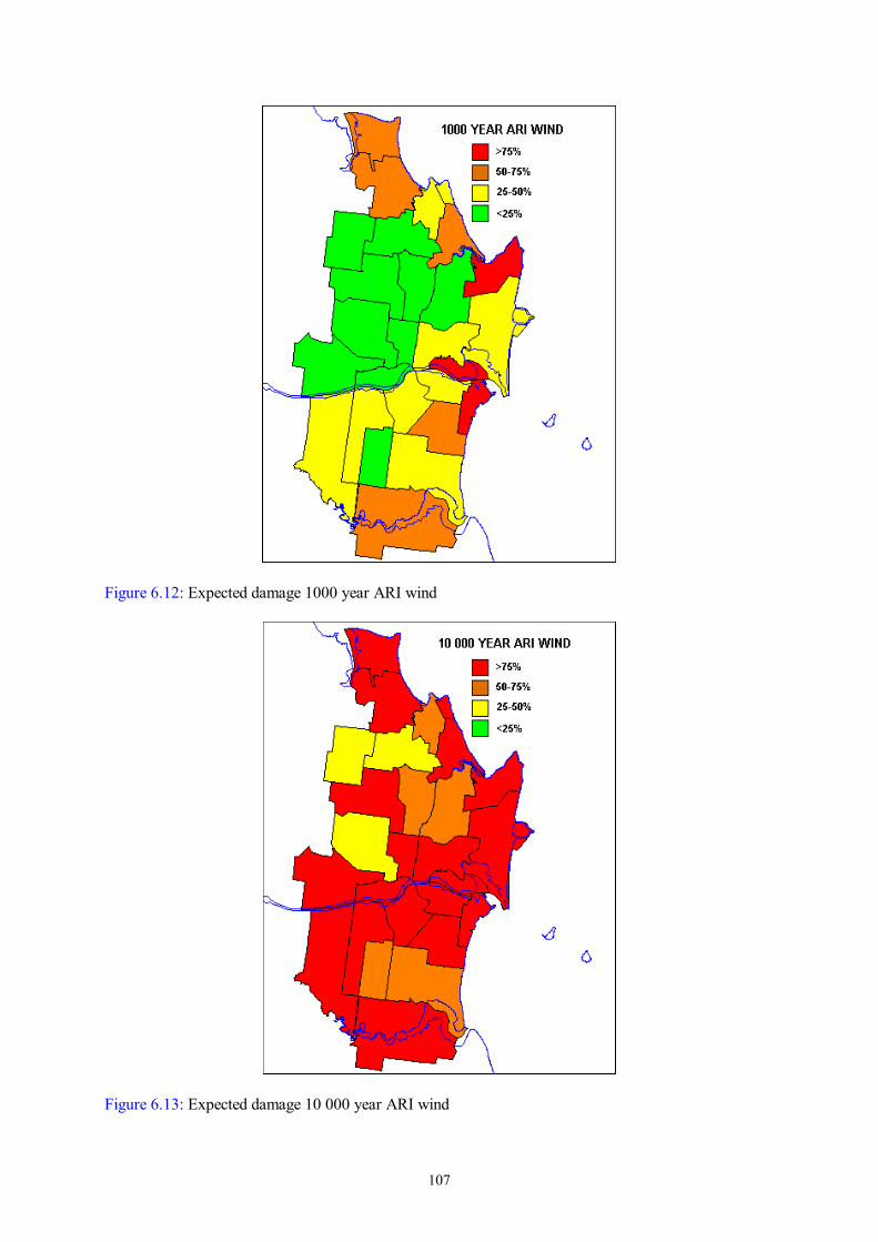
Table 6.7 lists the levels of expected damage to domestic structures by suburb under each scenario both as a percentage and as equivalent numbers of houses, and Figure 6.10, Figure 6.11, Figure 6.12 and Figure 6.13 show the spatial distribution for the 100 year, 500 year, 1000 year and 10 000 year scenarios respectively.

50 100 500 1000 100000%

10%

20%

30%

40%

50%

60%

70%

80%

90%

100%

Perc

enta

ge o

f Mac

kay

build

ings

Average Recurrence Interval (years)

Nil damage

Slight damage

Moderate damage

Extensive damage

105

Table 6.7: Relative levels of wind damage by suburb Suburb 50 year ARI

% (houses) 100 year

ARI % (houses)

500 year ARI

% (houses)

1000 year ARI

% (houses)

10 000 year ARI

% (houses) Andergrove 1.0 (25) 2.7 (60) 14.9 (350) 21.3 (495) 63.8 (1490)Bakers Creek 7.0 (20) 15.6 (40) 63.7 (155) 68.9 (170) 100.0 (245)Beaconsfield 0.2 (2) 0.9 (10) 7.2 (95) 12.9 (170) 53.0 (700)Blacks Beach 7.0 (15) 14.8 (35) 63.6 (160) 68.4 (170) 100.0 (250)Bucasia 6.5 (55) 13.9 (120) 58.2 (500) 62.4 (535) 89.9 (770)Central Mackay 3.4 (30) 7.9 (75) 36.3 (345) 44.6 (425) 94.8 (900)Cremorne 9.8 (1) 21.0 (5) 83.7 (15) 85.9 (15) 100.0 (15)Dolphin Heads 2.4 (2) 4.5 (5) 29.7 (20) 39.1 (25) 100.0 (70)East Mackay 10.0 (110) 21.5 (230) 85.2 (920) 87.2 (940) 100.0 (1080)Eimeo 3.1 (20) 6.5 (40) 30.8 (120) 35.6 (215) 69.7 (425)Erakala 0.6 (0) 2.0 (0) 11.0 (1) 20.0 (2) 80.0 (10)Foulden 0.6 (0) 2.0 (0) 11.0 (0) 20.0 (0) 80.0 (1)Glenella 0.2 (1) 0.8 (5) 5.9 (25) 10.7 (50) 45.0 (205)Mackay Harbour 3.4 (0) 7.1 (0) 36.3 (0) 43.8 (0) 92.6 (1)Mount Pleasant 0.3 (5) 1.4 (15) 11.6 (125) 20.5 (220) 76.5 (825)Nindaroo 0.2 (0) 0.8 (0) 4.8 (5) 9.0 (5) 42.3 (20)North Mackay 4.2 (80) 9.6 (185) 42.2 (820) 49.5 (960) 94.0 (1830)Ooralea 0.3 (2) 1.3 (5) 10.1 (55) 17.9 (100) 68.6 (375)Paget 1.4 (1) 3.4 (5) 18.9 (15) 25.9 (20) 72.0 (60)Racecourse 2.3 (1) 6.9 (5) 29.3 (10) 49.6 (20) 76.5 (30)Richmond 0.7 (0) 2.3 (1) 12.2 (5) 21.9 (5) 78.9 (25)Rural View 0.0 (0) 0.2 (1) 2.3 (10) 4.5 (15) 26.5 (95)Shoal Point 7.0 (15) 14.9 (25) 63.9 (115) 68.7 (125) 100.0 (180)Slade Point 8.3 (105) 17.9 (225) 72.6 (905) 76.2 950) 98.7 (1230)South Mackay 6.8 (175) 14.9 (380) 61.7 (1570) 66.4 (1690) 95.7 (2435)Te Kowai 0.9 (0) 2.8 (1) 14.1 (5) 25.0 (10) 81.3 (35)West Mackay 0.8 (20) 2.5 (55) 16.5 (370) 26.3 (590) 86.9 (1945) The figures provided in Table 6.5 and Table 6.7 have been rounded because of the uncertainty in interpreting the values from Figure 6.8. They should be regarded as estimates only.

106

Figure 6.10: Expected damage 100 year ARI wind

Figure 6.11: Expected damage 500 year ARI wind

107

Figure 6.12: Expected damage 1000 year ARI wind

Figure 6.13: Expected damage 10 000 year ARI wind

108

Lifelines and other assets: With most cyclones that approach to within the radius of maximum winds, the greatest amount of inconvenience has been caused by damage to the power reticulation infrastructure. Power lines are often brought down by tree branches, palm fronds and other wind-blown debris. Electricity authorities in coastal areas of Queensland tend to maintain good clearance of trees from power lines and the more critical areas tend to be serviced by underground mains. Whilst it is unusual for power poles and pylons to be brought down by high winds, it certainly has happened. In the Brisbane Valley in 1999, for example, several transmission line pylons were brought down in extreme wind gusts associated with a local storm (in the type of micro-burst conditions that could be experienced in the tornadic outbreaks experienced in cyclones). Also in Cyclone Steve in Cairns (late February 2000), several poles were pushed out of the vertical because the ground they were in had been saturated by up to four weeks of continual heavy rainfall before the severe winds were experienced. Tree-fall also represents a significant threat to buildings, life and assets such as cars. Trees will also block roads and may even dislocate underground utilities, such as water mains, if their root systems are extensive. Again, saturation of the soil ahead of severe wind will increase the likelihood of trees being brought down. The disposal of debris produced by wind damage to trees in cyclones inevitably presents the Council’s waste managers with a major challenge. Strong winds also pose a threat to telecommunications, especially those which utilise above ground infrastructure such as microwave dishes, aerials, radio transponders and satellite dishes. This infrastructure is particularly susceptible because most of it relies on line-of-sight operation. The misalignment of antennae by the wind will disrupt the networks that they support. In stronger winds, the large transmission or relay towers may even be brought down. The substantial commercial and pleasure boat fleets in Mackay are also at risk in strong winds and waves. During Cyclone Kerry in 1971, for example, many pleasure craft and small boats were damaged or destroyed inside the protection of the outer harbour. During cyclone alerts, many small craft take shelter in, or close to the mangroves that fringe Bassett Basin, though the recent completion of a major marina immediately south of the outer harbour may provide greater protection for such craft. Strong winds also carry salt spray from the surf many kilometres inland. This has a short-term impact on vegetation through scalding, but will also have a longer-term impact on ferrous metal in buildings, cars, and so on, unless it is washed away by fresh water fairly quickly.

Storm Tide Risks In terms of loss of life, the impact of the 1918 Mackay storm tide, where at least 13 people drowned, ranks behind Cyclone Mahina (where close to 400 pearling fleet crew drowned in Bathurst Bay in 1899), and the March 1918 Innisfail cyclone (where as many as 100 died). The 1918 Mackay storm tide is, however, the most destructive storm tide event to have impacted an urban area in Australia. A storm tide is created by the combined action of the storm surge produced by the cyclone, and the normal sea level produced by the astronomical tide. Storm surges are generated by a combination of the inverted barometer effect and wind stress. The actual height of the surge at the coastline is strongly influenced by these characteristics including the angle at which the cyclone crosses the coast. The influence of each is affected by conditions near the site where the cyclone makes landfall, including coastal geometry and tides. Each of these influences will be considered below. The lowering of atmospheric pressure is the factor that has the greatest influence on surge height in the open sea. This so-called “inverse barometer” effect generates a hydrostatic rise of sea level of approximately 1 cm for each hectopascal (hPa) drop in pressure. During the most severe storms, a

109

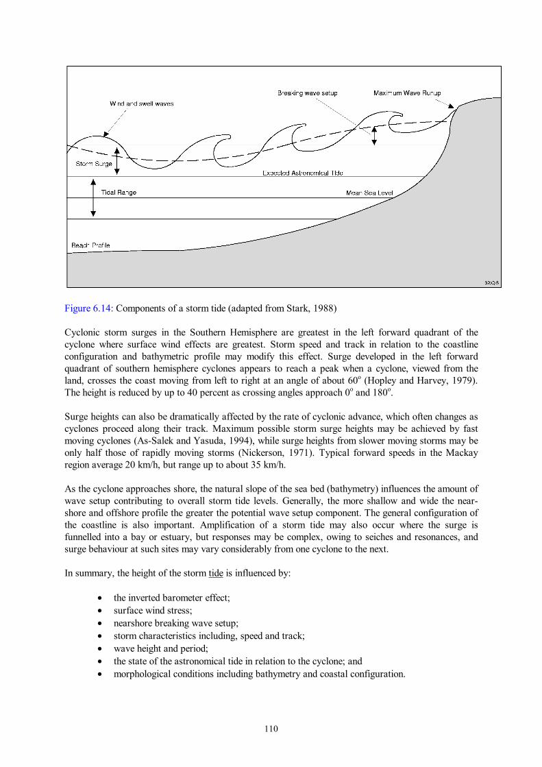
pressure drop of up to 100 hPa is possible; hence, it is unlikely that the inverse barometer effect could produce an open water sea level rise much greater than 1 m. In deep water this is the only factor contributing to changes in still-water levels (Simpson and Riehl, 1981). The other factor directly responsible for a storm surge is severe wind stress applied to the ocean surface that results in a gradual acceleration of the near-surface layer. In deep water there is no net significant wind-driven transport of water because countercurrents established at depth compensate for the surface transport. As the wind-driven surface flow enters shallow water, however, seabed friction retards the counter currents, leading to an increase in water level (setup) which reaches a maximum at the shoreline. Wind-driven surface flow can also cause a depression of the water surface when winds blow offshore leading to a decrease in the water level (setdown). The storm surge is thus caused by the combined influence of the inverted barometer effect along with wind-driven currents that are controlled by wind velocities and the fetch or distance over which the wind blows. The intense circulating surface winds of tropical cyclones also generate short period surface waves (sea and swell) which propagate out from the storm centre. These waves ride upon the elevated long period storm surge and may attack beaches and coastal margins at higher than normal elevations. Nearshore breaking wave setup also adds to the overall quantum of sea level increase produced in a storm tide. Wave setup is defined as the super-elevation of the mean water level caused by wave action alone, and occurs largely in the inshore zone where waves break and impart a shoreward flux of momentum (Komar, 1976). Where the water depth shoals rapidly towards the shoreline, wave setup may constitute a significant proportion of the total surge (Simpson and Riehl, 1981). It follows that for islands in deep water the wave setup component may exceed both the wind stress and inverted barometer surge components. As a wave moves shoreward on a sloping bottom, the process of shoaling causes the amplitude to increase until the wave breaks when the ratio of wave height to still water depth is about 0.78. Wave setup occurs because breaking waves transport water shorewards, causing the water surface to rise from the breaker zone to the shoreline. It follows then, that larger waves transport more water shoreward when they break and produce a larger setup. Simpson and Riehl (1981), studying the storm surge associated with Cyclone Eloise (1975), deduced that wave setup contributed 1.4 m to the surge height, which reached 4.9 m above still water level. Overall storm tide height is therefore, determined by the combination of the storm surge, wave setup and height of the astronomical tide at the time the cyclone crosses the coast. In general, areas with a high tidal range have a lower probability of extensive surge flooding than areas with a small tidal range, because tidal channels and intertidal flats are extensively exposed and the mean water level is substantially below low-lying land areas for most of the tidal cycle. It has become standard practice for emergency managers to relate storm tide inundation levels to the Highest Astronomical Tide (HAT). In Mackay, HAT is approximately 3.66 m above mean sea level (or AHD), whilst lowest astronomical tide (LAT) is 3.04 m below AHD. A storm surge of 3 m, therefore, would be entirely absorbed by the tidal range were it to arrive at half tide or less, but would inundate land up to 3 m above the highest tide level if it coincided with the HAT. It is probable that storm tide inundation would tend to last for six hours or less. The various elements of the storm tide are illustrated in Figure 6.14.

110

Figure 6.14: Components of a storm tide (adapted from Stark, 1988) Cyclonic storm surges in the Southern Hemisphere are greatest in the left forward quadrant of the cyclone where surface wind effects are greatest. Storm speed and track in relation to the coastline configuration and bathymetric profile may modify this effect. Surge developed in the left forward quadrant of southern hemisphere cyclones appears to reach a peak when a cyclone, viewed from the land, crosses the coast moving from left to right at an angle of about 60o (Hopley and Harvey, 1979). The height is reduced by up to 40 percent as crossing angles approach 0o and 180o. Surge heights can also be dramatically affected by the rate of cyclonic advance, which often changes as cyclones proceed along their track. Maximum possible storm surge heights may be achieved by fast moving cyclones (As-Salek and Yasuda, 1994), while surge heights from slower moving storms may be only half those of rapidly moving storms (Nickerson, 1971). Typical forward speeds in the Mackay region average 20 km/h, but range up to about 35 km/h. As the cyclone approaches shore, the natural slope of the sea bed (bathymetry) influences the amount of wave setup contributing to overall storm tide levels. Generally, the more shallow and wide the near-shore and offshore profile the greater the potential wave setup component. The general configuration of the coastline is also important. Amplification of a storm tide may also occur where the surge is funnelled into a bay or estuary, but responses may be complex, owing to seiches and resonances, and surge behaviour at such sites may vary considerably from one cyclone to the next. In summary, the height of the storm tide is influenced by:

• the inverted barometer effect; • surface wind stress; • nearshore breaking wave setup; • storm characteristics including, speed and track; • wave height and period; • the state of the astronomical tide in relation to the cyclone; and • morphological conditions including bathymetry and coastal configuration.

111

The threat posed by the storm tide is then the sum of these influences in relation to the community at risk. The location of crossing is important given that the maximum surge height on the Queensland coast will be to the left of the storm’s track near the forward left quadrant of the cyclone in the band of maximum onshore winds (i.e. close to the eye wall). A cyclone crossing the coast 25 to 50 km to the north of Mackay, therefore, will produce a greater storm tide than a cyclone crossing directly over, or to the south of the city. Areas to the north of the crossing point may experience reduced surge levels or even setdown. Inundation by storm tide can last up to around six to eight hours and largely subsides with the next low tide. The outward run of this water, combined with flooding from intense cyclonic rainfall not only raises the level of the storm surge but also presents a hazard as it has its own velocity seaward which can increase as the storm tide recedes. This ‘back wash’ is often associated with scouring around structures and the mobilisation of large volumes of debris.

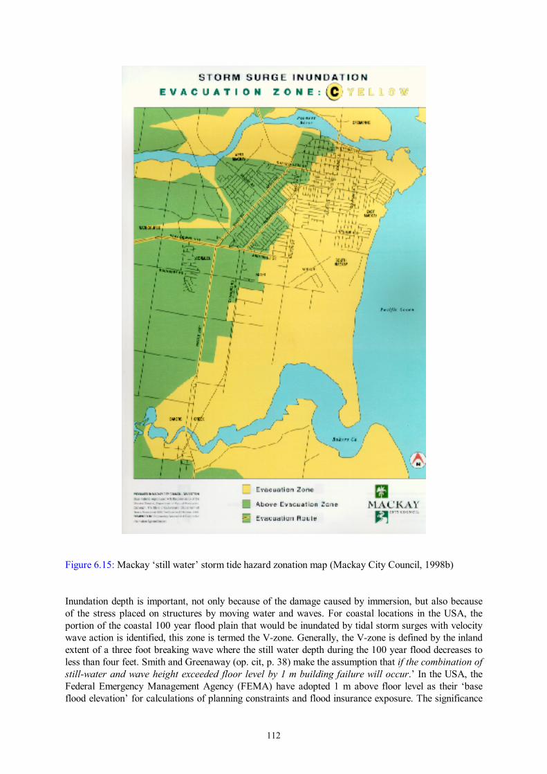
Vulnerability to Storm Tide Most models and hazard maps of storm tide adopt a ‘still water’ inundation approach that simply delimits the area affected by the horizontal contour equivalent to the storm tide elevation. Figure 6.15 is an example of a ‘still water’ storm tide hazard map of Mackay. It has been taken from the Action Guide produced by Mackay City Council (1998b) to educate the community on a range of risks, including storm tide. It shows the area that would be inundated by a storm tide 4 m above HAT, and shows therefore, the area that would need to be evacuated in advance of a storm tide. It was developed by simply taking the contour that represents the level that is 4 m above HAT. ‘Still water’ mapping, similar to this example, but employing up to five zones in increments of one metre above HAT, is now the Queensland standard. The ‘still water’ model does not take account of any wave setup or wave runup (the height to which the momentum of broken waves can carry them up the shore face). Sea wave height and power, however, decay rapidly as the surge moves inland. Smith and Greenaway (1994, Figure 3.7), for example, provide a curve representing ‘velocity decay’, relative to distance from the shoreline, for Mackay. This curve was based on the North American experience of storm tide and shows that the velocity of sea waves, based on a wind speed of 130 km/h, declines from 1.54 m/sec to 0.5 m/sec within 500 m of the shore. Whilst the destructive potential of sea waves declines rapidly inland, shallow water, wind-driven waves may be present in some areas inundated by the storm tide. With the inshore propagation of the storm surge, wind waves can propagate substantially further inland than would normally occur, producing unusual erosion or deposition. Jelenianski (1989, in Chowdhury, 1994), calculated that the height of wind waves in shallow waters (crest to trough) could be as much as 50% to 75% of the depth of over-land inundation. For convenience of model computation we adopted an overall average of 60%. The addition to total water level by these waves would, therefore, be half of that value, i.e. 30%.

112

Figure 6.15: Mackay ‘still water’ storm tide hazard zonation map (Mackay City Council, 1998b) Inundation depth is important, not only because of the damage caused by immersion, but also because of the stress placed on structures by moving water and waves. For coastal locations in the USA, the portion of the coastal 100 year flood plain that would be inundated by tidal storm surges with velocity wave action is identified, this zone is termed the V-zone. Generally, the V-zone is defined by the inland extent of a three foot breaking wave where the still water depth during the 100 year flood decreases to less than four feet. Smith and Greenaway (op. cit, p. 38) make the assumption that if the combination of still-water and wave height exceeded floor level by 1 m building failure will occur.’ In the USA, the Federal Emergency Management Agency (FEMA) have adopted 1 m above floor level as their ‘base flood elevation’ for calculations of planning constraints and flood insurance exposure. The significance

113

of this elevation was demonstrated in coastal areas that experienced the impact of Hurricane Hugo in 1989. FEMA (1992), quoted by Smith and Greenaway (ibid), state that:

Practically all residential structures not elevated above the base flood level sustained major damage or complete destruction, from either collapse under wave force, floating off foundations, or water washing through and demolishing the structures… as long as adequate openings were left under the living space, Hugo’s surge and waves passed beneath [properly elevated] structures.

It is important to note that no concession is made regarding the form of construction. It is likely, however, that structures engineered to withstand the high levels of lateral loads typical of those established in the wind or earthquake components of the Australian Design Loading Standards, would perform better than those built to lesser levels of strength. One would expect light timber-framed buildings with fibro cladding to be less resilient than reinforced concrete block buildings, for example. The experience in the USA indicates that substantial engineered buildings are not immune to total destruction from storm tide, especially if they are located along the foreshore ‘front row’ where sea wave power and height are at their greatest. The literature is not clear, however, as to the degree of risk associated with inundation of water of more than 1 m over floor level at a distance from the shoreline where water velocity is relatively minimal, i.e. more than say 1.5 km from the shore, as could be the case in large parts of Mackay. The scouring associated with the retreating water at the next low tide may further attack structures weakened by the initial impact of the storm tide. Scouring may also damage roads, bridge approaches and underground utilities, such as water mains, in some areas. People who remain in areas subject to storm tide inundation are at substantial risk of drowning, especially if they are out of doors and in buildings prone to failure. Even where people are inside their houses or other shelter, the risk of drowning increases with the height of water over floor level. Clearly, those people sheltering in buildings that are likely to have more than 1 m over floor level should be evacuated well before the cyclone crosses the coast. In addition to the loss caused by the severe damage to, or demolition of buildings, the damage done to building contents would be substantial. Smith and Greenaway (ibid) assume a total loss of contents, such as floor coverings, built-in cupboards, white goods and commercial stock, where inundation is over floor level. They do not, however, estimate damage to assets, such as vehicles or mechanical equipment exposed at ground level. The life of electrical or electronic facilities, such as electric motors or underground telecommunications infrastructure, will be significantly reduced, if not terminated, should they be exposed to inundation. Given that seawater is involved, corrosion is probably a greater problem than with fresh (muddy) water associated river flooding. Salt scalding is also likely to cause the loss of plants, including sugar cane. There is little evidence in the literature, however, of storm tide inundation causing long-term harm to agricultural production as a result of soil salination, probably because the salt is typically flushed away by heavy rain or river flooding following cyclone impact.

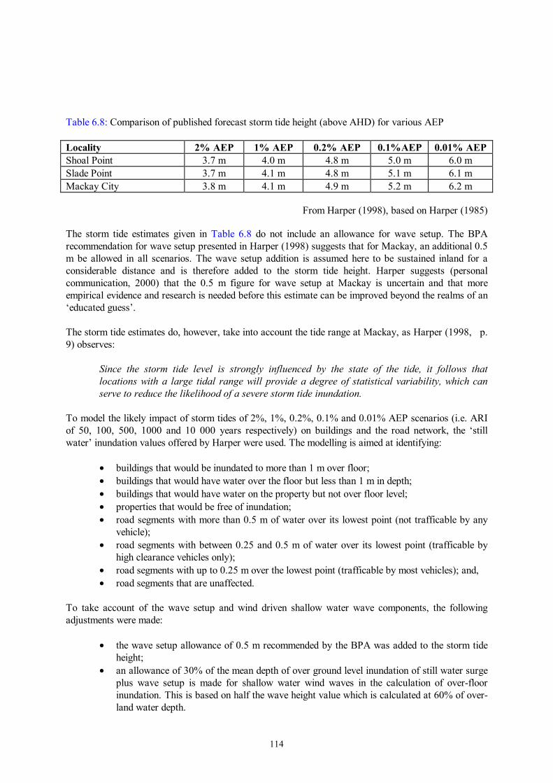
Storm Tide Risk Scenarios The storm tide height (above AHD) annual exceedence probabilities (AEP) cited in Appendix 2 in Harper (1998), which are based on published estimates by the same author in 1985, are given in Table 6.8. The difference between the northern beach suburbs and the city area are explained in terms of off-shore bathymetry.

114

Table 6.8: Comparison of published forecast storm tide height (above AHD) for various AEP Locality 2% AEP 1% AEP 0.2% AEP 0.1%AEP 0.01% AEP Shoal Point 3.7 m 4.0 m 4.8 m 5.0 m 6.0 m Slade Point 3.7 m 4.1 m 4.8 m 5.1 m 6.1 m Mackay City 3.8 m 4.1 m 4.9 m 5.2 m 6.2 m

From Harper (1998), based on Harper (1985)

The storm tide estimates given in Table 6.8 do not include an allowance for wave setup. The BPA recommendation for wave setup presented in Harper (1998) suggests that for Mackay, an additional 0.5 m be allowed in all scenarios. The wave setup addition is assumed here to be sustained inland for a considerable distance and is therefore added to the storm tide height. Harper suggests (personal communication, 2000) that the 0.5 m figure for wave setup at Mackay is uncertain and that more empirical evidence and research is needed before this estimate can be improved beyond the realms of an ‘educated guess’. The storm tide estimates do, however, take into account the tide range at Mackay, as Harper (1998, p. 9) observes:

Since the storm tide level is strongly influenced by the state of the tide, it follows that locations with a large tidal range will provide a degree of statistical variability, which can serve to reduce the likelihood of a severe storm tide inundation.

To model the likely impact of storm tides of 2%, 1%, 0.2%, 0.1% and 0.01% AEP scenarios (i.e. ARI of 50, 100, 500, 1000 and 10 000 years respectively) on buildings and the road network, the ‘still water’ inundation values offered by Harper were used. The modelling is aimed at identifying:

• buildings that would be inundated to more than 1 m over floor; • buildings that would have water over the floor but less than 1 m in depth; • buildings that would have water on the property but not over floor level; • properties that would be free of inundation; • road segments with more than 0.5 m of water over its lowest point (not trafficable by any

vehicle); • road segments with between 0.25 and 0.5 m of water over its lowest point (trafficable by

high clearance vehicles only); • road segments with up to 0.25 m over the lowest point (trafficable by most vehicles); and, • road segments that are unaffected.

To take account of the wave setup and wind driven shallow water wave components, the following adjustments were made:

• the wave setup allowance of 0.5 m recommended by the BPA was added to the storm tide height;

• an allowance of 30% of the mean depth of over ground level inundation of still water surge plus wave setup is made for shallow water wind waves in the calculation of over-floor inundation. This is based on half the wave height value which is calculated at 60% of over-land water depth.

115

Buildings that are within 150 m of the shoreline which have over-floor inundation were further identified because of the heightened risk posed by sea wave velocity and a degree of additional inundation from the broken (foam) component of waves that break close to the shore line. Although this distance is arbitrary, the authors consider it to be a reasonable estimate and a pertinent issue. At present, published model results do not indicate the movement of surge onshore or the lateral translation of that surge. In light of the uncertainties surrounding these aspects of surge it has not been possible to apply any spatial constraints in this study. As such, the analysis produces a generic ‘worst case’ assessment of storm tide exposure across the area of study. This potential over estimation of the spatial extent must be taken into account when interpreting cyclonic surge risk. It is hoped it may be more clearly defined with the application of more advanced modelling capabilities. This conservative approach is consistent with the stated needs of emergency managers. The resulting figures should be seen as reflecting the upper level of impact estimates. Data uncertainty: In this model, the key values of floor height and ground height were taken from the detailed building database described in Chapter 3 and Appendix B. Floor heights were estimated in the field for most buildings and are, for at least 90% of buildings observed in the field, accurate to within 0.25 m. Where buildings were not observed in the field by us, but were surveyed by Smith in 1993, floor heights were generalised into three categories – on slab (0.3 m), suspended floor (0.5 m) and high set (2.0 m). The values collected by Smith are only marginally less accurate than those collected by the Cities Project. Where buildings were not surveyed, a default value of 0.3 m (i.e. slab-on-ground construction), was used. The ground height for each building and road segment was interpolated in the geographical information system (GIS) from the digital elevation model (DEM) developed by Andre Zerger. Given the large scale topographic mapping and photogrammetric sources used for this elevation model, inherent uncertainties exist for the interpolated elevation data. Zerger (1998) reports that 90% of the elevation values in the DEM are accurate to at least 0.3 m. The use of such ‘imprecise’ data may seem to introduce potentially significant error or uncertainty in the outcome. It should be recognised, however, that the error estimates for the DEM produced by Zerger are substantially less than those published for the original topographic data and are the very best available. Few other areas in Australia of elsewhere have contour data of this quality. There are also uncertainties associated with the inundation models used. For example, the uniform 0.5 m wave setup value recommended by the BPA, is sensitive to wave energy which is influenced by cyclone characteristics such as track, velocity and so on. These uncertainties relate to absolute accuracy. In our application of these data, however, we are more interested in relative accuracy, which appears to be quite consistent across regions with similar topography. Given all of the other uncertainties in the model (e.g. with surge height estimates), and the degree of generalisation involved in the analytical process, the uncertainties in elevation (and other input items), probably make little overall difference to the final assessment. Certainly the results reported here are conservative but appear to be both realistic and logical. The storm tide risk model: The buildings subject to inundation at various depths under the five scenarios were identified using the following models for:

• inundation over ground level only: Gd_ht <std + wsu + sww; • inundation over floor level: Fl_ht + Gd_ht <std + wsu + sww; and, • inundation > 1.0 m over floor level: Fl_ht + 1 + Gd_ht <std + wsu + sww.

116

where:

Gd_ht is the height of the ground above AHD; std is storm tide height; Fl_ht is the height of the building floor above ground level; wsu is the wave setup value of 0.5 m; and sww is the height allowance for shallow water wind waves calculated as 30% of the mean

depth of over-ground inundation. The extent of storm tide inundation for the various AEP scenarios are presented in Figures 6.16 to 6.25 and in Figure 6.27. For each of these scenarios the following key applies: • buildings that are likely to have more than 1 m of water over floor level are shown in red; • buildings with water over floor level but less than 1 m in depth are shown in yellow; • buildings with water on the surrounding property but not over floor level are shown in green; and, • properties not affected by inundation are shown in grey. A similar process was used for the road network. No allowance has been made for the frictional effect on the storm tide of buildings, vegetation and micro-relief; nor has the channelling effect of the roads that are perpendicular to the shore been taken into account. The modelling results are summarised in the following discussions of each of the five scenarios. A comparison of the outcomes for the five scenarios is also provided to illustrate the incremental growth of risk as the probability decreases. Assumptions: In the following scenarios two key assumptions have been made. First, that there will be no significant land-based flooding prior to the storm tide impact. We feel that this is a reasonable assumption given that significant storm surges are more likely to be associated with cyclones that move rapidly over the ocean and approach the coast at close to right angles. Such cyclones are less likely than slow moving cyclones to be preceded by substantial rainfall. This assumption appears to be reasonable based on historic experience. For example, the flood which was associated with the 1918 cyclone peaked two days after the passage of the cyclone and the storm tide impact (Gourlay & Hacker, 1986, pp. 193-4). The second assumption is that the population will be concentrated at their place of residence at the time of impact. We feel that this is also a reasonable assumption, given that there would be 24 and 48 hours warning of the impending cyclone impact and that families would seek shelter together at home wherever possible. This is in contrast to the situation with earthquakes (see Chapter 4), where a range of population distribution scenarios (e.g. day, night, weekend, holiday period, etc.) needs to be considered. The 2% AEP scenario: Under this scenario, inundation to a depth of up to 3.8 m of surge plus 0.5 m of wave setup could occur. Such a situation could be caused by a storm surge of as little as 0.8 m above HAT arriving at close to a high tide. By applying this inundation level our model indicates that some 2580 buildings could be affected as follows (rounded numbers):

• a small number of buildings could have water over floor level to a depth of >1 m; • up to 1580 buildings could have water over floor level to a depth of less than 1 m;

117

• up to 1020 buildings could have water on the property, but not over floor level; • the remaining 18 120, or so, buildings would be free of inundation; • 72.9 km of road would not be trafficable (i.e. more than 0.5 m of water over the pavement); • 21.5 km of road would only be trafficable by high clearance vehicles (0.25 to 0.5 m of water

over the pavement); and, • 13.9 km of road would have less than 0.25 m of water over the pavement and would be

trafficable by most vehicles. Overall, the impact of a 2% AEP (ARI of 50 years) storm tide event would certainly cause significant damage to buildings and short-term dislocation would be significant. Greatest impact will be felt in the low lying areas of East Mackay and South Mackay. These areas are further defined by Juliet Street in the west and Hague Street in the east and along the coastal fringe of Slade Point to the north of Seagull Street and west of Slade Point Road, and on the northern side of Ocean Avenue. In that area as many as 3000 cars could be at risk of salt water damage if not moved to higher ground before the impact of the storm tide. The northwestern end of the airport runway would also be inundated. The modelled impact of the study area is shown in Figure 6.16 and a more detailed view of the city area is shown in Figure 6.17.

Figure 6.16: Modelled impact of a 2% AEP Figure 6.17: Modelled impact of a 2% AEP storm tide scenario storm tide scenario (detail) The 1% AEP scenario: The minimum storm surge required to create a storm tide of 4.1 m above AHD (0.6 m above HAT) would be a little over 1 m, arriving at, or close to a very high tide. By applying our model for a storm tide of 4.1 m above AHD and a 0.5 m wave setup figure, around 3410 buildings could be affected as follows (figures rounded):

• up to 60 buildings and other structures would likely fail having more than 1 m of water over floor level;

• up to 2110 buildings could have water over floor level of less than 1 m;

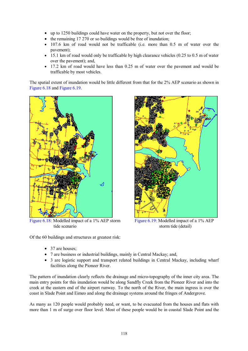
118

• up to 1250 buildings could have water on the property, but not over the floor; • the remaining 17 270 or so buildings would be free of inundation; • 107.6 km of road would not be trafficable (i.e. more than 0.5 m of water over the

pavement); • 15.1 km of road would only be trafficable by high clearance vehicles (0.25 to 0.5 m of water

over the pavement); and, • 17.2 km of road would have less than 0.25 m of water over the pavement and would be

trafficable by most vehicles. The spatial extent of inundation would be little different from that for the 2% AEP scenario as shown in Figure 6.18 and Figure 6.19.

Figure 6.18: Modelled impact of a 1% AEP storm Figure 6.19: Modelled impact of a 1% AEP tide scenario storm tide (detail) Of the 60 buildings and structures at greatest risk:

• 37 are houses; • 7 are business or industrial buildings, mainly in Central Mackay; and, • 3 are logistic support and transport related buildings in Central Mackay, including wharf

facilities along the Pioneer River. The pattern of inundation clearly reflects the drainage and micro-topography of the inner city area. The main entry points for this inundation would be along Sandfly Creek from the Pioneer River and into the creek at the eastern end of the airport runway. To the north of the River, the main ingress is over the coast in Slade Point and Eimeo and along the drainage systems around the fringes of Andergrove. As many as 120 people would probably need, or want, to be evacuated from the houses and flats with more than 1 m of surge over floor level. Most of these people would be in coastal Slade Point and the

119

low-lying fringe areas of Andergrove. It is also likely that a significant number of people in the rest of the storm tide affected areas would evacuate. The impact of a 1% AEP storm tide event would undoubtedly be significant, though fewer than 200 people would probably be at risk of serious harm. Perhaps as many as 60 buildings and other structures could be at risk of destruction or significant damage, with as many as 2100 further buildings likely to suffer substantial contents damage. Some 4100 cars would also be at risk of salt water damage unless they were moved to higher ground in advance of the storm tide impact, and the airport runway would be inundated. The 0.2% AEP scenario: A storm tide inundation level of 4.8 m above AHD (1.3 m above HAT) is essentially identical to that experienced in the 1918 cyclone if allowance for wave setup is also included. By applying our model for a storm tide of 4.8 m above AHD and a 0.5 m wave setup figure, around 5860 buildings and other structures would be affected as follows (numbers rounded):

• as many as 2040 buildings and other structures could have more than 1 m of water over floor level - of these about 175 buildings are within the first 150 m of the shore line, mostly in Eimeo and Slade Point, and along the Pioneer River downstream of the Forgan Bridge. These 175 buildings would have a heightened risk of being destroyed because of sea wave velocities and runup;

• up to 2090 buildings could have water over floor level of less than 1 m depth; • a further 1730 buildings could have water on the property; • the remaining 14 820 or so buildings would be free of inundation; • 162.4 km of road would not be trafficable (i.e. more than 0.5 m of water over the

pavement); • 18.7 km of road would only be trafficable by high clearance vehicles (0.25 to 0.5 m of water

over the pavement); and, • 18.1 km of road would have less than 0.25 m of water over the pavement and would be

trafficable by most vehicles. The spatial distribution of these buildings is shown in Figure 6.20 with closer detail in Figure 6.21.

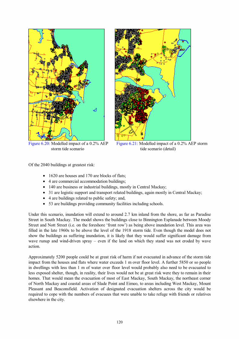
120

Figure 6.20: Modelled impact of a 0.2% AEP Figure 6.21: Modelled impact of a 0.2% AEP storm

storm tide scenario tide scenario (detail) Of the 2040 buildings at greatest risk:

• 1620 are houses and 170 are blocks of flats; • 4 are commercial accommodation buildings; • 140 are business or industrial buildings, mostly in Central Mackay; • 31 are logistic support and transport related buildings, again mostly in Central Mackay; • 4 are buildings related to public safety; and, • 53 are buildings providing community facilities including schools.

Under this scenario, inundation will extend to around 2.7 km inland from the shore, as far as Paradise Street in South Mackay. The model shows the buildings close to Binnington Esplanade between Moody Street and Nott Street (i.e. on the foreshore ‘front row’) as being above inundation level. This area was filled in the late 1960s to be above the level of the 1918 storm tide. Even though the model does not show the buildings as suffering inundation, it is likely that they would suffer significant damage from wave runup and wind-driven spray – even if the land on which they stand was not eroded by wave action. Approximately 5200 people could be at great risk of harm if not evacuated in advance of the storm tide impact from the houses and flats where water exceeds 1 m over floor level. A further 5850 or so people in dwellings with less than 1 m of water over floor level would probably also need to be evacuated to less exposed shelter, though, in reality, their lives would not be at great risk were they to remain in their homes. That would mean the evacuation of most of East Mackay, South Mackay, the northeast corner of North Mackay and coastal areas of Slade Point and Eimeo, to areas including West Mackay, Mount Pleasant and Beaconsfield. Activation of designated evacuation shelters across the city would be required to cope with the numbers of evacuees that were unable to take refuge with friends or relatives elsewhere in the city.

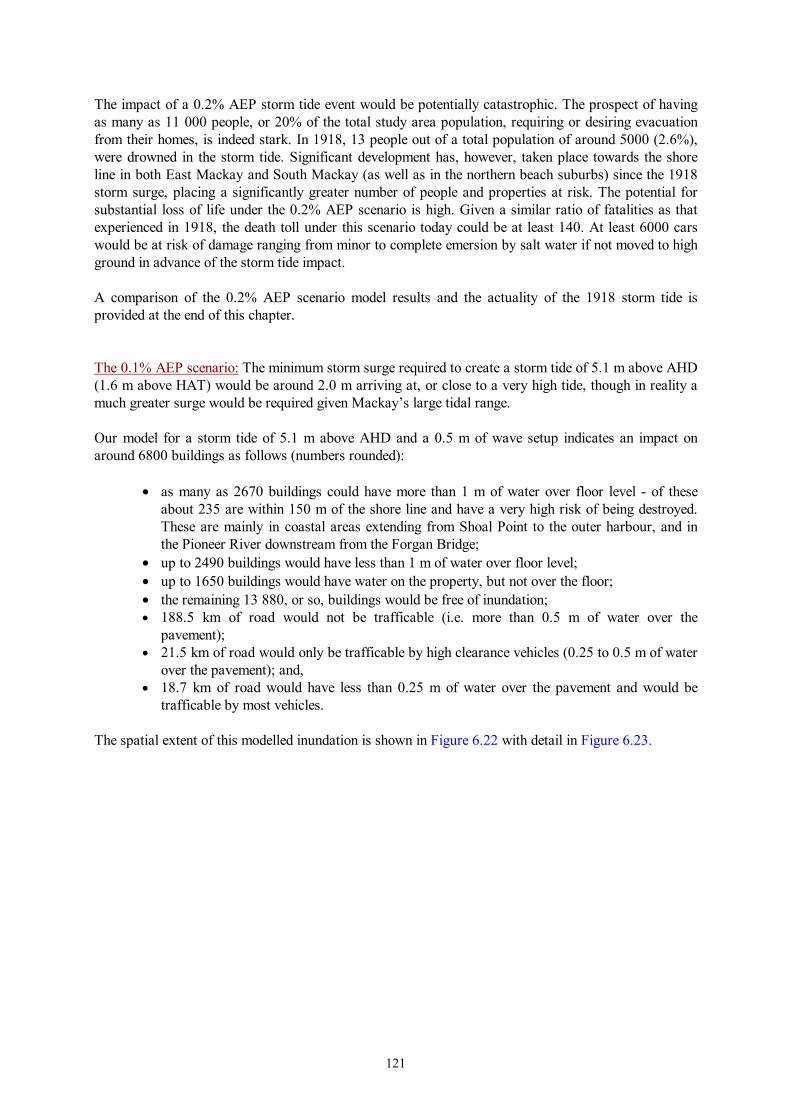
121

The impact of a 0.2% AEP storm tide event would be potentially catastrophic. The prospect of having as many as 11 000 people, or 20% of the total study area population, requiring or desiring evacuation from their homes, is indeed stark. In 1918, 13 people out of a total population of around 5000 (2.6%), were drowned in the storm tide. Significant development has, however, taken place towards the shore line in both East Mackay and South Mackay (as well as in the northern beach suburbs) since the 1918 storm surge, placing a significantly greater number of people and properties at risk. The potential for substantial loss of life under the 0.2% AEP scenario is high. Given a similar ratio of fatalities as that experienced in 1918, the death toll under this scenario today could be at least 140. At least 6000 cars would be at risk of damage ranging from minor to complete emersion by salt water if not moved to high ground in advance of the storm tide impact. A comparison of the 0.2% AEP scenario model results and the actuality of the 1918 storm tide is provided at the end of this chapter. The 0.1% AEP scenario: The minimum storm surge required to create a storm tide of 5.1 m above AHD (1.6 m above HAT) would be around 2.0 m arriving at, or close to a very high tide, though in reality a much greater surge would be required given Mackay’s large tidal range. Our model for a storm tide of 5.1 m above AHD and a 0.5 m of wave setup indicates an impact on around 6800 buildings as follows (numbers rounded):

• as many as 2670 buildings could have more than 1 m of water over floor level - of these about 235 are within 150 m of the shore line and have a very high risk of being destroyed. These are mainly in coastal areas extending from Shoal Point to the outer harbour, and in the Pioneer River downstream from the Forgan Bridge;

• up to 2490 buildings would have less than 1 m of water over floor level; • up to 1650 buildings would have water on the property, but not over the floor; • the remaining 13 880, or so, buildings would be free of inundation; • 188.5 km of road would not be trafficable (i.e. more than 0.5 m of water over the

pavement); • 21.5 km of road would only be trafficable by high clearance vehicles (0.25 to 0.5 m of water

over the pavement); and, • 18.7 km of road would have less than 0.25 m of water over the pavement and would be

trafficable by most vehicles. The spatial extent of this modelled inundation is shown in Figure 6.22 with detail in Figure 6.23.

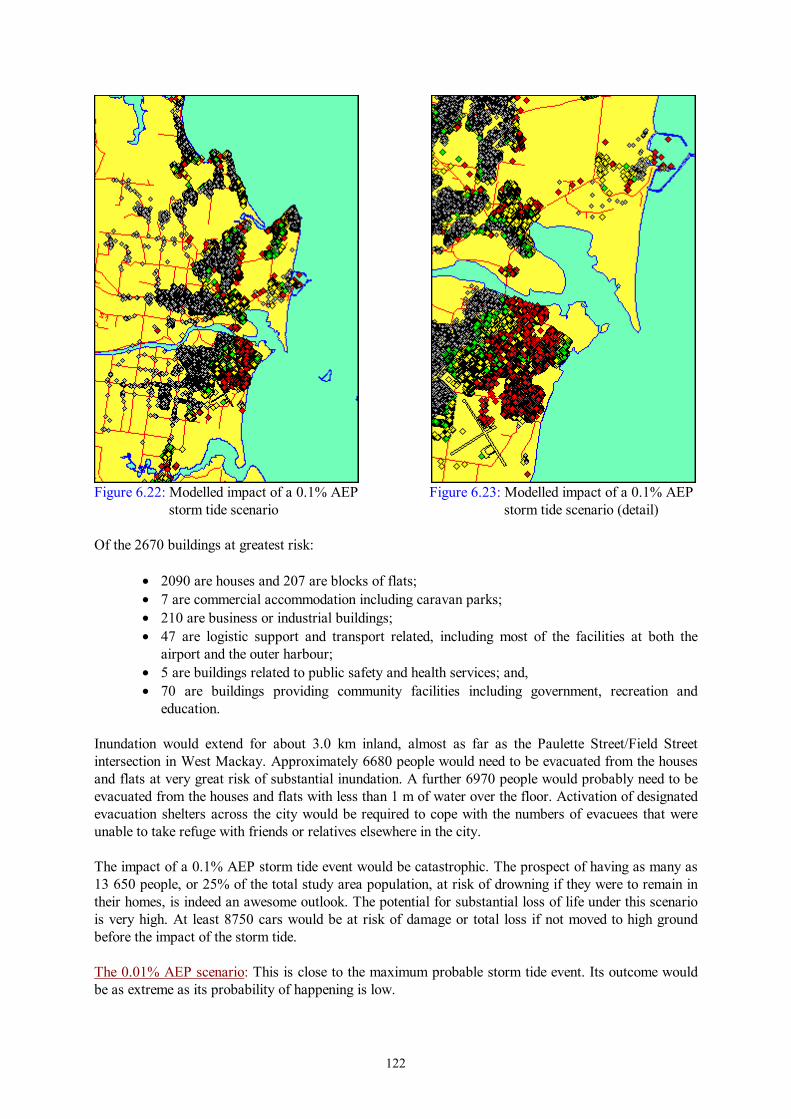
122

Figure 6.22: Modelled impact of a 0.1% AEP Figure 6.23: Modelled impact of a 0.1% AEP

storm tide scenario storm tide scenario (detail) Of the 2670 buildings at greatest risk:

• 2090 are houses and 207 are blocks of flats; • 7 are commercial accommodation including caravan parks; • 210 are business or industrial buildings; • 47 are logistic support and transport related, including most of the facilities at both the

airport and the outer harbour; • 5 are buildings related to public safety and health services; and, • 70 are buildings providing community facilities including government, recreation and

education. Inundation would extend for about 3.0 km inland, almost as far as the Paulette Street/Field Street intersection in West Mackay. Approximately 6680 people would need to be evacuated from the houses and flats at very great risk of substantial inundation. A further 6970 people would probably need to be evacuated from the houses and flats with less than 1 m of water over the floor. Activation of designated evacuation shelters across the city would be required to cope with the numbers of evacuees that were unable to take refuge with friends or relatives elsewhere in the city. The impact of a 0.1% AEP storm tide event would be catastrophic. The prospect of having as many as 13 650 people, or 25% of the total study area population, at risk of drowning if they were to remain in their homes, is indeed an awesome outlook. The potential for substantial loss of life under this scenario is very high. At least 8750 cars would be at risk of damage or total loss if not moved to high ground before the impact of the storm tide. The 0.01% AEP scenario: This is close to the maximum probable storm tide event. Its outcome would be as extreme as its probability of happening is low.

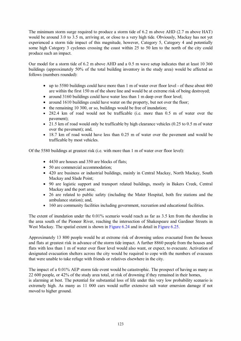
123

The minimum storm surge required to produce a storm tide of 6.2 m above AHD (2.7 m above HAT) would be around 3.0 to 3.5 m, arriving at, or close to a very high tide. Obviously, Mackay has not yet experienced a storm tide impact of this magnitude, however, Category 5, Category 4 and potentially some high Category 3 cyclones crossing the coast within 25 to 50 km to the north of the city could produce such an impact. Our model for a storm tide of 6.2 m above AHD and a 0.5 m wave setup indicates that at least 10 360 buildings (approximately 50% of the total building inventory in the study area) would be affected as follows (numbers rounded):

• up to 5580 buildings could have more than 1 m of water over floor level - of these about 460 are within the first 150 m of the shore line and would be at extreme risk of being destroyed;

• around 3160 buildings could have water less than 1 m deep over floor level; • around 1610 buildings could have water on the property, but not over the floor; • the remaining 10 300, or so, buildings would be free of inundation; • 282.4 km of road would not be trafficable (i.e. more than 0.5 m of water over the

pavement); • 21.5 km of road would only be trafficable by high clearance vehicles (0.25 to 0.5 m of water

over the pavement); and, • 18.7 km of road would have less than 0.25 m of water over the pavement and would be

trafficable by most vehicles. Of the 5580 buildings at greatest risk (i.e. with more than 1 m of water over floor level):

• 4430 are houses and 350 are blocks of flats; • 50 are commercial accommodation; • 420 are business or industrial buildings, mainly in Central Mackay, North Mackay, South

Mackay and Slade Point; • 90 are logistic support and transport related buildings, mostly in Bakers Creek, Central

Mackay and the port area; • 26 are related to public safety (including the Mater Hospital, both fire stations and the

ambulance station); and, • 160 are community facilities including government, recreation and educational facilities.

The extent of inundation under the 0.01% scenario would reach as far as 3.5 km from the shoreline in the area south of the Pioneer River, reaching the intersection of Shakespeare and Gardiner Streets in West Mackay. The spatial extent is shown in Figure 6.24 and in detail in Figure 6.25. Approximately 13 800 people would be at extreme risk of drowning unless evacuated from the houses and flats at greatest risk in advance of the storm tide impact. A further 8860 people from the houses and flats with less than 1 m of water over floor level would also want, or expect, to evacuate. Activation of designated evacuation shelters across the city would be required to cope with the numbers of evacuees that were unable to take refuge with friends or relatives elsewhere in the city. The impact of a 0.01% AEP storm tide event would be catastrophic. The prospect of having as many as 22 600 people, or 42% of the study area total, at risk of drowning if they remained in their homes, is alarming at best. The potential for substantial loss of life under this very low probability scenario is extremely high. As many as 11 000 cars would suffer extensive salt water emersion damage if not moved to higher ground.

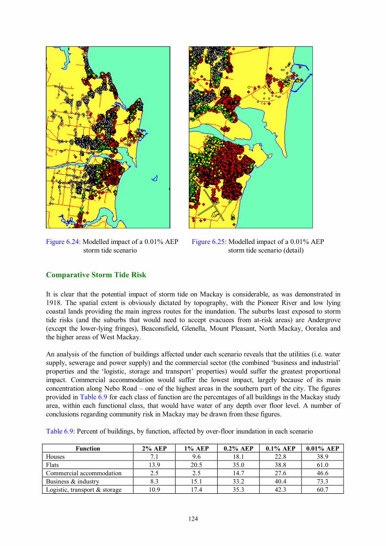
124

Figure 6.24: Modelled impact of a 0.01% AEP Figure 6.25: Modelled impact of a 0.01% AEP storm tide scenario storm tide scenario (detail)

Comparative Storm Tide Risk It is clear that the potential impact of storm tide on Mackay is considerable, as was demonstrated in 1918. The spatial extent is obviously dictated by topography, with the Pioneer River and low lying coastal lands providing the main ingress routes for the inundation. The suburbs least exposed to storm tide risks (and the suburbs that would need to accept evacuees from at-risk areas) are Andergrove (except the lower-lying fringes), Beaconsfield, Glenella, Mount Pleasant, North Mackay, Ooralea and the higher areas of West Mackay. An analysis of the function of buildings affected under each scenario reveals that the utilities (i.e. water supply, sewerage and power supply) and the commercial sector (the combined ‘business and industrial’ properties and the ‘logistic, storage and transport’ properties) would suffer the greatest proportional impact. Commercial accommodation would suffer the lowest impact, largely because of its main concentration along Nebo Road – one of the highest areas in the southern part of the city. The figures provided in Table 6.9 for each class of function are the percentages of all buildings in the Mackay study area, within each functional class, that would have water of any depth over floor level. A number of conclusions regarding community risk in Mackay may be drawn from these figures. Table 6.9: Percent of buildings, by function, affected by over-floor inundation in each scenario

Function 2% AEP 1% AEP 0.2% AEP 0.1% AEP 0.01% AEP Houses 7.1 9.6 18.1 22.8 38.9 Flats 13.9 20.5 35.0 38.8 61.0 Commercial accommodation 2.5 2.5 14.7 27.6 46.6 Business & industry 8.3 15.1 33.2 40.4 73.3 Logistic, transport & storage 10.9 17.4 35.3 42.3 60.7

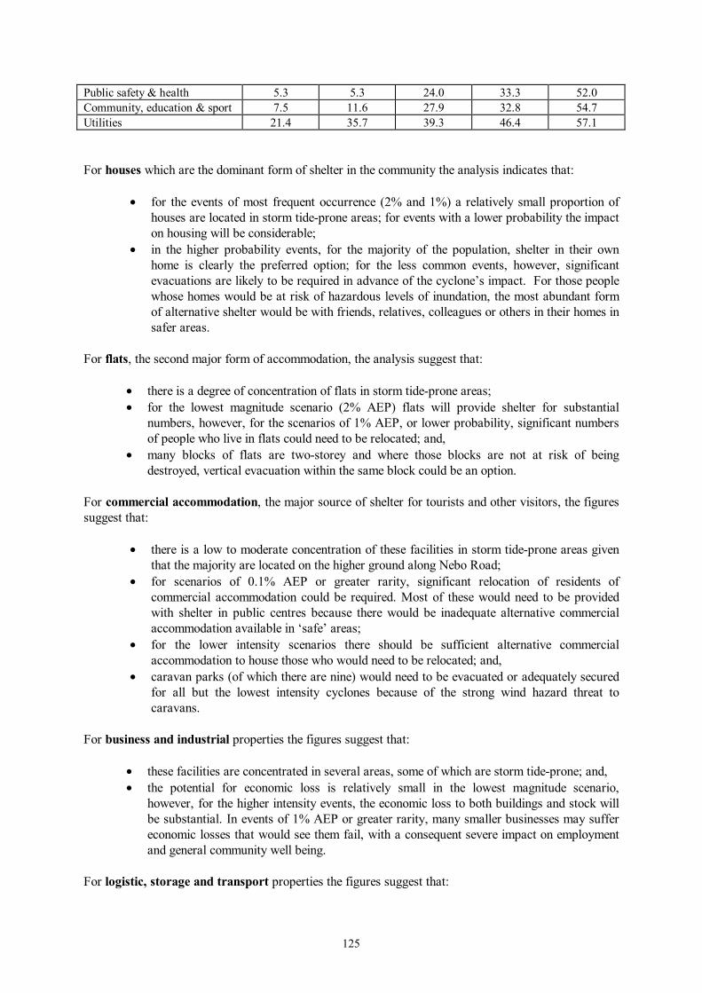
125

Public safety & health 5.3 5.3 24.0 33.3 52.0 Community, education & sport 7.5 11.6 27.9 32.8 54.7 Utilities 21.4 35.7 39.3 46.4 57.1 For houses which are the dominant form of shelter in the community the analysis indicates that:

• for the events of most frequent occurrence (2% and 1%) a relatively small proportion of houses are located in storm tide-prone areas; for events with a lower probability the impact on housing will be considerable;

• in the higher probability events, for the majority of the population, shelter in their own home is clearly the preferred option; for the less common events, however, significant evacuations are likely to be required in advance of the cyclone’s impact. For those people whose homes would be at risk of hazardous levels of inundation, the most abundant form of alternative shelter would be with friends, relatives, colleagues or others in their homes in safer areas.

For flats, the second major form of accommodation, the analysis suggest that:

• there is a degree of concentration of flats in storm tide-prone areas; • for the lowest magnitude scenario (2% AEP) flats will provide shelter for substantial

numbers, however, for the scenarios of 1% AEP, or lower probability, significant numbers of people who live in flats could need to be relocated; and,

• many blocks of flats are two-storey and where those blocks are not at risk of being destroyed, vertical evacuation within the same block could be an option.

For commercial accommodation, the major source of shelter for tourists and other visitors, the figures suggest that:

• there is a low to moderate concentration of these facilities in storm tide-prone areas given that the majority are located on the higher ground along Nebo Road;

• for scenarios of 0.1% AEP or greater rarity, significant relocation of residents of commercial accommodation could be required. Most of these would need to be provided with shelter in public centres because there would be inadequate alternative commercial accommodation available in ‘safe’ areas;

• for the lower intensity scenarios there should be sufficient alternative commercial accommodation to house those who would need to be relocated; and,

• caravan parks (of which there are nine) would need to be evacuated or adequately secured for all but the lowest intensity cyclones because of the strong wind hazard threat to caravans.

For business and industrial properties the figures suggest that:

• these facilities are concentrated in several areas, some of which are storm tide-prone; and, • the potential for economic loss is relatively small in the lowest magnitude scenario,

however, for the higher intensity events, the economic loss to both buildings and stock will be substantial. In events of 1% AEP or greater rarity, many smaller businesses may suffer economic losses that would see them fail, with a consequent severe impact on employment and general community well being.

For logistic, storage and transport properties the figures suggest that:

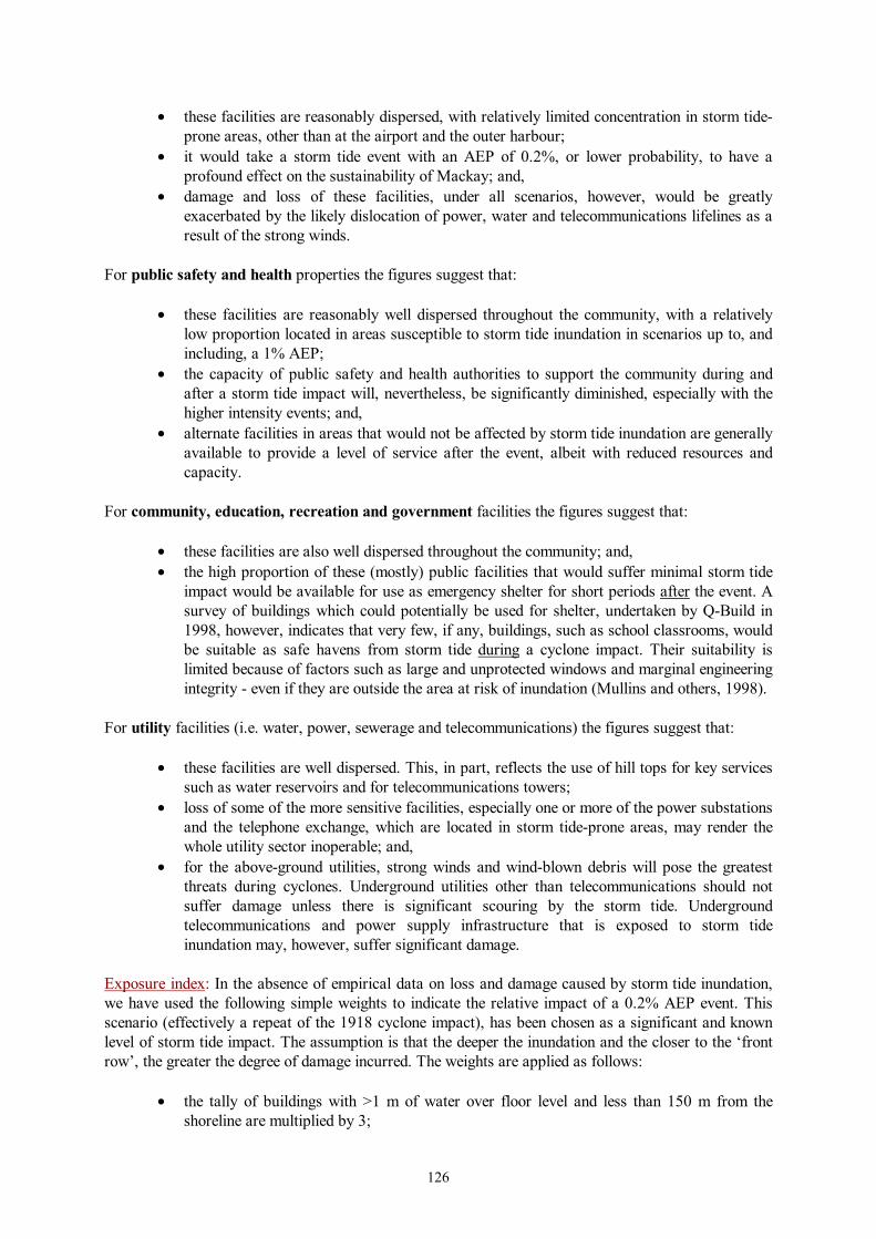
126

• these facilities are reasonably dispersed, with relatively limited concentration in storm tide-prone areas, other than at the airport and the outer harbour;

• it would take a storm tide event with an AEP of 0.2%, or lower probability, to have a profound effect on the sustainability of Mackay; and,

• damage and loss of these facilities, under all scenarios, however, would be greatly exacerbated by the likely dislocation of power, water and telecommunications lifelines as a result of the strong winds.

For public safety and health properties the figures suggest that:

• these facilities are reasonably well dispersed throughout the community, with a relatively low proportion located in areas susceptible to storm tide inundation in scenarios up to, and including, a 1% AEP;

• the capacity of public safety and health authorities to support the community during and after a storm tide impact will, nevertheless, be significantly diminished, especially with the higher intensity events; and,

• alternate facilities in areas that would not be affected by storm tide inundation are generally available to provide a level of service after the event, albeit with reduced resources and capacity.

For community, education, recreation and government facilities the figures suggest that:

• these facilities are also well dispersed throughout the community; and, • the high proportion of these (mostly) public facilities that would suffer minimal storm tide

impact would be available for use as emergency shelter for short periods after the event. A survey of buildings which could potentially be used for shelter, undertaken by Q-Build in 1998, however, indicates that very few, if any, buildings, such as school classrooms, would be suitable as safe havens from storm tide during a cyclone impact. Their suitability is limited because of factors such as large and unprotected windows and marginal engineering integrity - even if they are outside the area at risk of inundation (Mullins and others, 1998).

For utility facilities (i.e. water, power, sewerage and telecommunications) the figures suggest that:

• these facilities are well dispersed. This, in part, reflects the use of hill tops for key services such as water reservoirs and for telecommunications towers;

• loss of some of the more sensitive facilities, especially one or more of the power substations and the telephone exchange, which are located in storm tide-prone areas, may render the whole utility sector inoperable; and,

• for the above-ground utilities, strong winds and wind-blown debris will pose the greatest threats during cyclones. Underground utilities other than telecommunications should not suffer damage unless there is significant scouring by the storm tide. Underground telecommunications and power supply infrastructure that is exposed to storm tide inundation may, however, suffer significant damage.

Exposure index: In the absence of empirical data on loss and damage caused by storm tide inundation, we have used the following simple weights to indicate the relative impact of a 0.2% AEP event. This scenario (effectively a repeat of the 1918 cyclone impact), has been chosen as a significant and known level of storm tide impact. The assumption is that the deeper the inundation and the closer to the ‘front row’, the greater the degree of damage incurred. The weights are applied as follows:

• the tally of buildings with >1 m of water over floor level and less than 150 m from the shoreline are multiplied by 3;

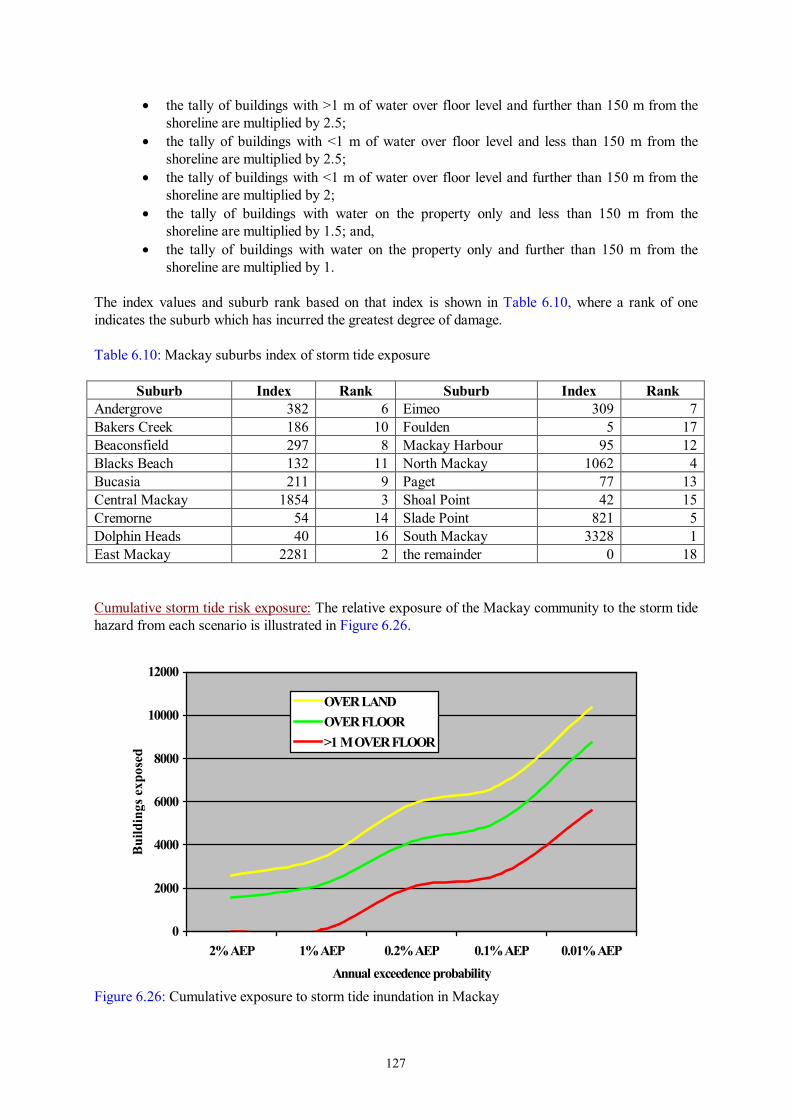
127

• the tally of buildings with >1 m of water over floor level and further than 150 m from the shoreline are multiplied by 2.5;

• the tally of buildings with <1 m of water over floor level and less than 150 m from the shoreline are multiplied by 2.5;

• the tally of buildings with <1 m of water over floor level and further than 150 m from the shoreline are multiplied by 2;

• the tally of buildings with water on the property only and less than 150 m from the shoreline are multiplied by 1.5; and,

• the tally of buildings with water on the property only and further than 150 m from the shoreline are multiplied by 1.

The index values and suburb rank based on that index is shown in Table 6.10, where a rank of one indicates the suburb which has incurred the greatest degree of damage. Table 6.10: Mackay suburbs index of storm tide exposure

Suburb Index Rank Suburb Index Rank Andergrove 382 6 Eimeo 309 7Bakers Creek 186 10 Foulden 5 17Beaconsfield 297 8 Mackay Harbour 95 12Blacks Beach 132 11 North Mackay 1062 4Bucasia 211 9 Paget 77 13Central Mackay 1854 3 Shoal Point 42 15Cremorne 54 14 Slade Point 821 5Dolphin Heads 40 16 South Mackay 3328 1East Mackay 2281 2 the remainder 0 18 Cumulative storm tide risk exposure: The relative exposure of the Mackay community to the storm tide hazard from each scenario is illustrated in Figure 6.26.

Figure 6.26: Cumulative exposure to storm tide inundation in Mackay

0

2000

4000

6000

8000

10000

12000

2% AEP 1% AEP 0.2% AEP 0.1% AEP 0.01% AEPAnnual exceedence probability

Build

ings

exp

osed

OVER LANDOVER FLOOR>1 M OVER FLOOR

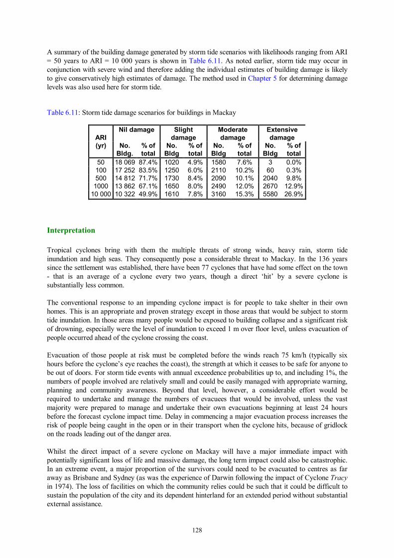
128

A summary of the building damage generated by storm tide scenarios with likelihoods ranging from ARI = 50 years to ARI = 10 000 years is shown in Table 6.11. As noted earlier, storm tide may occur in conjunction with severe wind and therefore adding the individual estimates of building damage is likely to give conservatively high estimates of damage. The method used in Chapter 5 for determining damage levels was also used here for storm tide. Table 6.11: Storm tide damage scenarios for buildings in Mackay

ARI

Nil damage Slight damage

Moderate damage

Extensive damage

(yr) No. Bldg.

% of total

No. Bldg

% of total

No. Bldg

% of total

No. Bldg

% of total

50 18 069 87.4% 1020 4.9% 1580 7.6% 3 0.0% 100 17 252 83.5% 1250 6.0% 2110 10.2% 60 0.3% 500 14 812 71.7% 1730 8.4% 2090 10.1% 2040 9.8%

1000 13 862 67.1% 1650 8.0% 2490 12.0% 2670 12.9% 10 000 10 322 49.9% 1610 7.8% 3160 15.3% 5580 26.9%

Interpretation Tropical cyclones bring with them the multiple threats of strong winds, heavy rain, storm tide inundation and high seas. They consequently pose a considerable threat to Mackay. In the 136 years since the settlement was established, there have been 77 cyclones that have had some effect on the town - that is an average of a cyclone every two years, though a direct ‘hit’ by a severe cyclone is substantially less common. The conventional response to an impending cyclone impact is for people to take shelter in their own homes. This is an appropriate and proven strategy except in those areas that would be subject to storm tide inundation. In those areas many people would be exposed to building collapse and a significant risk of drowning, especially were the level of inundation to exceed 1 m over floor level, unless evacuation of people occurred ahead of the cyclone crossing the coast. Evacuation of those people at risk must be completed before the winds reach 75 km/h (typically six hours before the cyclone’s eye reaches the coast), the strength at which it ceases to be safe for anyone to be out of doors. For storm tide events with annual exceedence probabilities up to, and including 1%, the numbers of people involved are relatively small and could be easily managed with appropriate warning, planning and community awareness. Beyond that level, however, a considerable effort would be required to undertake and manage the numbers of evacuees that would be involved, unless the vast majority were prepared to manage and undertake their own evacuations beginning at least 24 hours before the forecast cyclone impact time. Delay in commencing a major evacuation process increases the risk of people being caught in the open or in their transport when the cyclone hits, because of gridlock on the roads leading out of the danger area. Whilst the direct impact of a severe cyclone on Mackay will have a major immediate impact with potentially significant loss of life and massive damage, the long term impact could also be catastrophic. In an extreme event, a major proportion of the survivors could need to be evacuated to centres as far away as Brisbane and Sydney (as was the experience of Darwin following the impact of Cyclone Tracy in 1974). The loss of facilities on which the community relies could be such that it could be difficult to sustain the population of the city and its dependent hinterland for an extended period without substantial external assistance.

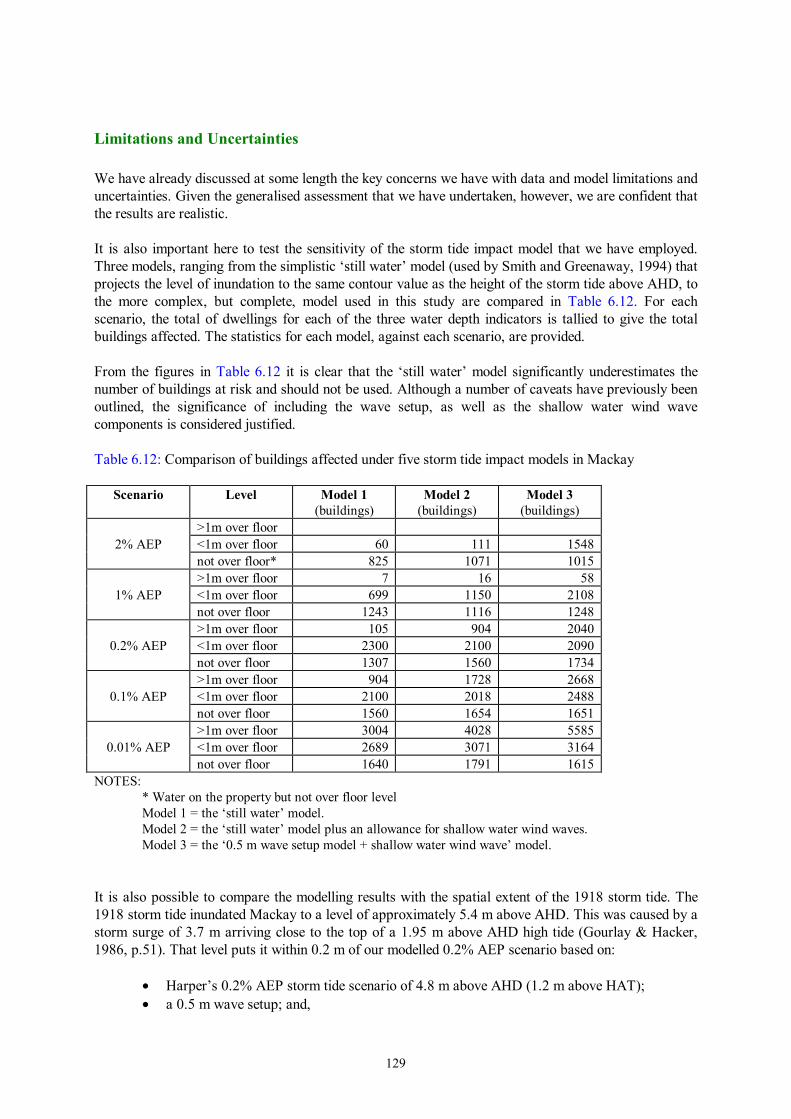
129

Limitations and Uncertainties We have already discussed at some length the key concerns we have with data and model limitations and uncertainties. Given the generalised assessment that we have undertaken, however, we are confident that the results are realistic. It is also important here to test the sensitivity of the storm tide impact model that we have employed. Three models, ranging from the simplistic ‘still water’ model (used by Smith and Greenaway, 1994) that projects the level of inundation to the same contour value as the height of the storm tide above AHD, to the more complex, but complete, model used in this study are compared in Table 6.12. For each scenario, the total of dwellings for each of the three water depth indicators is tallied to give the total buildings affected. The statistics for each model, against each scenario, are provided. From the figures in Table 6.12 it is clear that the ‘still water’ model significantly underestimates the number of buildings at risk and should not be used. Although a number of caveats have previously been outlined, the significance of including the wave setup, as well as the shallow water wind wave components is considered justified. Table 6.12: Comparison of buildings affected under five storm tide impact models in Mackay

Scenario Level Model 1 (buildings)

Model 2 (buildings)

Model 3 (buildings)

>1m over floor 2% AEP <1m over floor 60 111 1548

not over floor* 825 1071 1015 >1m over floor 7 16 58

1% AEP <1m over floor 699 1150 2108 not over floor 1243 1116 1248 >1m over floor 105 904 2040

0.2% AEP <1m over floor 2300 2100 2090 not over floor 1307 1560 1734 >1m over floor 904 1728 2668

0.1% AEP <1m over floor 2100 2018 2488 not over floor 1560 1654 1651 >1m over floor 3004 4028 5585

0.01% AEP <1m over floor 2689 3071 3164 not over floor 1640 1791 1615 NOTES:

* Water on the property but not over floor level Model 1 = the ‘still water’ model. Model 2 = the ‘still water’ model plus an allowance for shallow water wind waves. Model 3 = the ‘0.5 m wave setup model + shallow water wind wave’ model.

It is also possible to compare the modelling results with the spatial extent of the 1918 storm tide. The 1918 storm tide inundated Mackay to a level of approximately 5.4 m above AHD. This was caused by a storm surge of 3.7 m arriving close to the top of a 1.95 m above AHD high tide (Gourlay & Hacker, 1986, p.51). That level puts it within 0.2 m of our modelled 0.2% AEP scenario based on:

• Harper’s 0.2% AEP storm tide scenario of 4.8 m above AHD (1.2 m above HAT); • a 0.5 m wave setup; and,

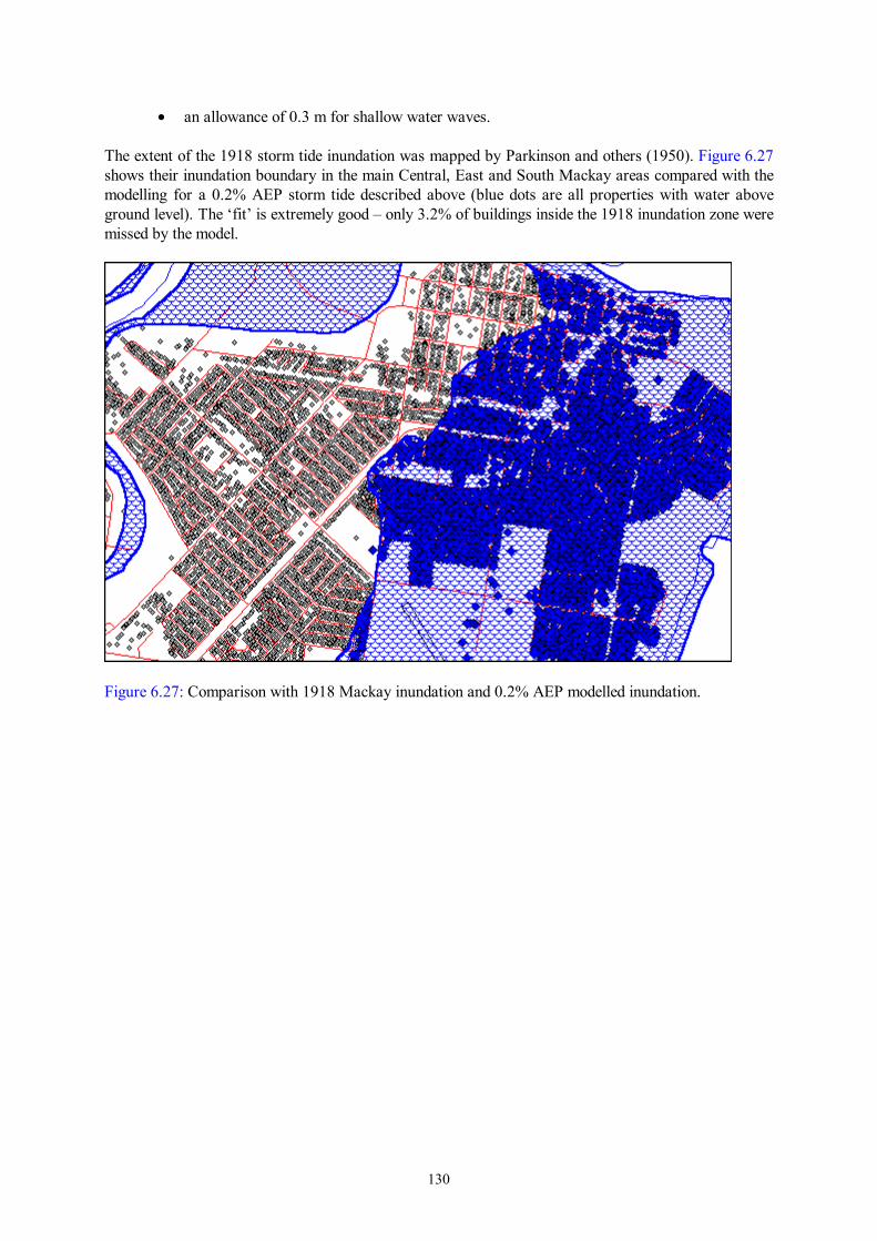
130

• an allowance of 0.3 m for shallow water waves. The extent of the 1918 storm tide inundation was mapped by Parkinson and others (1950). Figure 6.27 shows their inundation boundary in the main Central, East and South Mackay areas compared with the modelling for a 0.2% AEP storm tide described above (blue dots are all properties with water above ground level). The ‘fit’ is extremely good – only 3.2% of buildings inside the 1918 inundation zone were missed by the model.

Figure 6.27: Comparison with 1918 Mackay inundation and 0.2% AEP modelled inundation.