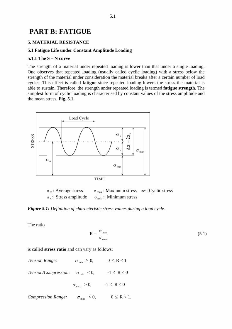
5.1

PART B: FATIGUE 5. MATERIAL RESISTANCE

5.1 Fatigue Life under Constant Amplitude Loading

5.1.1 The S – N curve

The strength of a material under repeated loading is lower than that under a single loading. One observes that repeated loading (usually called cyclic loading) with a stress below the strength of the material under consideration the material breaks after a certain number of load cycles. This effect is called fatigue since repeated loading lowers the stress the material is able to sustain. Therefore, the strength under repeated loading is termed fatigue strength. The simplest form of cyclic loading is characterised by constant values of the stress amplitude and the mean stress, Fig. 5.1.

mσ : Average stress maxσ : Maximum stress σ∆ : Cyclic stress aσ : Stress amplitude minσ : Minimum stress Figure 5.1: Definition of characteristic stress values during a load cycle. The ratio

R = max

min

σσ (5.1)

is called stress ratio and can vary as follows: Tension Range: minσ ≥ 0, 0 ≤ R < 1 Tension/Compression: minσ < 0, -1 < R < 0 maxσ > 0, -1 < R < 0 Compression Range: maxσ < 0, 0 ≤ R < 1.

5.2

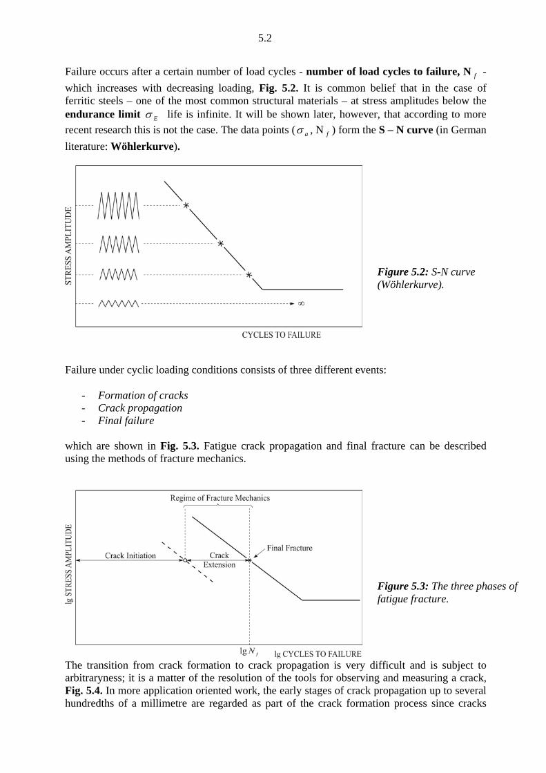
Failure occurs after a certain number of load cycles - number of load cycles to failure, N f - which increases with decreasing loading, Fig. 5.2. It is common belief that in the case of ferritic steels – one of the most common structural materials – at stress amplitudes below the endurance limit Eσ life is infinite. It will be shown later, however, that according to more recent research this is not the case. The data points ( aσ , N f ) form the S – N curve (in German literature: Wöhlerkurve).

Failure under cyclic loading conditions consists of three different events:

- Formation of cracks - Crack propagation - Final failure

which are shown in Fig. 5.3. Fatigue crack propagation and final fracture can be described using the methods of fracture mechanics.

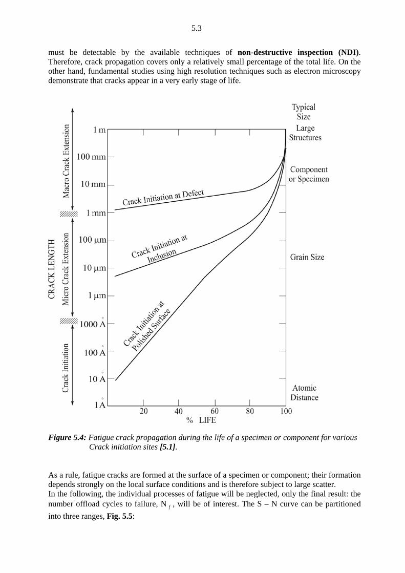
The transition from crack formation to crack propagation is very difficult and is subject to arbitraryness; it is a matter of the resolution of the tools for observing and measuring a crack, Fig. 5.4. In more application oriented work, the early stages of crack propagation up to several hundredths of a millimetre are regarded as part of the crack formation process since cracks

Figure 5.2: S-N curve (Wöhlerkurve).

Figure 5.3: The three phases of fatigue fracture.

5.3

must be detectable by the available techniques of non-destructive inspection (NDI). Therefore, crack propagation covers only a relatively small percentage of the total life. On the other hand, fundamental studies using high resolution techniques such as electron microscopy demonstrate that cracks appear in a very early stage of life.

Figure 5.4: Fatigue crack propagation during the life of a specimen or component for various Crack initiation sites [5.1]. As a rule, fatigue cracks are formed at the surface of a specimen or component; their formation depends strongly on the local surface conditions and is therefore subject to large scatter. In the following, the individual processes of fatigue will be neglected, only the final result: the number offload cycles to failure, N f , will be of interest. The S – N curve can be partitioned into three ranges, Fig. 5.5:

5.4

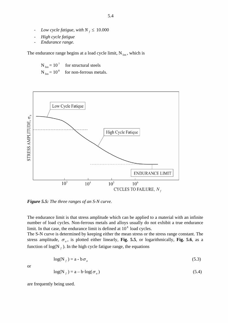
- Low cycle fatigue, with N f ≤ 10.000 - High cycle fatigue - Endurance range.

The endurance range begins at a load cycle limit, N lim , which is N lim = 10 7 for structural steels N lim = 10 8 for non-ferrous metals.

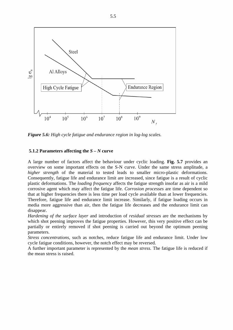
Figure 5.5: The three ranges of an S-N curve. The endurance limit is that stress amplitude which can be applied to a material with an infinite number of load cycles. Non-ferrous metals and alloys usually do not exhibit a true endurance limit. In that case, the endurance limit is defined at 10 8 load cycles. The S-N curve is determined by keeping either the mean stress or the stress range constant. The stress amplitude, aσ , is plotted either linearly, Fig. 5.5, or logarithmically, Fig. 5.6, as a function of log(N f ). In the high cycle fatigue range, the equations log(N f ) = a - b aσ (5.3) or log(N f ) = a – b·log( aσ ) (5.4) are frequently being used.

5.5

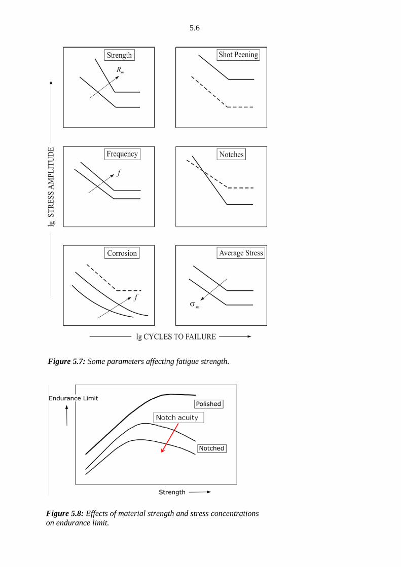
Figure 5.6: High cycle fatigue and endurance region in log-log scales. 5.1.2 Parameters affecting the S – N curve A large number of factors affect the behaviour under cyclic loading. Fig. 5.7 provides an overview on some important effects on the S-N curve. Under the same stress amplitude, a higher strength of the material to tested leads to smaller micro-plastic deformations. Consequently, fatigue life and endurance limit are increased, since fatigue is a result of cyclic plastic deformations. The loading frequency affects the fatigue strength insofar as air is a mild corrosive agent which may affect the fatigue life. Corrosion processes are time dependent so that at higher frequencies there is less time per load cycle available than at lower frequencies. Therefore, fatigue life and endurance limit increase. Similarly, if fatigue loading occurs in media more aggressive than air, then the fatigue life decreases and the endurance limit can disappear. Hardening of the surface layer and introduction of residual stresses are the mechanisms by which shot peening improves the fatigue properties. However, this very positive effect can be partially or entirely removed if shot peening is carried out beyond the optimum peening parameters. Stress concentrations, such as notches, reduce fatigue life and endurance limit. Under low cycle fatigue conditions, however, the notch effect may be reversed. A further important parameter is represented by the mean stress. The fatigue life is reduced if the mean stress is raised.

5.6

Figure 5.7: Some parameters affecting fatigue strength.

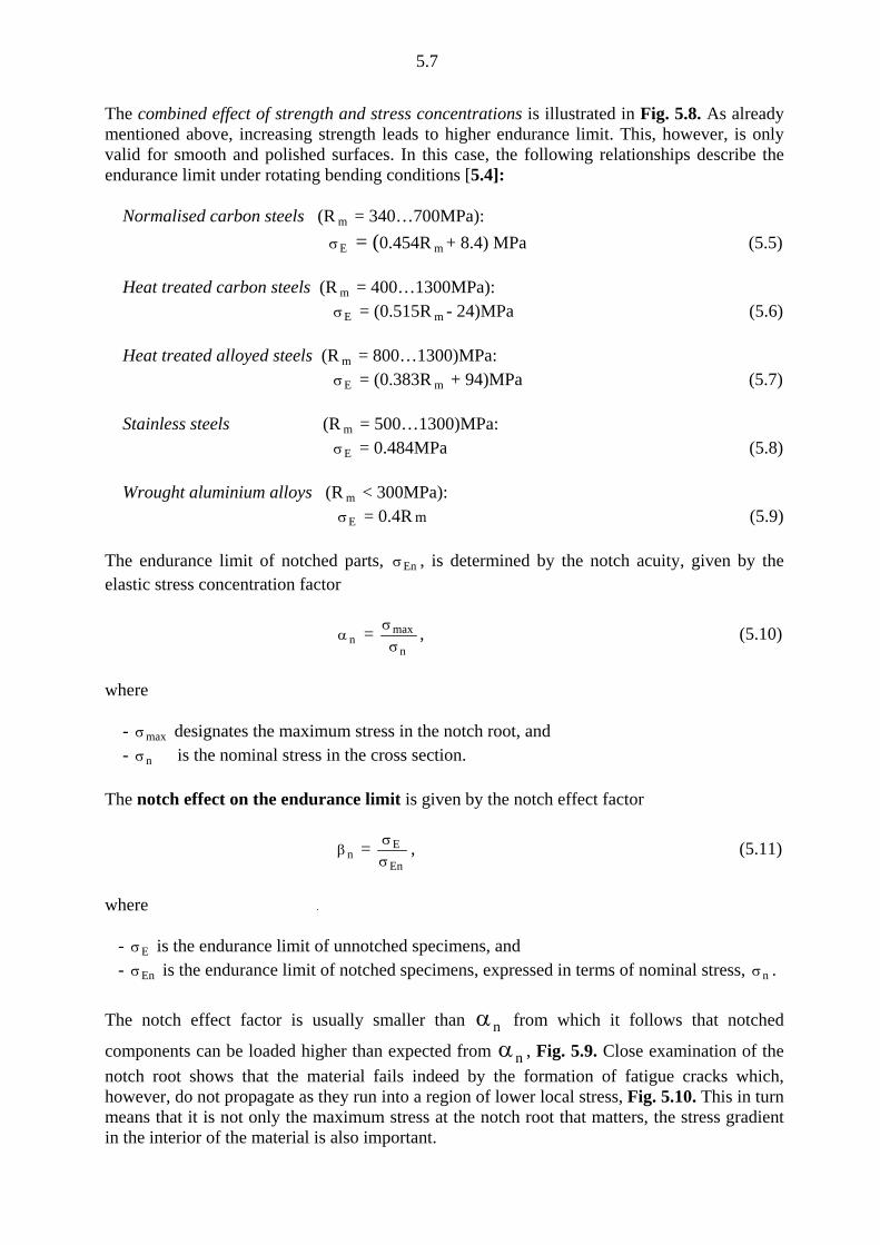
Figure 5.8: Effects of material strength and stress concentrations on endurance limit.

5.7

The combined effect of strength and stress concentrations is illustrated in Fig. 5.8. As already mentioned above, increasing strength leads to higher endurance limit. This, however, is only valid for smooth and polished surfaces. In this case, the following relationships describe the endurance limit under rotating bending conditions [5.4]: Normalised carbon steels (R m = 340…700MPa): Eσ = (0.454R m + 8.4) MPa (5.5) Heat treated carbon steels (R m = 400…1300MPa): Eσ = (0.515R m - 24)MPa (5.6) Heat treated alloyed steels (R m = 800…1300)MPa: Eσ = (0.383R m + 94)MPa (5.7) Stainless steels (R m = 500…1300)MPa: Eσ = 0.484MPa (5.8) Wrought aluminium alloys (R m < 300MPa): Eσ = 0.4R m (5.9) The endurance limit of notched parts, Enσ , is determined by the notch acuity, given by the elastic stress concentration factor

nα = n

maxσσ , (5.10)

where - maxσ designates the maximum stress in the notch root, and - nσ is the nominal stress in the cross section. The notch effect on the endurance limit is given by the notch effect factor

nβ = En

Eσσ , (5.11)

where - Eσ is the endurance limit of unnotched specimens, and - Enσ is the endurance limit of notched specimens, expressed in terms of nominal stress, nσ . The notch effect factor is usually smaller than nα from which it follows that notched

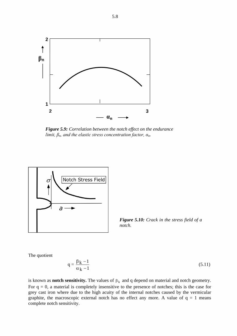
components can be loaded higher than expected from nα , Fig. 5.9. Close examination of the notch root shows that the material fails indeed by the formation of fatigue cracks which, however, do not propagate as they run into a region of lower local stress, Fig. 5.10. This in turn means that it is not only the maximum stress at the notch root that matters, the stress gradient in the interior of the material is also important.

5.8

The quotient

q = 1k

1k−α−β (5.11)

is known as notch sensitivity. The values of kβ and q depend on material and notch geometry. For q = 0, a material is completely insensitive to the presence of notches; this is the case for grey cast iron where due to the high acuity of the internal notches caused by the vermicular graphite, the macroscopic external notch has no effect any more. A value of q = 1 means complete notch sensitivity.

1

2

3 αn

βn

2

Figure 5.9: Correlation between the notch effect on the endurance limit, βn, and the elastic stress concentration factor, αn.

Figure 5.10: Crack in the stress field of a notch.

5.9

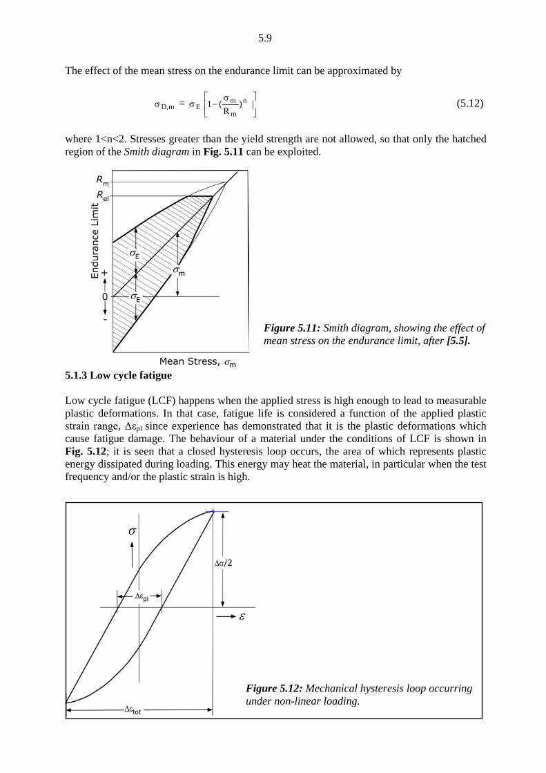
The effect of the mean stress on the endurance limit can be approximated by

m,Dσ = Eσ

σ− n

m

m )R

(1 (5.12)

where 1<n<2. Stresses greater than the yield strength are not allowed, so that only the hatched region of the Smith diagram in Fig. 5.11 can be exploited.

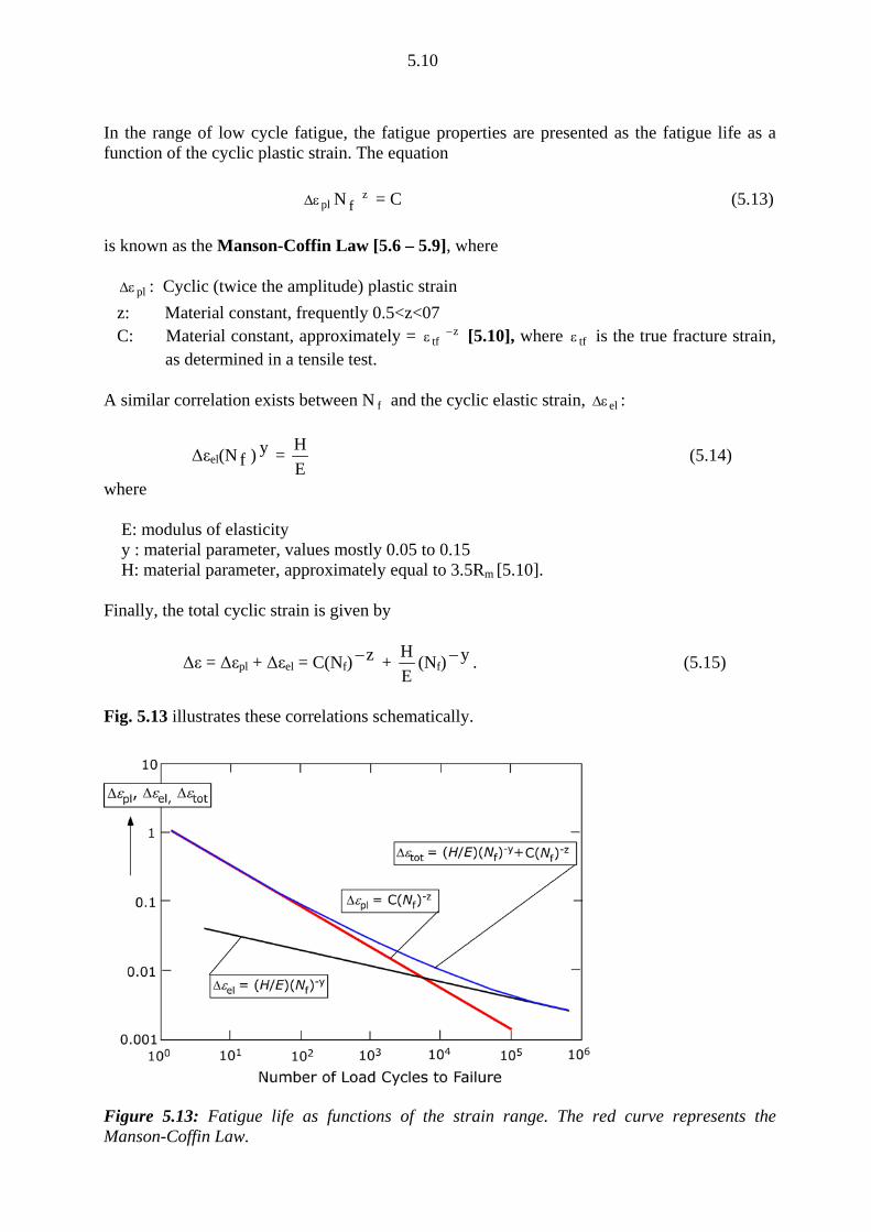
5.1.3 Low cycle fatigue Low cycle fatigue (LCF) happens when the applied stress is high enough to lead to measurable plastic deformations. In that case, fatigue life is considered a function of the applied plastic strain range, Δεpl since experience has demonstrated that it is the plastic deformations which cause fatigue damage. The behaviour of a material under the conditions of LCF is shown in Fig. 5.12; it is seen that a closed hysteresis loop occurs, the area of which represents plastic energy dissipated during loading. This energy may heat the material, in particular when the test frequency and/or the plastic strain is high.

Figure 5.12: Mechanical hysteresis loop occurring under non-linear loading.

Figure 5.11: Smith diagram, showing the effect of mean stress on the endurance limit, after [5.5].

5.10

In the range of low cycle fatigue, the fatigue properties are presented as the fatigue life as a function of the cyclic plastic strain. The equation plε∆ N f

z = C (5.13) is known as the Manson-Coffin Law [5.6 – 5.9], where plε∆ : Cyclic (twice the amplitude) plastic strain z: Material constant, frequently 0.5<z<07 C: Material constant, approximately = tfε z− [5.10], where tfε is the true fracture strain, as determined in a tensile test. A similar correlation exists between N f and the cyclic elastic strain, elε∆ :

Δεel(N f ) y = EH (5.14)

where E: modulus of elasticity y : material parameter, values mostly 0.05 to 0.15 H: material parameter, approximately equal to 3.5Rm [5.10]. Finally, the total cyclic strain is given by

Δε = Δεpl + Δεel = C(Nf) z− + EH (Nf) y− . (5.15)

Fig. 5.13 illustrates these correlations schematically.

Figure 5.13: Fatigue life as functions of the strain range. The red curve represents the Manson-Coffin Law.

5.11

At elevated temperatures creep may occur, which is a time dependant effect, thus leading to an influence of the frequency, υ, to fatigue life. A reasonable approach to accounting for this effect can be formulated by the following modification of Eq.(5.15) [5.10, 5.11]:

Δε = C(Nfυ a ) z− + EH [N f υ b ] y− (5.16)

where a and b are material parameters. 5.2 Fracture Mechanics Methods in Fatigue

5.2.1 Basic fatigue mechanisms

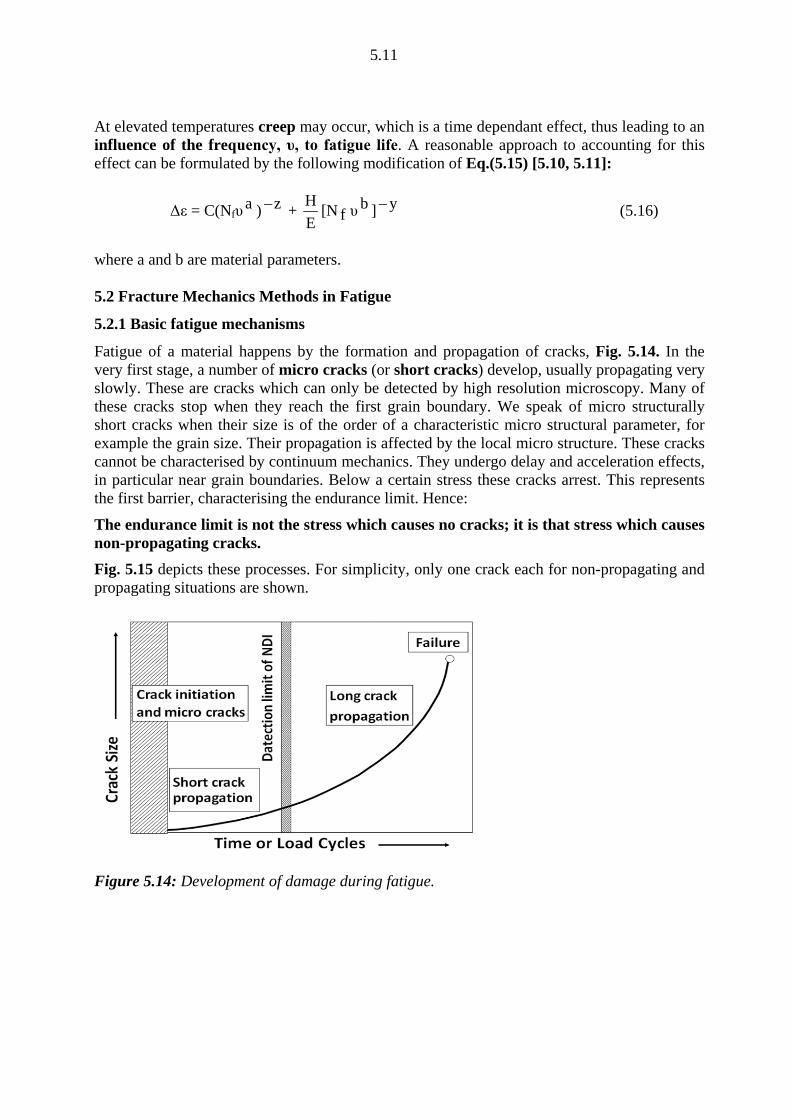
Fatigue of a material happens by the formation and propagation of cracks, Fig. 5.14. In the very first stage, a number of micro cracks (or short cracks) develop, usually propagating very slowly. These are cracks which can only be detected by high resolution microscopy. Many of these cracks stop when they reach the first grain boundary. We speak of micro structurally short cracks when their size is of the order of a characteristic micro structural parameter, for example the grain size. Their propagation is affected by the local micro structure. These cracks cannot be characterised by continuum mechanics. They undergo delay and acceleration effects, in particular near grain boundaries. Below a certain stress these cracks arrest. This represents the first barrier, characterising the endurance limit. Hence:

The endurance limit is not the stress which causes no cracks; it is that stress which causes non-propagating cracks. Fig. 5.15 depicts these processes. For simplicity, only one crack each for non-propagating and propagating situations are shown.

Figure 5.14: Development of damage during fatigue.

5.12

Figure 5.15: Fatigue crack propagation in relation to grain size.

5.2.2 Crack propagation diagram A few cracks are able to overcome the barrier of the first grain boundary, and eventually only one dominating crack – which is now a macro crack - propagates and may lead to final failure of the test piece or structural component.

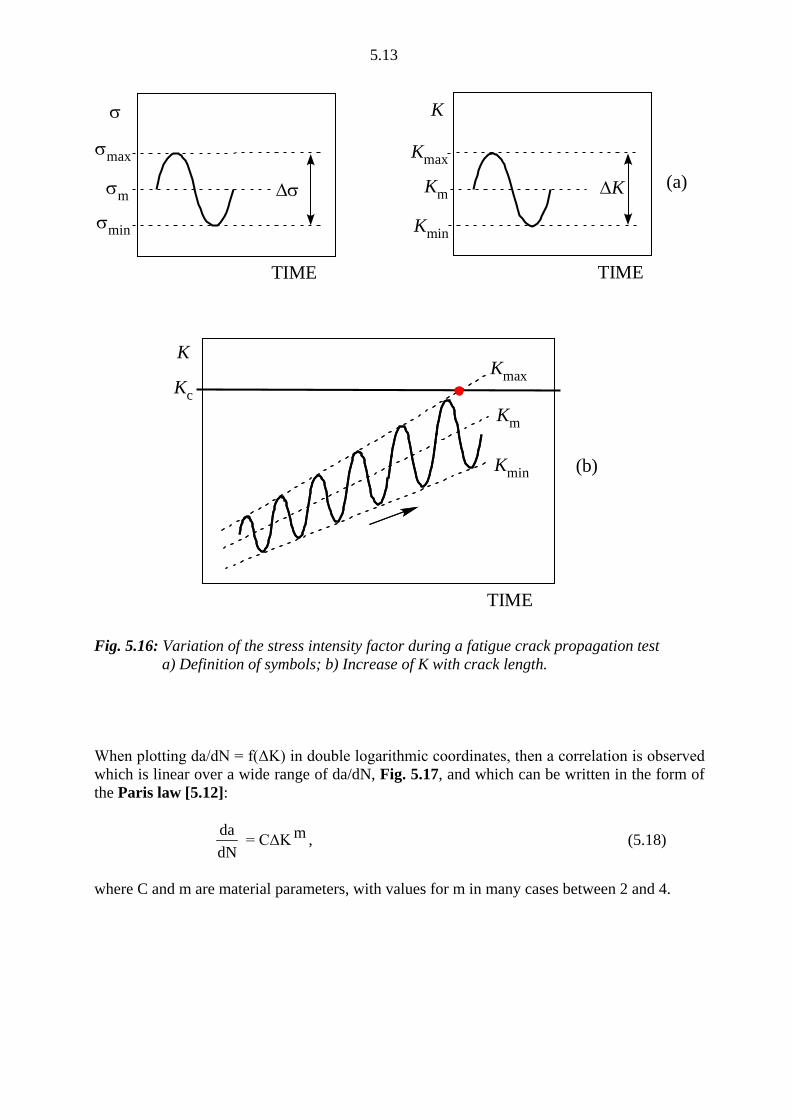
When investigating the propagation of fatigue cracks, the crack size, a, is measured as a function of the number of elapsed load cycles, and the crack propagation rate, da/dN is then calculated by point-wise differentiation of the a-N curve. The thus determined crack propagation rate is taken as a function of the cyclic stress intensity factor (or stress intensity range), ΔK, which is shown in Fig. 5.16. This is based on the idea that fatigue crack propagation is caused by cyclic plastic deformations at the crack tip which in turn are determined by the cyclic stress intensity factor. In most cases, fatigue crack propagation studies are performed under constant mean stress and constant stress amplitude conditions. In such tests, ΔK varies with the increasing crack length according to

ΔK = Δσ aπ Y(a/W) (5.17) as shown in Fig.5.16b. Final fracture occurs if either K max = K c , or if the condition of plastic collapse in the uncracked net section is reached (see end of 2.3.3). (These conditions are, of course, also valid for non-constant mean stress and stress amplitude tests).

5.13

(b)

TIME TIME

K

Kmax

Kmin

∆KKm(a)

σ

σmin

∆σσm

σmax

Kc

TIME

K

Kmin

Km

Kmax

Fig. 5.16: Variation of the stress intensity factor during a fatigue crack propagation test a) Definition of symbols; b) Increase of K with crack length. When plotting da/dN = f(ΔK) in double logarithmic coordinates, then a correlation is observed which is linear over a wide range of da/dN, Fig. 5.17, and which can be written in the form of the Paris law [5.12]:

dNda = CΔK m , (5.18)

where C and m are material parameters, with values for m in many cases between 2 and 4.

5.14

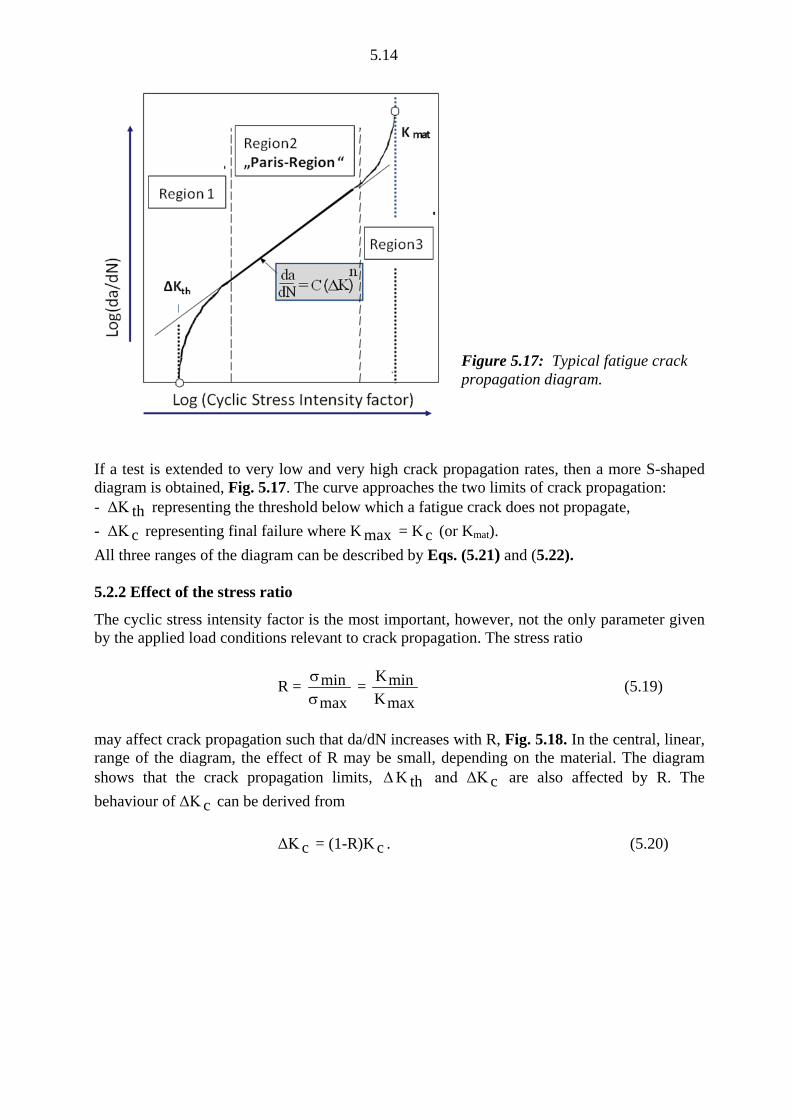
If a test is extended to very low and very high crack propagation rates, then a more S-shaped diagram is obtained, Fig. 5.17. The curve approaches the two limits of crack propagation: - ΔK th representing the threshold below which a fatigue crack does not propagate, - ΔK c representing final failure where K max = K c (or Kmat). All three ranges of the diagram can be described by Eqs. (5.21) and (5.22). 5.2.2 Effect of the stress ratio

The cyclic stress intensity factor is the most important, however, not the only parameter given by the applied load conditions relevant to crack propagation. The stress ratio

R = maxmin

σσ =

maxKminK (5.19)

may affect crack propagation such that da/dN increases with R, Fig. 5.18. In the central, linear, range of the diagram, the effect of R may be small, depending on the material. The diagram shows that the crack propagation limits, ∆K th and ΔK c are also affected by R. The behaviour of ΔK c can be derived from ΔK c = (1-R)K c . (5.20)

Figure 5.17: Typical fatigue crack propagation diagram.

5.15

The effect of R on the crack propagation rate has the consequence that the parameters C and m in Eq.(5.18) are no longer constant, but depend on R. Numerous attempts have been undertaken to describe this effect analytically by modifying Eq.(5.18). This way, C and m have to be determined for one R-value only and da/dN can then be predicted for other R-values by means of the modified equations. The most popular approach was presented by Forman et al. [5.13]:

dNda =

KcK)R1(

m)K(C∆−−

∆ = )maxKcK)(R1(

m)K(C−−

∆ . (5.21)

This equation serves two purposes: It describes the increase of da/dN with increasing R and the rapid increase of da/dN when K max → K c and is hence applicable to regions II and III of Fig. 5.18. Fig. 5.19 shows an example. With the following two modifications, region I can also be modelled:

KcK)R1(

m)thKK(CdNda

∆−−∆−∆

= (5.22a)

KK)R1()K()K(

CdNda

c

mth

m

∆−−∆−∆

= (5.22b)

If the R-ratio is negative, i.e. if the load cycle contains a compression contribution, then only the positive contribution of the load cycle is used to calculate ΔK. The origin of the influence of R on the crack propagation rate has been identified as the so-called crack closure effect [5.15]: Below a certain applied (positive!) load the crack is closed

Figure 5.18: Fatigue crack propagation diagram showing the effects of the R ratio.

5.16

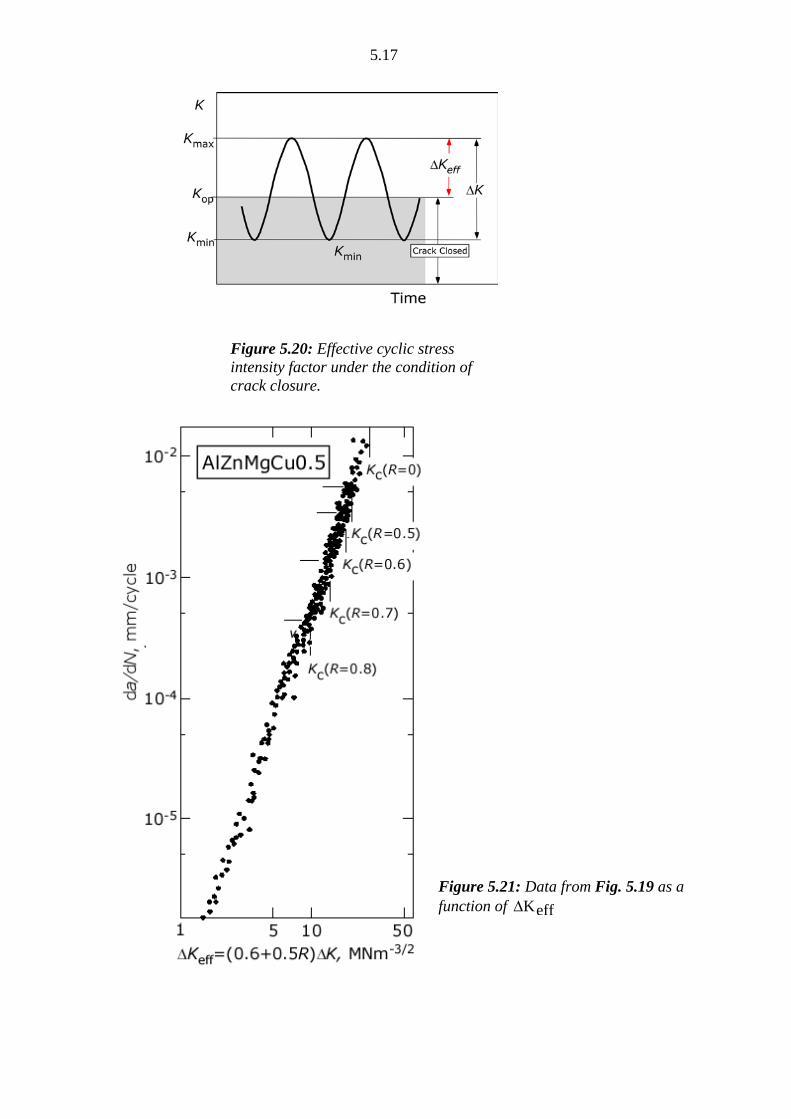
and hence no longer effective as a stress raiser. As a consequence, only a reduced cyclic stress intensity factor, effK∆ , given by K)bRa(effK ∆+=∆ (5.23) will contribute to crack propagation, Fig. 5.20. The application to the data shown in Fig. 5.19 setting a = 0.6 and b = 0.5 is demonstrated in Fig. 5.21. Above R equal to 0.4 to 0.6 the crack is fully open. The variation of thK∆ with R can be approximated by [5.16] 0R,thK)R1/()R1(thK =∆+−≅∆ (5.24)

Figure 5.19: Application of Eq.(5.21) to data of an aluminium alloy[5.14].

5.17

Figure 5.21: Data from Fig. 5.19 as a function of effK∆

Figure 5.20: Effective cyclic stress intensity factor under the condition of crack closure.

5.18

Three different mechanisms are proposed as origins of crack closure, which may occur individually or in combination [5.17, 5.18]:

1. Plasticity. Residual plastic deformations on the crack faces form a material wedge leading to contact of the crack faces at unloading.

2. Oxides. A material wedge may also develop as a consequence of oxidation processes due to reactions between the fresh material surfaces with the environment.

3. Roughness. A certain misfit of mating crack faces may occur due to a small mode II displacement and a pronounced crack deviation, thus leading to crack face contact upon unloading. These effects can be enhanced by designing specific microstructures whereby the crack propagation rate can be reduced [5.18].

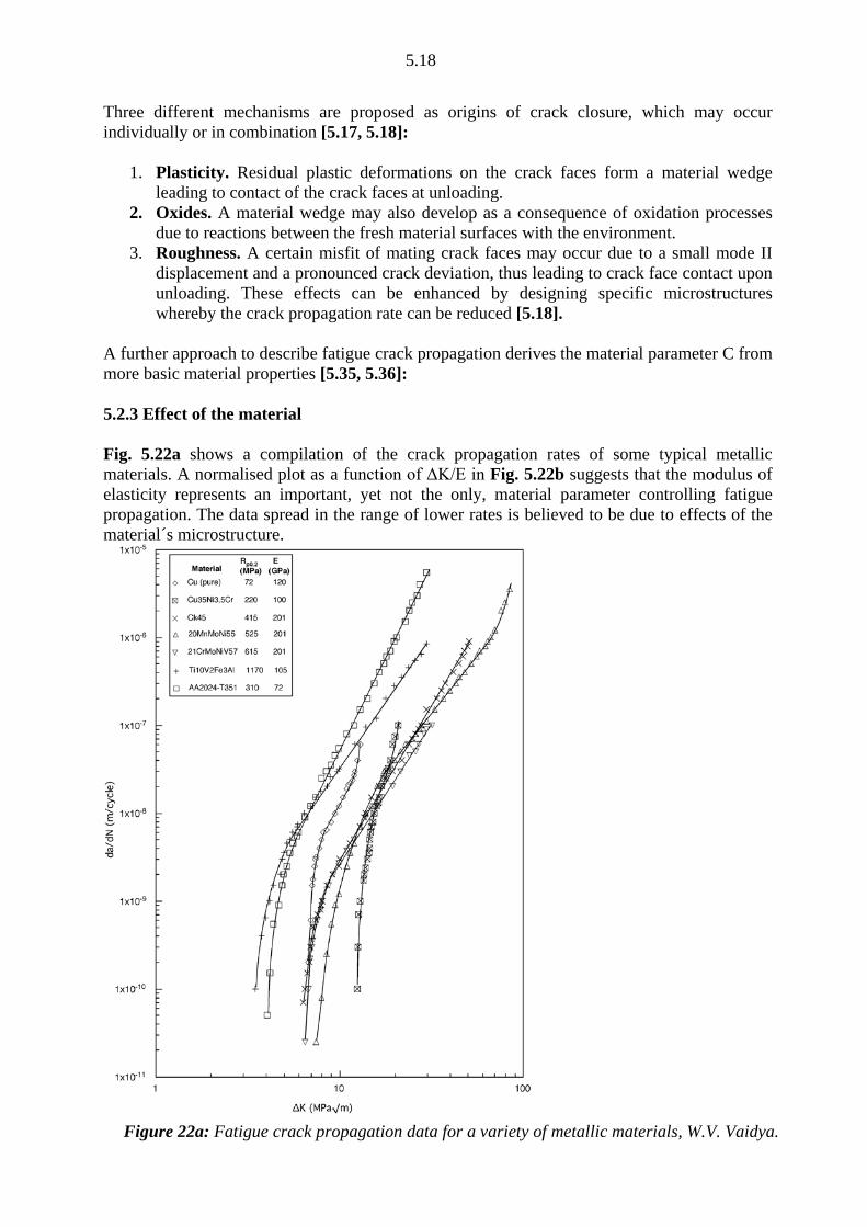
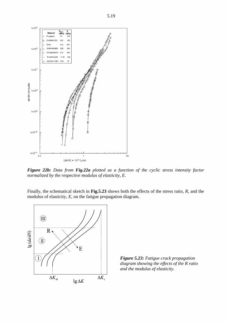
A further approach to describe fatigue crack propagation derives the material parameter C from more basic material properties [5.35, 5.36]: 5.2.3 Effect of the material Fig. 5.22a shows a compilation of the crack propagation rates of some typical metallic materials. A normalised plot as a function of ΔK/E in Fig. 5.22b suggests that the modulus of elasticity represents an important, yet not the only, material parameter controlling fatigue propagation. The data spread in the range of lower rates is believed to be due to effects of the material´s microstructure.

Figure 22a: Fatigue crack propagation data for a variety of metallic materials, W.V. Vaidya.

5.19

Figure 22b: Data from Fig.22a plotted as a function of the cyclic stress intensity factor normalized by the respective modulus of elasticity, E. Finally, the schematical sketch in Fig.5.23 shows both the effects of the stress ratio, R, and the modulus of elasticity, E, on the fatigue propagation diagram.

Figure 5.23: Fatigue crack propagation diagram showing the effects of the R ratio and the modulus of elasticity.

5.20

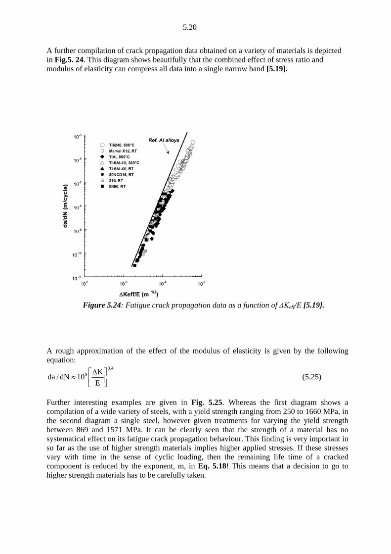
A further compilation of crack propagation data obtained on a variety of materials is depicted in Fig.5. 24. This diagram shows beautifully that the combined effect of stress ratio and modulus of elasticity can compress all data into a single narrow band [5.19].

A rough approximation of the effect of the modulus of elasticity is given by the following equation:

4.39

EK10dN/da

∆≈ (5.25)

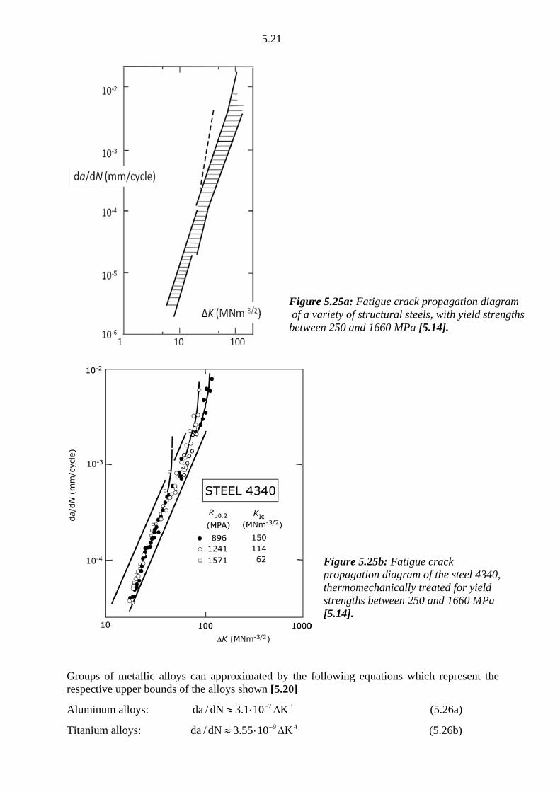
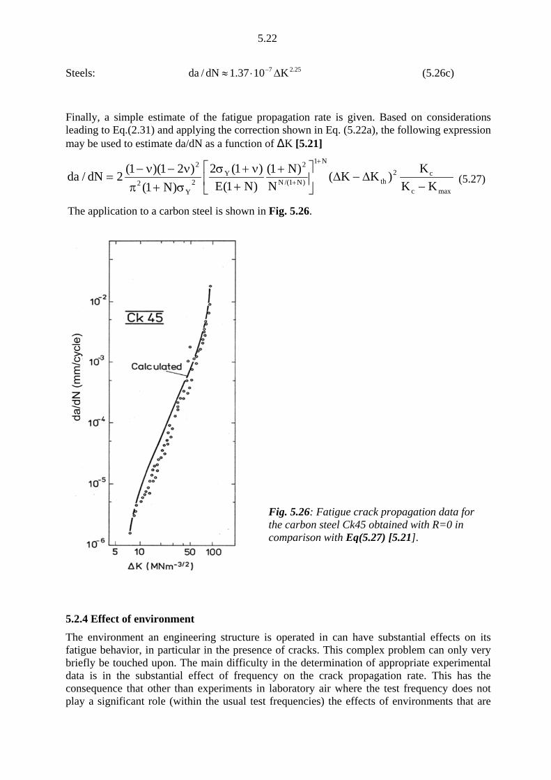
Further interesting examples are given in Fig. 5.25. Whereas the first diagram shows a compilation of a wide variety of steels, with a yield strength ranging from 250 to 1660 MPa, in the second diagram a single steel, however given treatments for varying the yield strength between 869 and 1571 MPa. It can be clearly seen that the strength of a material has no systematical effect on its fatigue crack propagation behaviour. This finding is very important in so far as the use of higher strength materials implies higher applied stresses. If these stresses vary with time in the sense of cyclic loading, then the remaining life time of a cracked component is reduced by the exponent, m, in Eq. 5.18! This means that a decision to go to higher strength materials has to be carefully taken.

Figure 5.24: Fatigue crack propagation data as a function of ΔKeff/E [5.19].

5.21

Groups of metallic alloys can approximated by the following equations which represent the respective upper bounds of the alloys shown [5.20]

Aluminum alloys: 37 K101.3dN/da ∆⋅≈ − (5.26a)

Titanium alloys: 49 K1055.3dN/da ∆⋅≈ − (5.26b)

Figure 5.25b: Fatigue crack propagation diagram of the steel 4340, thermomechanically treated for yield strengths between 250 and 1660 MPa [5.14].

Figure 5.25a: Fatigue crack propagation diagram of a variety of structural steels, with yield strengths between 250 and 1660 MPa [5.14].

5.22

Steels: 25.27 K1037.1dN/da ∆⋅≈ − (5.26c)

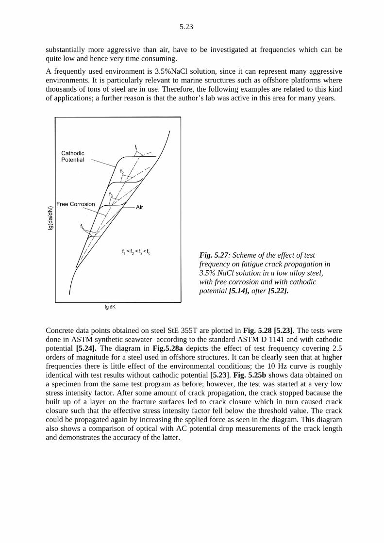
Finally, a simple estimate of the fatigue propagation rate is given. Based on considerations leading to Eq.(2.31) and applying the correction shown in Eq. (5.22a), the following expression may be used to estimate da/dN as a function of ΔK [5.21]

maxc

c2th

N1

)N1/(N

2Y

2Y

2

2

KKK)KK(

N)N1(

)N1(E)1(2

)N1()21)(1(2dN/da

−∆−∆

++

ν+σσ+πν−ν−

=+

+ (5.27)

5.2.4 Effect of environment The environment an engineering structure is operated in can have substantial effects on its fatigue behavior, in particular in the presence of cracks. This complex problem can only very briefly be touched upon. The main difficulty in the determination of appropriate experimental data is in the substantial effect of frequency on the crack propagation rate. This has the consequence that other than experiments in laboratory air where the test frequency does not play a significant role (within the usual test frequencies) the effects of environments that are

Fig. 5.26: Fatigue crack propagation data for the carbon steel Ck45 obtained with R=0 in comparison with Eq(5.27) [5.21].

The application to a carbon steel is shown in Fig. 5.26.

5.23

substantially more aggressive than air, have to be investigated at frequencies which can be quite low and hence very time consuming.

A frequently used environment is 3.5%NaCl solution, since it can represent many aggressive environments. It is particularly relevant to marine structures such as offshore platforms where thousands of tons of steel are in use. Therefore, the following examples are related to this kind of applications; a further reason is that the author’s lab was active in this area for many years.

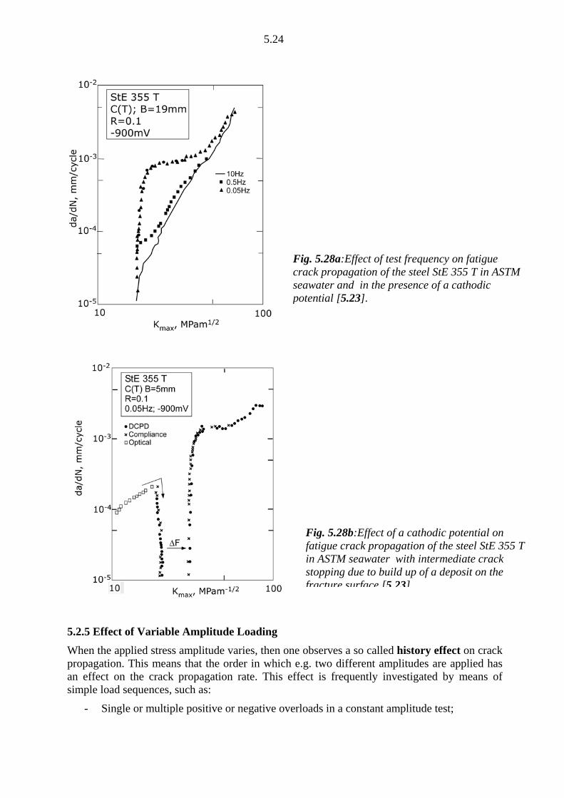
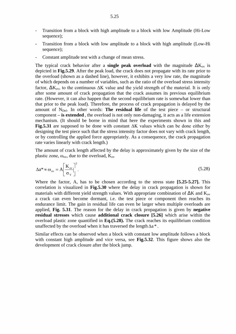
Concrete data points obtained on steel StE 355T are plotted in Fig. 5.28 [5.23]. The tests were done in ASTM synthetic seawater according to the standard ASTM D 1141 and with cathodic potential [5.24]. The diagram in Fig.5.28a depicts the effect of test frequency covering 2.5 orders of magnitude for a steel used in offshore structures. It can be clearly seen that at higher frequencies there is little effect of the environmental conditions; the 10 Hz curve is roughly identical with test results without cathodic potential [5.23]. Fig. 5.25b shows data obtained on a specimen from the same test program as before; however, the test was started at a very low stress intensity factor. After some amount of crack propagation, the crack stopped bacause the built up of a layer on the fracture surfaces led to crack closure which in turn caused crack closure such that the effective stress intensity factor fell below the threshold value. The crack could be propagated again by increasing the spplied force as seen in the diagram. This diagram also shows a comparison of optical with AC potential drop measurements of the crack length and demonstrates the accuracy of the latter.

Fig. 5.27: Scheme of the effect of test frequency on fatigue crack propagation in 3.5% NaCl solution in a low alloy steel, with free corrosion and with cathodic potential [5.14], after [5.22].

5.24

5.2.5 Effect of Variable Amplitude Loading When the applied stress amplitude varies, then one observes a so called history effect on crack propagation. This means that the order in which e.g. two different amplitudes are applied has an effect on the crack propagation rate. This effect is frequently investigated by means of simple load sequences, such as:

- Single or multiple positive or negative overloads in a constant amplitude test;

Fig. 5.28a:Effect of test frequency on fatigue crack propagation of the steel StE 355 T in ASTM seawater and in the presence of a cathodic potential [5.23].

Fig. 5.28b:Effect of a cathodic potential on fatigue crack propagation of the steel StE 355 T in ASTM seawater with intermediate crack stopping due to build up of a deposit on the fracture surface [5.23]

5.25

- Transition from a block with high amplitude to a block with low Amplitude (Hi-Low sequence);

- Transition from a block with low amplitude to a block with high amplitude (Low-Hi sequence);

- Constant amplitude test with a change of mean stress.

The typical crack behavior after a single peak overload with the magnitude ΔKov is depicted in Fig.5.29. After the peak load, the crack does not propagate with its rate prior to the overload (shown as a dashed line), however, it exhibits a very low rate, the magnitude of which depends on a number of variables, such as the ratio of the overload stress intensity factor, ΔKov, to the continuous ΔK value and the yield strength of the material. It is only after some amount of crack propagation that the crack assumes its previous equilibrium rate. (However, it can also happen that the second equilibrium rate is somewhat lower than that prior to the peak load). Therefore, the process of crack propagation is delayed by the amount of NDel. In other words: The residual life of the test piece – or structural component – is extended , the overload is not only non-damaging, it acts as a life extension mechanism. (It should be borne in mind that here the experiments shown in this and Fig.5.31 are supposed to be done with constant ΔK values which can be done either by designing the test piece such that the stress intensity factor does not vary with crack length, or by controlling the applied force appropriately. As a consequence, the crack propagation rate varies linearly with crack length.)

The amount of crack length affected by the delay is approximately given by the size of the plastic zone, ωov, due to the overload, Kov

2

Y

ovov

KA*a

σ

=ω≈∆ , (5.28)

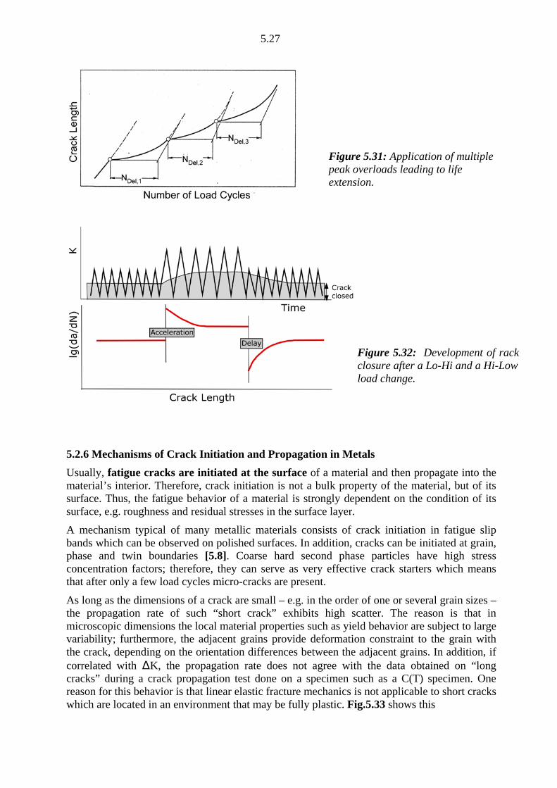
Where the factor, A, has to be chosen according to the stress state [5.25-5.27]. This correlation is visualized in Fig.5.30 where the delay in crack propagation is shown for materials with different yield strength values. With appropriate combination of ΔK and Kov a crack can even become dormant, i.e. the test piece or component then reaches its endurance limit. The gain in residual life can even be larger when multiple overloads are applied, Fig. 5.31. The reason for the delay in crack propagation is given by negative residual stresses which cause additional crack closure [5.26] which arise within the overload plastic zone quantified in Eq.(5.28). The crack reaches its equilibrium condition unaffected by the overload when it has traversed the length *a∆ .

Similar effects can be observed when a block with constant low amplitude follows a block with constant high amplitude and vice versa, see Fig.5.32. This figure shows also the development of crack closure after the block jump.

5.26

Figure 5.29: Effect of a peak overload on successive crack propagation. (a) Load under constant amplitude with single peak overload; (b) Development of crack length after overload; (c) Development of crack propagation rate after overload.

Figure 5.30: Effect of yield strength and stress ratio on crack propagation delay [5.28].

5.27

5.2.6 Mechanisms of Crack Initiation and Propagation in Metals Usually, fatigue cracks are initiated at the surface of a material and then propagate into the material’s interior. Therefore, crack initiation is not a bulk property of the material, but of its surface. Thus, the fatigue behavior of a material is strongly dependent on the condition of its surface, e.g. roughness and residual stresses in the surface layer.

A mechanism typical of many metallic materials consists of crack initiation in fatigue slip bands which can be observed on polished surfaces. In addition, cracks can be initiated at grain, phase and twin boundaries [5.8]. Coarse hard second phase particles have high stress concentration factors; therefore, they can serve as very effective crack starters which means that after only a few load cycles micro-cracks are present.

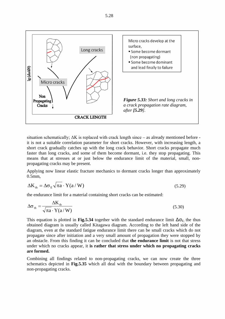
As long as the dimensions of a crack are small – e.g. in the order of one or several grain sizes – the propagation rate of such “short crack” exhibits high scatter. The reason is that in microscopic dimensions the local material properties such as yield behavior are subject to large variability; furthermore, the adjacent grains provide deformation constraint to the grain with the crack, depending on the orientation differences between the adjacent grains. In addition, if correlated with ΔK, the propagation rate does not agree with the data obtained on “long cracks” during a crack propagation test done on a specimen such as a C(T) specimen. One reason for this behavior is that linear elastic fracture mechanics is not applicable to short cracks which are located in an environment that may be fully plastic. Fig.5.33 shows this

Figure 5.32: Development of rack closure after a Lo-Hi and a Hi-Low load change.

Figure 5.31: Application of multiple peak overloads leading to life extension.

5.28

situation schematically; ΔK is replaced with crack length since – as already mentioned before - it is not a suitable correlation parameter for short cracks. However, with increasing length, a short crack gradually catches up with the long crack behavior. Short cracks propagate much faster than long cracks, and some of them become dormant, i.e. they stop propagating. This means that at stresses at or just below the endurance limit of the material, small, non-propagating cracks may be present.

Applying now linear elastic fracture mechanics to dormant cracks longer than approximately 0.5mm,

)W/a(YaK Eth ⋅πσ∆=∆ (5.29)

the endurance limit for a material containing short cracks can be estimated:

)W/a(YaK th

th⋅π∆

=σ∆ (5.30)

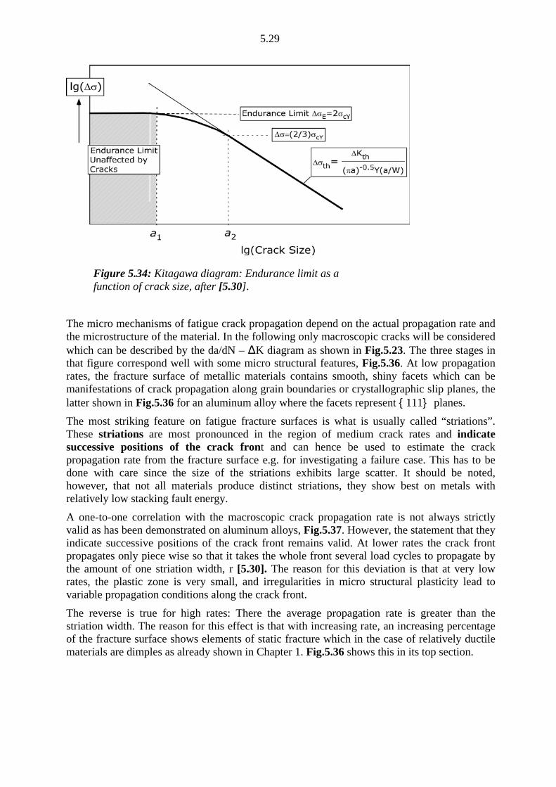
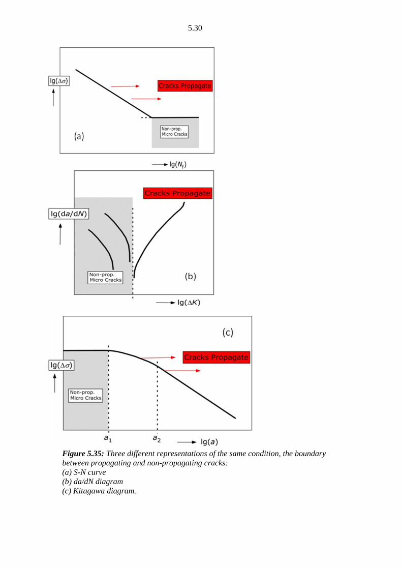
This equation is plotted in Fig.5.34 together with the standard endurance limit ΔσE; the thus obtained diagram is usually called Kitagawa diagram. According to the left hand side of the diagram, even at the standard fatigue endurance limit there can be small cracks which do not propagate since after initiation and a very small amount of propagation they were stopped by an obstacle. From this finding it can be concluded that the endurance limit is not that stress under which no cracks appear, it is rather that stress under which no propagating cracks are formed. Combining all findings related to non-propagating cracks, we can now create the three schematics depicted in Fig.5.35 which all deal with the boundary between propagating and non-propagating cracks.

Figure 5.33: Short and long cracks in a crack propagation rate diagram, after [5.29].

5.29

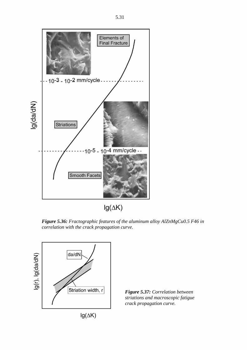
The micro mechanisms of fatigue crack propagation depend on the actual propagation rate and the microstructure of the material. In the following only macroscopic cracks will be considered which can be described by the da/dN – ΔK diagram as shown in Fig.5.23. The three stages in that figure correspond well with some micro structural features, Fig.5.36. At low propagation rates, the fracture surface of metallic materials contains smooth, shiny facets which can be manifestations of crack propagation along grain boundaries or crystallographic slip planes, the latter shown in Fig.5.36 for an aluminum alloy where the facets represent {111} planes.

The most striking feature on fatigue fracture surfaces is what is usually called “striations”. These striations are most pronounced in the region of medium crack rates and indicate successive positions of the crack front and can hence be used to estimate the crack propagation rate from the fracture surface e.g. for investigating a failure case. This has to be done with care since the size of the striations exhibits large scatter. It should be noted, however, that not all materials produce distinct striations, they show best on metals with relatively low stacking fault energy.

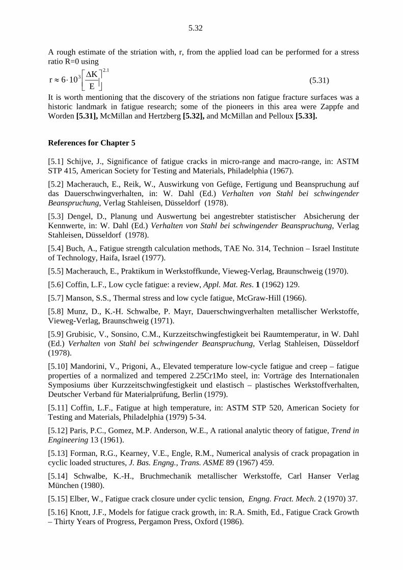
A one-to-one correlation with the macroscopic crack propagation rate is not always strictly valid as has been demonstrated on aluminum alloys, Fig.5.37. However, the statement that they indicate successive positions of the crack front remains valid. At lower rates the crack front propagates only piece wise so that it takes the whole front several load cycles to propagate by the amount of one striation width, r [5.30]. The reason for this deviation is that at very low rates, the plastic zone is very small, and irregularities in micro structural plasticity lead to variable propagation conditions along the crack front.

The reverse is true for high rates: There the average propagation rate is greater than the striation width. The reason for this effect is that with increasing rate, an increasing percentage of the fracture surface shows elements of static fracture which in the case of relatively ductile materials are dimples as already shown in Chapter 1. Fig.5.36 shows this in its top section.

Figure 5.34: Kitagawa diagram: Endurance limit as a function of crack size, after [5.30].

5.30

Figure 5.35: Three different representations of the same condition, the boundary between propagating and non-propagating cracks: (a) S-N curve (b) da/dN diagram (c) Kitagawa diagram.

5.31

Figure 5.36: Fractographic features of the aluminum alloy AlZnMgCu0.5 F46 in correlation with the crack propagation curve.

Figure 5.37: Correlation between striations and macroscopic fatigue crack propagation curve.

5.32

A rough estimate of the striation with, r, from the applied load can be performed for a stress ratio R=0 using

1.23

EK106r

∆⋅≈ (5.31)

It is worth mentioning that the discovery of the striations non fatigue fracture surfaces was a historic landmark in fatigue research; some of the pioneers in this area were Zappfe and Worden [5.31], McMillan and Hertzberg [5.32], and McMillan and Pelloux [5.33].

References for Chapter 5 [5.1] Schijve, J., Significance of fatigue cracks in micro-range and macro-range, in: ASTM STP 415, American Society for Testing and Materials, Philadelphia (1967).

[5.2] Macherauch, E., Reik, W., Auswirkung von Gefüge, Fertigung und Beanspruchung auf das Dauerschwingverhalten, in: W. Dahl (Ed.) Verhalten von Stahl bei schwingender Beanspruchung, Verlag Stahleisen, Düsseldorf (1978).

[5.3] Dengel, D., Planung und Auswertung bei angestrebter statistischer Absicherung der Kennwerte, in: W. Dahl (Ed.) Verhalten von Stahl bei schwingender Beanspruchung, Verlag Stahleisen, Düsseldorf (1978).

[5.4] Buch, A., Fatigue strength calculation methods, TAE No. 314, Technion – Israel Institute of Technology, Haifa, Israel (1977).

[5.5] Macherauch, E., Praktikum in Werkstoffkunde, Vieweg-Verlag, Braunschweig (1970).

[5.6] Coffin, L.F., Low cycle fatigue: a review, Appl. Mat. Res. 1 (1962) 129.

[5.7] Manson, S.S., Thermal stress and low cycle fatigue, McGraw-Hill (1966).

[5.8] Munz, D., K.-H. Schwalbe, P. Mayr, Dauerschwingverhalten metallischer Werkstoffe, Vieweg-Verlag, Braunschweig (1971).

[5.9] Grubisic, V., Sonsino, C.M., Kurzzeitschwingfestigkeit bei Raumtemperatur, in W. Dahl (Ed.) Verhalten von Stahl bei schwingender Beanspruchung, Verlag Stahleisen, Düsseldorf (1978).

[5.10] Mandorini, V., Prigoni, A., Elevated temperature low-cycle fatigue and creep – fatigue properties of a normalized and tempered 2.25Cr1Mo steel, in: Vorträge des Internationalen Symposiums über Kurzzeitschwingfestigkeit und elastisch – plastisches Werkstoffverhalten, Deutscher Verband für Materialprüfung, Berlin (1979).

[5.11] Coffin, L.F., Fatigue at high temperature, in: ASTM STP 520, American Society for Testing and Materials, Philadelphia (1979) 5-34.

[5.12] Paris, P.C., Gomez, M.P. Anderson, W.E., A rational analytic theory of fatigue, Trend in Engineering 13 (1961).

[5.13] Forman, R.G., Kearney, V.E., Engle, R.M., Numerical analysis of crack propagation in cyclic loaded structures, J. Bas. Engng., Trans. ASME 89 (1967) 459.

[5.14] Schwalbe, K.-H., Bruchmechanik metallischer Werkstoffe, Carl Hanser Verlag München (1980).

[5.15] Elber, W., Fatigue crack closure under cyclic tension, Engng. Fract. Mech. 2 (1970) 37.

[5.16] Knott, J.F., Models for fatigue crack growth, in: R.A. Smith, Ed., Fatigue Crack Growth – Thirty Years of Progress, Pergamon Press, Oxford (1986).

5.33

[5.17] Fleck, N.A., Fatigue crack growth – the complications, in: R.A. Smith, Ed., Fatigue Crack Growth – Thirty Years of Progress, Pergamon Press, Oxford (1986).

[5.18] Shang, J.K., Tzou, J.L., Ritchie, R.O., Role of crack tip shielding in the initiation and growth of long and small fatigue cracks in composite microstructures, Met. Trans. A, 18A (1987) 1613.

[5.19] Petit, J., European Conference on Fracture 18, Dresden, 30 August – 3 September 2010.

[5.20] Clark, W.G., Jr., How fatigue crack initiation and growth properties affect material selection and design criteria, Metals Engineering Quarterly (1974) 16.

[5.21] Schwalbe, K.-H., Mechanik und Mechanismen des stabilen Risswachstums in metallischen Werkstoffen, Thesis for Habilitation, Ruhr University Bochum, Bochum (1977).

[5.22] Vosikovsky, O., Fatigue-crack growth in an X-65 line-pipe steel at low frequencies in aqueous environments, Closed Loop (1969) 3.

[5.23] Wellenkötter, B., Horstmann, M., Schwalbe, K.-H., Schwingungsrisskorrosion von Stahl in synthetischem Meerwasser (ASTM-Standard) ohne und mit kathodischer Polarisation, Proceedings of the 20th Meeting of the German Association of Materials Research and Materials Testing (DVM), Berlin (1988) 407-414.

[5.24] ASTM D 1141, Annual Book of ASTM Standards, Vol.11.02, American Society of Testing and Materials, Philadelphia (1986) 536.

[5.25] Trebules, V.W., Jr., Roberts, R., Hertzberg, R.W., Effect of multiple overloads on fatigue crack propagation in 2024-T3 aluminum alloy, In: ASTM STP 536 (1973).

[5.26] Lankford, J., Jr., Davidson, D.L., Fatigue crack tip plasticity associated with overloads and subsequent cycling, J. Engng. Materials and Technology (Trans. ASME) 98 (1976) 17.

[5.27] Mills, W.J., Load interaction effects on fatigue crack growth in 2014-T3 aluminum and A514F steel alloys, PhD. Thesis Dept. of Metallurgy and Materials Science, Lehigh University (1975).

[5.28] Njus, G.O., Stephens, R.I., The influence of yield strength and negative stress ratio on fatigue crack growth delay in 4140 steel, Int. Journ. of Fracture, ??? [5.29] Miller, K.J., de los Rios, E.R. (Eds.) The Behaviour of Short Fatigue Cracks, Mechanical Engineering Publications Ltd., London (1986).

[5.30] Schwalbe, K.-H. Bruchflächenuntersuchungen bei derAusbreitung von Ermüdungsrissen in AlZnMgCu 0,5 F46, Z. Metallkunde 66 (1975) 408-416. (English translation: Fracture surface observations of fatigue crack growth in AlZnMgCu 0,5 F46, Report 1878,, Royal Aircraft Establishment, Farnborough, U.K. (1976).

[5.31] Zappfe, C.A., Worden, C.O., Fractographic registrations of fatigue, Trans.ASM 43 (1951) 958.

[5.32] McMillan, J.C., Hertzberg, R.W., Application of electron fractography to fatigue studies, in: ASTM STP 436 (1968).

[5.33] McMillan, J.C., Pelloux, R.M.N., Fatigue crack propagation under program and random loads, in: ASTM STP 436 (1968).

5.34

5.35