1

CHAPTER 5

OPTIMIZATION TECHNIQUES FOR GRAPH

PARTITIONING

5.1 Introduction

Most real life problems have several solutions and occasionally an infinite

number of solutions may be possible. If the problem at hand admits more than

one solution, optimization can be achieved by finding the best solution of the

problem in terms of some performance criterion. The graph partitioning problem

(GPP) deals with the partition of vertices in a certain number of blocks in such a

way that the edge cut is minimized. While partitioning graph, a balance

constraint that all blocks must be of the same weight should also be maintained.

Thus, optimization techniques are considered necessary for best partition with

optimized cut value. This chapter focuses on local search optimization

techniques like Simulated Annealing, Genetic Algorithm, Tabu Search, Random

Walk, Neighborhood Search, Swarm intelligence based Ant Colony

Optimization, and Particle Swarm Optimization. These optimization techniques

are characterized by the use of local search method, recursively applied to the

solution of the problem.

5.2 Optimization Techniques

Multi-objective optimization (MOO) or vector optimization is the process of

optimizing systematically and simultaneously a collection of objective functions

[127]. Graph partitioning is a NP-hard problem with multiple conflicting

objectives such as the inter-partition relationship should be minimized while

maximizing the intra-partition relationship as well as balance constraint that all

2

blocks must be of the same weight should also be maintained. Hence graph

partitioning is a multi-objective optimization problem. The optimization

techniques used in graph partitioning are described below:

5.2.1 Simulated Annealing

Simulated Annealing (SA) is a standard probabilistic metaheuristic for the global

optimization problem of a given function in a large search space for locating a

good approximation to the global optimum. It is frequently used when the

search space is discrete. The main advantage of SA is its capability of moving to

states of higher energies. Simulated Annealing can be effectively used in graph

partitioning to find a balanced partition which can minimize edge cut.

Kirkpatrick et al. [128] introduced simulated annealing to solve combinatorial

optimization problem. Simulated annealing is tried and tested technique, which

can be simply located in space, easy to locate in place and which often generates

motivating results in short programming time. Hence it is an interesting method

for implementation before the use of sophisticated methods. In GPP simulated

annealing is used as direct graph partitioning tool [129, 130] also in multilevel

partitioning it is used as partition refinement tool [131, 132].

5.2.1.1 Principle and Model of Simulated Annealing

Simulated annealing methodology is inspired by the physical process of

annealing in metallurgy. In annealing, a solid is heated to a high temperature

and gradually cooled down crystallization. At high temperatures, the atoms

move randomly with high kinetic energy, but during the cooling process, they

have a tendency to align themselves to the minimum energy state [133]. The

algorithm of simulated annealing is based on two loops called as internal loop

and external loop. Iterations in an internal loop continues still the system

becomes stable. Whereas as external loop reduces the temperature to simulate

annealing of stable systems. The internal loop generates new state by basic

alterations in previous one and then applies it to the Metropolis acceptance rule.

3

The best state generated by the algorithm is preserved and updated successively

by internal loop.

The process flow of simulated annealing is as shown in Fig. 5.1. Point E’ is

generated within a state space from the existing point E at each step in the

algorithm. Point E’ accepted unconditionally if it has a lower cost function than

E. But if it has a higher cost, then it is accepted using the metropolis criterion

described below. This acceptance probability is proportional to the temperature

T of the annealing process, which is lowered steadily as the algorithm proceeds.

The symbol description for Simulated Annealing is presented in Table 5.1.

Fig. 5.1: Process Flow for Simulated Annealing

No

No

Start with E, Temperature T

Find best E’ N(E)

Is f (E’) <f (E)DecreaseT

Metropolisacceptance rule

satisfied

E = E’

Internal loopCompleted?

Output E* = Point with best evaluation so far

Yes

No

Yes

Yes

Stop

Yes

No

4

Symbol Description

E State Space

E’ Optimized State Space

N(E) Number of State Space

T Temperature

Table 5.1: Symbol Description for Simulated Annealing

For E’ belonging to state space, the probability that E’ gets selected is given by

the relation: → = 1, ( )(5.1)

If T is high initially, then high probability of making uphill moves exists. It

allows the search to fully explore the state space. Simulated Annealing will

converge asymptotically to global optimum under two conditions [134]:

Homogeneous Condition: If T is lowered to 0 in anyway, while the length

of the homogeneous sequence formed by the accepted points at each

temperature is increased to an infinite length.

Inhomogeneous Condition: Irrespective of the length of these isothermal

chains, the cooling schedule is chosen so that T approaches to 0 at a

logarithmically slow rate.

In practice neither of this is possible in infinite implementations, hence

polynomial time approximations are used. The quality of results and the rate of

convergence are affected by the choice of cooling schedule and the length of

chain at each temperature. The SA program is ended if an acceptable solution is

originated or if a designated final temperature is reached. Simulated Annealing

is successful in a wide range of NP-hard optimization problems.

5

5.2.1.2 Adaptation of Simulated Annealing for Graph Partitioning

Johnson et al [135] adapted simulated annealing for graph bipartitioning. Since

simulated annealing based on the notion of moving from one state to the

neighboring state, in this context two partitions are neighbors if by moving single

vertex from one part to the other part we can go from one partition to the other

partition. Cost function for the bipartition of graph = ( , )with two

neighboring partitions for ∈ , = ( , ) and = ( − { }, ∪ { })used in

[13] is:

( ) = ( ) + (| | − | |) (5.2)

where is constant. Authors have shown that this cost function bisects the

graph, but balance constraint is compromised. Penalty function is the second

part of cost function which allows escaping from local minimum by passing

through the unauthorized state. For proper choice of , penalty function forces

the balanced partition. But the disadvantage is that it involves an inability of

returning to an unacceptable state for larger graphs. Heuristic technique is used

to improve the balance constraint. An adaptation of simulated annealing gives

results similar to KL algorithm discussed in section 2.3.2 for smaller graphs(100 ≤ | | ≤ 1000), but execution time is longer.

Simulated annealing to graph bipartitioning is extended to k – partitioning of

weighted graphs by C. Bichot [136]. Cost function for the k - partitioning of graph= ( , ) with partition = { , ,… , } is:( ) = ( ) + ∑ ( )∈{ , ,…, } − ∑ ( )∈{ , ,…, } (5.3)

In case of k – partitioning, two partitions are neighbors if by moving single vertex

from one part to the other part we can go from one partition to the other k – 1

partitions. As a result neighborhood is very large, hence adaptation to k –

partitioning is minimal.

6

Adaptation of simulated annealing to optimization of GPP is relatively easy to

implement with biggest advantage of its flexibility to the acceptance of different

objective functions and constraints of partitioning [136]. But these adaptations

are very slow as compared with other methods. SA can be used constructively

for smaller graphs with non - traditional objective functions.

5.2.2 Genetic Algorithm (GA)

Genetic Algorithms (GAs) are robust ways which can be used in search and

optimization issues based on Darvin’s principle of natural selection. Genetic

Algorithm is one of the best optimization algorithms having great potential to

deal with various problem areas like graph partitioning, image processing, and

routing issues. The idea behind GA is that the combination of exceptional

characteristics from different ancestors generates the better and optimized off

springs that is having an improved fitness function than the ancestors.

Implementing this mechanism iteratively the off springs gets more optimized,

resulting into higher sustainability in the environment. The parameter set of the

optimization problem is required to be coded as a finite-length string or

chromosome. Population in GA is a collection of strings or a chromosome [137].

Adaptation of chromosome to the environment is evaluated using objective

function. Hence the objective function in GA is called as fitness function. Basic

GA is composed of three operators:

Selection – Forms population by selecting parents to reproduce

chromosome at first stage, then the chromosomes generated in first stage

are selected to generate population for the next stage.

Crossover - This operator requires two parents to generate several

offsprings by combination of genes.

Mutation– This operator is created by constrained random modifications

of one or many genes of chromosomes.

7

Mutation is used to explore the solution space and crossover to reach to the local

optima [138]. In GA population evolves iteratively, it starts with a randomly

generate initial population; a new population is generated from the existing

population by selection, crossover, and mutation. Fitness function in GPP is the

inverse of the objective function of minimizing edge cut. Several GA adaptations

have been proposed to solve graph partitioning optimization problem [139 -

141]. In GPP number of vertices of graph represents size of chromosome,

crossover operators are cut vertices and mutation operators are vertices

involved in exchanges between parts.

5.2.2.1 Principle and Model of Genetic Algorithm

Cross breeding with alternative chromosome within the population occurs by

giving opportunities to highly appropriate chromosomes. This breeding

generates chromosome as offspring and this offspring shares some characteristics

taken from every parent. By favoring the mating of the additional appropriate

chromosome, the foremost promising areas of the search house are explored.

Convergence to an optimal solution of the population of chromosomes depends

on the structure of Genetic Algorithm.

The process flow of Genetic Algorithm is shown as in Fig. 5.2. Randomly select

an initial population P of n chromosomes. At every iteration; a new population P’

is generated by choosing two parents from P with the probability of selection

proportional to their fitness. Generate new offsprings by crossover from selected

parents with probability Pc, and then by random mutation recombine these

chromosomes with some probability Pm(0.001 ≤ ≤ 0.01). Newly generated

population replaces the existing population.

8

Yes

Initialize population P

Evaluate P

Chromosome Selection by best fit

Crossover with Probability Pc

Mutation with probability Pm

Output: Best adapted chromosome

TerminateNo

Yes

P’ generated

P = P’

No

Fig. 5.2: Process Flow for Genetic Algorithm

Termination criteria can be either the number of generations or the best fit for

chromosomes or even time elapsed. For specific applications, redefine or extend

crossover and mutation operators and to speed up the convergence initiate a

local search at the end of each generation. Depending on the choice of

implementation techniques, variations in encoding of solution space into

9

chromosomes, the size of population, mutation and crossover rate may be

observed. Genetic algorithms are better known in a variety of applications.

5.2.2.2 Adaptation of Genetic Algorithm for Graph Partitioning

Bui and Moon [138] exploits the potential of genetic algorithm to solve graph

partitioning problem. GPP studied in [139] is a graph bisection problem with

minimized cut and balanced bisection using Genetic Bisection Algorithm (GBA).

The GBA carries a single mutation and crossover per iteration, which decreases

the number of parameters in genetic algorithm by 2. Preprocessing step of GBA

modifies numbering of vertices in the initial graph G and new graph G ’is

generated which is reference graph for the remaining algorithm. At each

iteration, two parents are selected, then from these parents crossover operator

generates unique offspring and at the end mutation is applied to offspring.

Swapping depends on the quality of offspring generated; if the cut is comparable

to its parents then the most related parent is replaced by offspring. Otherwise,

least efficient chromosome of the population is replaced. The process continues

still 80% of the chromosomes have same cut value. Fitness function used in GBA

is:

( ) = ( )∈ − ( ) + ( ) − ( )∈∈ (5.4)

Partitions determined by GBA in case of ordinary graphs are of better quality but

it is multiple times slower than SCOTCH. M. Cross et al. [140] proposed use of GA

using multilevel method for k partitioning of the graph. They proposed Jostle

Evolutionary [JE] adaptation of hybrid multilevel GA for optimization of GPP. It

starts by creating 50 chromosomes randomly with limitation of maximum 1000

iterations. Each of 50 chromosomes generates offsprings using crossover and

10

mutation operator. The evaluation strategy replacement operator chooses the

new population for JE after offspring generation. Fitness function for this

algorithm is:

( ) = − ( ) ∗ ( ) , ∈ (5.5)Computation time of JE is several weeks for larger graphs.

However, it gives the best solution for graph partitioning, but it is really not

computationally efficient [141].

5.2.3 Tabu Search

Tabu search is a local heuristic method based on neighborhood initially proposed

by Glover and Laguna [142]. It explores the solution space by constantly

replacing recent solution with best non visited neighboring solution, new

solution may be less efficient. A fundamental concept in tabu search is that the

intelligent search must be based on learning; the usage of flexible memory

explores beyond optimality and exploits the earlier state of the search to

influence its future states [143]. Tabu lists are introduced to avoid cycling of

recently visited solutions and optimality crossing. In graph partitioning tabu

search algorithm utilizes two neighborhood relations S1 and S2 based on two

different move operators. These operators exchange vertices between subsets of

partition. Tabu search improves the number of current best partitions.

5.2.3.1 Principle and Flow of Tabu Search

Tabu search algorithm follows the search whenever a local optimum is

encountered by permitting non-improving moves; cycling back to earlier visited

solutions is prevented by the exploitation of memories, called the tabu list which

11

reports the recent history of the search. Tabus are one of the distinctive elements

of tabu search when compared with hill climbing methods.

The process flow of Tabu Search is as shown in Fig. 5.3. Tabu search begins

iteratively with local or neighborhood search from one solution to another still

selected termination criteria satisfied. Symbol description of Tabu Search is given

in table 5.2.

Symbol Description

Current solution

Best known solution( ) Value of s( ) Neighborhood of s′( ) Admissible subset of ( )T Tabu list

Table 5.2: Symbol Description for Tabu Search

Each solution s has neighborhood ( )∁ and solution ∈ ( ) is generated

from s by move. Objective function for tabu search is to minimize ( ). Tabu

search method permits moves which improve the current objective function

value and ends when no improving solution can be established. The algorithm

starts by selection of ∈ , then find ∈ ( ) such that ( ) < ( ). If no such

found then is the local optimum and algorithm stops. Otherwise designate

to new and repeat the process.

12

Find best s’ N(s)

No Yes

S = S’

No

Fig. 5.3: Process Flow of Tabu Search

No

Start with s, Tabu list T

Decrease T

Does s’ TUpdate T Aspiration

criterion satisfied

Terminate

Output s* = Point with best evaluation so far

Yes

Yes

13

5.2.3.2 Adaptation of Tabu Search for Graph Partitioning

Roland E. et al. [144] introduced an adaptation of tabu search algorithm for graph

partitioning. In this method all vertices having same gain are placed in partition

P ranked as g. Then find a nonempty partition with the highest rank, it yields

vertex with maximum gain. After each move, partition structure is updated by

computing gains of selected vertex and its neighbors then transfer to the

appropriate partition. Results yield by this algorithm are compared with a KL –

refinement algorithm and simulated annealing, gives motivating results for 149

graphs. But unfortunately works in smaller graphs with 10 to 500 vertices.

Multilevel algorithm proposed in [145] uses tabu search during partitioning and

refinement process. In this method modifications are suggested in the traditional

version of the KL/FM algorithm based on moving a vertex only once per round,

specific type of moves (u, block) are expelled only for few iterations. Number of

iterations for which move (v, block) is excluded depends on function f and current

iteration. Non excluded vertex with highest gain is always moved. If the vertex

is in block , then the move (v, ) to the block yielding the highest gain is

excluded for f(i) iterations means vertex cannot be placed back to the block for

f(i) iterations [61, 62] Advanced local search k – way algorithm is based on tabu

search, which has been applied to graph partitioning problem [63, 64].

In this algorithm, k has no influence on the performance in terms of computation

time. However, as k increases it requires larger memory. Results generated in a

short running time are far better than METIS and CHACO. For the prolonged

running time from one minute to one hour, the algorithm is converged towards

balancing which is far better than the methods having run time in weeks.

5.2.4 Random Walks (RWs)

Random walk (RWs) was originally introduced by Karl Pearson. A random walk

is mathematical formalization a path which consists of random steps in

14

succession. Random walk serves as a fundamental model for recording stochastic

activities which explains the observed behavior of the processes. Generally

random walks assumed as Markov Chains [146]. For different variations of RWs

in graph partitioning problem concepts like local search algorithm or path

determining strategy are also used. A random walk is an iterative process which

can be repeated arbitrary number of times starts with vertex v and then

randomly selects the next vertex to visit from the set of neighbors considering

transition probabilities. Diffusion is and iterative natural process in which

splittable entities between neighboring vertices are exchanged still all vertices

has same quantity. Diffusion is nothing but special random walk and hence both

can be used for identifying dense graph regions. This method is used in graph

clustering but balance constraint is neglected [147].

5.2.4.1 Principle and Flow of Random Walk

In Random Walk, the next step is selected uniformly between the neighbors of

the vertex. A main weakness of RW is the existence of loops in the path while

travelling from the source to the destination vertex. To prevent loops, the

simplest method is to introduce memory in the RWs.

The process flow for Random Walk is as shown in Fig. 5.4. RW is based on the

neighborhood search techniques. At each step a node ∈ ( ) is generated from

the existing node v.

If the cost function ′ for ′is less than ( ), then the node ′ accepted and

the search proceeds by setting v = v’. But if ′ is greater than ( ), then the

point ′ is accepted with probability of accepting ascending moves. The

complete family of random walk can be generated by varying parameter

P(0 ≤ ≤ 1), from greedy search to purely random search.

15

Greedy search will result in the search converging to local minimum and hence a

small nonzero uphill probability will help in escaping such minima. But, if the

uphill probability is too high, the search becomes more random and the

performance may drop.

Symbol Description

V Search Space

v’ Optimized Search Space

f(v) Cost Function

N(v) Number of search space

P Path considering probability

R Random Factor

Table 5.3: Symbol Description for Random Walk

Fig. 5.4: Process Flow for Random Walk

No

Start with v, P

Select v’ N(v)

Is f(v’) <f(v) Is R < P

v =v’

Terminate

Output v* = Point with best evaluation so far

Yes

No

Yes

No

Generate R in

[0, 1]randomlyYes

16

5.2.4.2 Adaptation of Random Walk for Graph Partitioning:

Meyerhenke [148] proposed similarity measure based on diffusion resembles to

the spectral partitioning can be employed within Bubble framework, with the

advantages in partitioning quality. Balancing is enforces by combining with the

actual partitioning process in two different ways. First one is iterative in which

diffusion load in each block is multiplied by an appropriate scalar. If an

appropriate scalar cannot be determined, then the second way is adopted, in

which migrating flow is computed on the quotient graph of partition. To balance

the partition, flow value fij between blocks i and j indicates number of nodes to be

migrated. For the best solution to migration of nodes diffusive similarity values

calculated within the Bubble framework are used [149, 150]. Pellegrini combined

KL/FM with diffusion to speed up previous approaches of bipartitioning in tool

Scotch. These results are extended for k – way partitioning with added variations

within the tools DibaP and PDibaP. In collaboration with multilevel method

diffusive partition generates high quality solutions, particularly in terms of

communication volume and block shape. However, faster implementation of

diffusion with running time independent of k is still undetermined.

5.2.5 Fusion - Fission

The Fusion – Fission method is originated from the nuclear process. The Nuclear

process generates atoms with great internal cohesion which is same as matter

reforming in an optimization process. In the nature, iron is an atom with the

greatest cohesion, with 56 nucleons ranging from 2 to 235 for the other atom. If

the number of nucleons and sort of nucleons permits, then reorganization of

nucleons of atoms generates iron atom. Graph partitioning problem correlates

with nuclear process, in which objective is to find a low energy organization of

parts of the graph. The vertices of the graph are nucleons and parts are atoms. In

Fusion – Fission process, parts of the partition are successively split or merged.

17

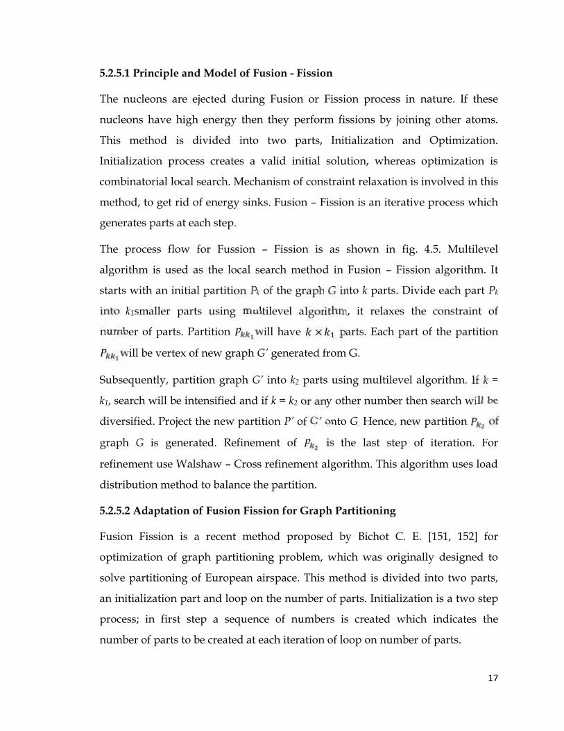
5.2.5.1 Principle and Model of Fusion - Fission

The nucleons are ejected during Fusion or Fission process in nature. If these

nucleons have high energy then they perform fissions by joining other atoms.

This method is divided into two parts, Initialization and Optimization.

Initialization process creates a valid initial solution, whereas optimization is

combinatorial local search. Mechanism of constraint relaxation is involved in this

method, to get rid of energy sinks. Fusion – Fission is an iterative process which

generates parts at each step.

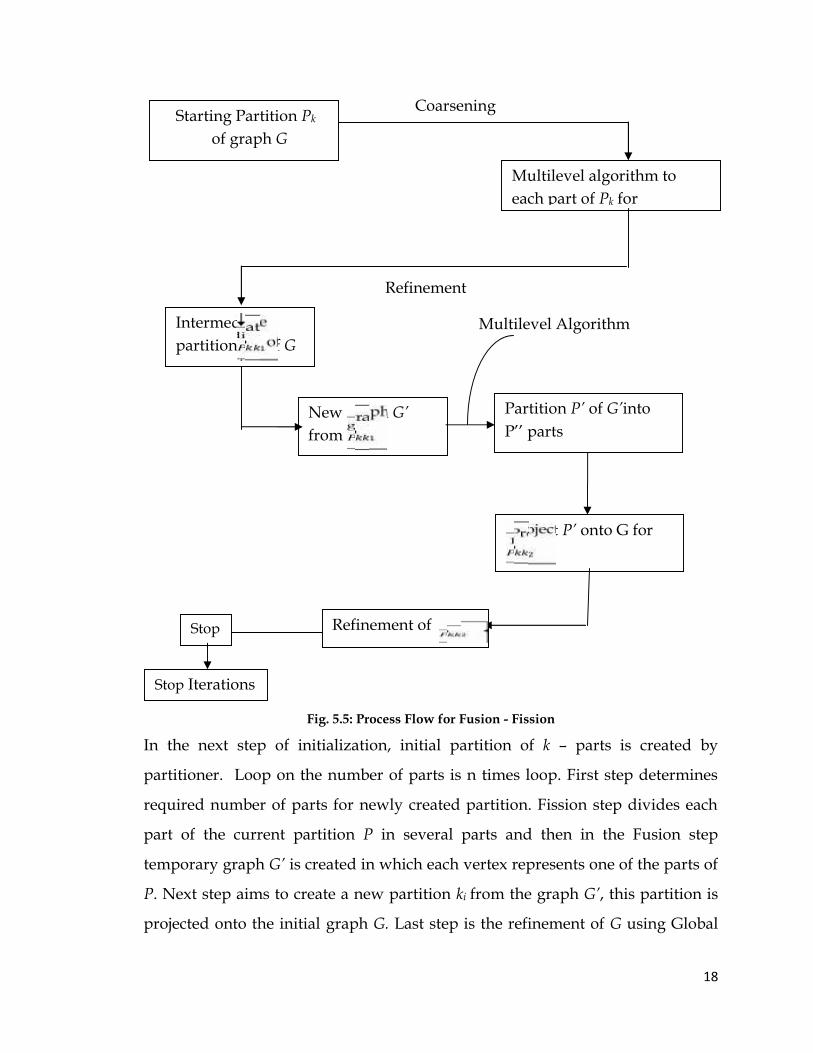
The process flow for Fussion – Fission is as shown in fig. 4.5. Multilevel

algorithm is used as the local search method in Fusion – Fission algorithm. It

starts with an initial partition Pk of the graph G into k parts. Divide each part Pk

into k1smaller parts using multilevel algorithm, it relaxes the constraint of

number of parts. Partition will have × parts. Each part of the partition

will be vertex of new graph G’ generated from G.

Subsequently, partition graph G’ into k2 parts using multilevel algorithm. If k =

k1, search will be intensified and if k = k2 or any other number then search will be

diversified. Project the new partition P’ of G’ onto G. Hence, new partition of

graph G is generated. Refinement of is the last step of iteration. For

refinement use Walshaw – Cross refinement algorithm. This algorithm uses load

distribution method to balance the partition.

5.2.5.2 Adaptation of Fusion Fission for Graph Partitioning

Fusion Fission is a recent method proposed by Bichot C. E. [151, 152] for

optimization of graph partitioning problem, which was originally designed to

solve partitioning of European airspace. This method is divided into two parts,

an initialization part and loop on the number of parts. Initialization is a two step

process; in first step a sequence of numbers is created which indicates the

number of parts to be created at each iteration of loop on number of parts.

18

Coarsening

Refinement

Multilevel Algorithm

Fig. 5.5: Process Flow for Fusion - Fission

In the next step of initialization, initial partition of k – parts is created by

partitioner. Loop on the number of parts is n times loop. First step determines

required number of parts for newly created partition. Fission step divides each

part of the current partition P in several parts and then in the Fusion step

temporary graph G’ is created in which each vertex represents one of the parts of

P. Next step aims to create a new partition ki from the graph G’, this partition is

projected onto the initial graph G. Last step is the refinement of G using Global

Starting Partition Pk

of graph G

Multilevel algorithm toeach part of Pk forpartitioning

Intermediatepartition of G

Partition P’ of G’intoP’’ parts

Project P’ onto G for

StopIterations

New graph G’from

Refinement of

Stop IterationsIIterations

19

Kernighan Lin Refinement (GKLR) algorithm. Fusion Fission method increases

the efficiency in comparison with the multilevel method, but its computation

time is very long.

5.3 Swarm IntelligenceA swarm is huge number of uniform, simple agents interacting locally among

themselves, and their environment to permit global interesting behavior to

appear without central control. Swarm-based algorithms are competent to

generate low cost, fast, and robust solutions to several complex problems.

These algorithms are known as nature–inspired or population-based

algorithms. [153, 154]. Swarm Intelligence (SI) can consequently be known as

comparatively new branch of Artificial Intelligence which is used to model

the collective behavior of social swarms in nature such as ant colonies, bird

flocks, and honey bees. Even though these insects or swarm individuals are

fairly simple with limited capabilities on their own, they interact jointly with

certain behavioral patterns for achieving tasks essential for their survival.

Swarm individuals or agents interact directly or indirectly. Waggle dance of

honey bees [155] is an example of direct interaction through visual or audio

contact. Indirect interaction occurs when one individual changes the

environment and the others respond to the new environment. Indirect

interaction is referred as stigmergy, which basically means communication

through the environment. Pheromone trails of ants which they deposit on their

way while searching for food sources is an example of indirect interaction . The

area of research presented in this depth paper focuses on Swarm Intelligence.

In next section, two of the most popular models of swarm intelligence inspired

by birds flocking behavior and ant’s stigmergic behavior are discussed in

detail.

20

5.3.1 Ant Colony Optimization (ACO)

Ant Colony Optimization is inspired by the foraging behavior of ants. At the core

of this behavior is the indirect communication between the ants with the help of

chemical pheromone trails, which enables them to find short paths between

their nest and food sources. Blum [156] exploited this characteristic of real ant

colonies in ACO algorithms to solve global optimization problems. Ant based

solution construction, pheromone update and daemon actions are the

algorithmic components involved in metaheuristic of ACO. Dorigo [157]

developed the first ant colony optimization algorithm and since then numerous

improvements of the ant system have been proposed. Ant colony optimization

algorithm (ACO) has strong robustness as well as good dispersed calculative

mechanism. ACO can be combined easily with other methods; it shows well

performance in resolving the complex optimization problem. The Travelling

Salesman Problem is selected as example to introduce the basic principle of ACO,

and now several improvement algorithms are developed for the problem of

ACO. This stochastic optimization method has been successfully applied in a

number of engineering as well as real world problems. ACO algorithm imitates

single ant colony which constructs solution in the form of parameters associated

with problem.

5.3.1.1 Principle and Model of ACO

Ant Colony Optimization (ACO) is a computational method which iteratively

optimizes a problem to pheromone with regard to a given transition probability.

ACO optimizes a problem by having a updated pheromone trails and moving

these ants around in the search-space according to simple mathematical formulae

over the transition probability and total pheromone in the region.

21

The process flow for ACO is as shown in Fig. 5.6.

Fig. 5.6: Process Flow for ACO

At each iteration; of ACO generate global ants and calculate their fitness. Update

pheromone and edge of weak regions. If fitness is improved then move local ants

to better regions, otherwise select new random search direction.

Set Parameter values for ACO

Initialize pheromone concentration for each region

Determine Objective Function

Check region explored is better or not, forupdate of region memory and perform

pheromone intensification

Repeat for allants

Create Region to explore memory

Pheromone Evaporation

Local Optimum Achieved

Stop

Yes

No

22

Update ant pheromone and evaporate ant pheromone. The continuous ACO is

based on both local and global search. Local ants have capability to move

towards latent region with best solution with respect to transition probability of

region k,

( ) = ( )∑ ( ) (5.6)where ( ) is total pheromone at region k and n is number of global ants.

Pheromone is updated using following equation( + 1) = (1 − ) ( ) (5.7)where r is pheromone evaporation rate.

Probability of selection of region for local ants is proportional to pheromone trail.

5.3.1.2 Adaptation of ACO for Graph Partitioning

ACO algorithm uses pheromone trails of ants to construct solution in the form

parameters associated with graph parts. Most of the ACO based graph

partitioning algorithms deals with the situations where several ant colonies fight

with each other in which each colony represents parts in the partition. P. Koroces

et al. [158] initiated multi - ant colonies algorithm for graph partitioning. In this

algorithm grids representing world of ants are covered by them, each grid is

associated with vertex of graph. Robicet et. al. [159] combined this approach with

multilevel method. These methods provide very good partitions but

computational time is extremely longer than multilevel method. On contrary F.

Comellas [160] proposed single colony ACO algorithm without multilevel

composition, which is very efficient for partitioning smaller graphs.

23

5.3.2 Particle Swarm Optimization (PSO)

Kennedy and Eberhart [161], developed swarm intelligence model inspired by

birds flocking behavior called as Particle Swarm Optimization (PSO) algorithm.

The PSO has particles determined from natural swarms by combining self-

experiences with social experiences using communications based on iterative

computations. In PSO algorithm, a candidate solution is presented as a particle.

To search out to a global optimum, it uses a collection of flying particles

(changing solutions) in a search area (current and possible solutions) as well as

the movement towards a promising area.PSO is a metaheuristic since it makes

hardly any assumptions about optimization of the problem and hence it can

search incredibly large spaces of candidate solutions. More specifically, PSO does

not use the gradient of the problem being optimized. Resemble to classic

optimization methods such as gradient descent and quasi-Newton methods; PSO

does not require that the optimization problem should be differentiable.PSO can

therefore also be used in optimization problems which are partially irregular,

noisy, change over time, etc.

5.3.2.1 Principle and Model of PSO

Particle Swarm Optimization (PSO) is a computational method which iteratively

optimizes a problem to improve a candidate solution with regard to a given

measure of quality. PSO optimizes a problem by having a population of

candidate solutions and moving these particles around in the search-space

according to simple mathematical formulae over the particle's position and

velocity. Each particle's movement is influenced by its local best known position

and is also guided toward the best known positions in the search-space, which

24

are updated as better positions are found by other particles. This is expected to

move the swarm toward the best solutions.

The process flow for PSO is as shown in Fig. 5.6. Consider a scenario that a group

of birds is randomly searching food in an area. There is only one piece of food in

the area being searched. All the birds don’t know exact location of food but after

each iteration they know the distance from food. Hence the best strategy to reach

to the food is following the bird which is nearest to the food. PSO learns from

this situation and uses it to solve the optimization problems. In PSO, each single

solution is a ‘bird’ in the search space called as ‘particle’. All the particles have

fitness values which are evaluated using fitness function to be optimized and

have velocities that direct the flying of the particles. The particles (solutions) fly

through the problem space by following the recent optimum particles. PSO is

initialized with a group of random particles and then searches for optima by

updating generations. In each iteration, every particle is updated by following

two "best" values. The first value is the best solution (fitness) which it has

achieved so far. This value is called pbest. Another "best" value that is tracked by

the particle swarm optimizer is the best value, obtained so far by any particle in

the population. This best value is a global best and called gbest. After finding the

two best values, the particle updates its velocity and positions with following

equations,

( + 1) = ( ) + ( ) − ( ) + ( ) − ( ) (5.8)

( + 1) = ( ) + ( + 1) (5.9)

where:

25

– Rate of position change of ith particle in dth dimension and t denotes

iteration count

- Position of ith particle

– Historically best position of particle

- Position of swarm’s global best particle

and are two n – dimensional vectors with random numbers uniformly

selected between [0, 1].

and are position constant weighting parameters called as cognitive and

social parameters respectively.

Memory update is done by updating and when following condition is

met.

= if ( ) > ( )= if ( ) > ( )where ( ) is the objective function subject to maximization.

Once terminated, the algorithm reports the values of and ( ) as its

solution.

The most commonly used stopping criteria for iterations are:

After a fixed number of iterations (or a fixed amount of CPU time)

After some number of iterations without an improvement in the objective

function value (the criterion used in most implementations)

When the objective reaches a pre-specified threshold value and thus

ultimately the solution is obtained.

26

Fig. 5.6: Process Flow for PSO

5.3.2.2 Adaptation of PSO for Graph Partitioning

A limited work is being reported in literature addressing GPP using particle

swarm optimization technique. R. Green et al. [162] combined PSO with Breadth

First Search (BFS) for partitioning large graphs. This approach is based on

Generate the initial swarm

Evaluate the initial Swarm using the fitness function

Initialize the personal best of each particle andthe global best of the entire swarm

Update the particle velocity using , andequation 5.6

Apply velocities to the particle positions

Evaluate new particles positions

End

Has maximumiterations reached?

No

Yes

27

communication between the partitions and within the partition. Objective

function is to minimize inter partition communication and maximize intra

partition communication. This approach is limited to canonical graphs shows

improved partitions with less computation time.

5.4 Conclusion

This chapter explains various optimization techniques such as Simulated

Annealing, Genetic Algorithm, Tabu Search, Random Walk, Fusion Fission, Ant

Colony Optimization and Particle Swarm Optimization along with their

adaptation in graph partitioning. Simulated Annealing is a general solution

method where the quality of result is reasonably good but due to large

neighborhoods not acceptable in k - partitioning. The solution time is too long for

larger graphs.

Genetic Algorithm (GA) belongs to a group of evolutionary algorithm which is

global search heuristic technique inspired by evolutionary biology. Optimization

problems based on modifications cannot be solved using GA due to poorly

known fitness function which generate bad chromosome blocks cross over.

The tabu search is a metaheuristic technique in which the selection of tabu moves

generating the neighborhood of a point under search is more problem specific.

Finding too many parameters can result into large number of iterations and

hence will not be suitable for a large and complex graphs. Random Walk does

not use memory while working with a search space and hence does not store any

information about previously visited locations of the search space. Faster

implementation of diffusion with running time independent of k is still

undetermined in RW. Fusion Fission is a local search algorithm where iterative

improvements may take exponential time in partitioning larger graphs.

Ant Colony Optimization is bio inspired metaheuristic motivated by foraging

behavior of ants.ACO produces very good partitioning results when combined

28

with other techniques, but the solution time is too long which ranges to hours

even on the fastest computer. Particle Swarm Optimization (PSO) shares several

common features with Genetic Algorithm. Both algorithms start with a class of

randomly generated population, both have fitness values to evaluate the

population, both update population and search for the optimum solution with

random techniques. However, PSO does not have genetic operators like

crossover and mutation. Particles update themselves with the internal velocity

and also do have a memory, which is important in algorithm. PSO need to be

coupled with other heuristic method to enhance the performance and hence is

very less used in graph partitioning problems.

From the study, it is observed that particle swarm optimization (PSO) seems to

be comparatively better optimization technique compared to others due to its

simple but efficient nature. It tries to optimize a problem by an iterative method

to improve a candidate solution, with regard to given quality of measure. The

PSO particles move around the search space using mathematical formulae over

the particle position and velocity, movement of each particle is influenced by its

own local best position and at the same time also guided towards the best known

position established by other particle in the search space. This methodology over

the iterations is expected to move the swarm towards the best solution.