
CHAPTER 5 Modeling and Analysis. Major DSS component Model base and model management CAUTION -...
64
CHAPTER 5 Modeling and Analysis
-
Upload
carlo-virgo -
Category
Documents
-
view
221 -
download
1
Transcript of CHAPTER 5 Modeling and Analysis. Major DSS component Model base and model management CAUTION -...

CHAPTER 5
Modeling and Analysis
Modeling and Analysis
Major DSS component Model base and model management CAUTION - Difficult Topic Ahead
– Familiarity with major ideas– Basic concepts and definitions – Tool--influence diagram– Model directly in spreadsheets
Decision Support Systems and Intelligent Systems, Efraim Turban and Jay E. Aronson, 6th editionCopyright 2001, Prentice Hall, Upper Saddle River, NJ

Structure of some successful models and methodologies– Decision analysis– Decision trees– Optimization– Heuristic programming – Simulation
New developments in modeling tools / techniques
Important issues in model base management
Modeling and Analysis

Modeling and Analysis Topics
Modeling for MSS Static and dynamic models Treating certainty, uncertainty, and risk Influence diagrams MSS modeling in spreadsheets Decision analysis of a few alternatives (decision tables and trees) Optimization via mathematical programming Heuristic programming Simulation Multidimensional modeling -OLAP Visual interactive modeling and visual interactive simulation Quantitative software packages - OLAP Model base management

Modeling for MSS
Key element in most DSS
Necessity in a model-based DSS
Can lead to massive cost reduction / revenue increases

Good Examples of MSS Models
DuPont rail system simulation model (opening vignette)
Procter & Gamble optimization supply chain restructuring models (case application 5.1)
Scott Homes AHP select a supplier model (case application 5.2)
IMERYS optimization clay production model (case application 5.3)

Major Modeling Issues
Problem identification Environmental analysis Variable identification Forecasting Multiple model use Model categories or selection (Table 5.1) Model management Knowledge-based modeling

Static and Dynamic Models
Static Analysis– Single snapshot
Dynamic Analysis– Dynamic models– Evaluate scenarios that change over time– Time dependent– Trends and patterns over time– Extend static models


Treating Certainty, Uncertainty, and Risk
Certainty Models
Uncertainty
Risk

Influence Diagrams
Graphical representations of a model Model of a model Visual communication Some packages create and solve the mathematical model Framework for expressing MSS model relationships
Rectangle = a decision variable
Circle = uncontrollable or intermediate variable
Oval = result (outcome) variable: intermediate or final
Variables connected with arrows
Example (Figure 5.1)
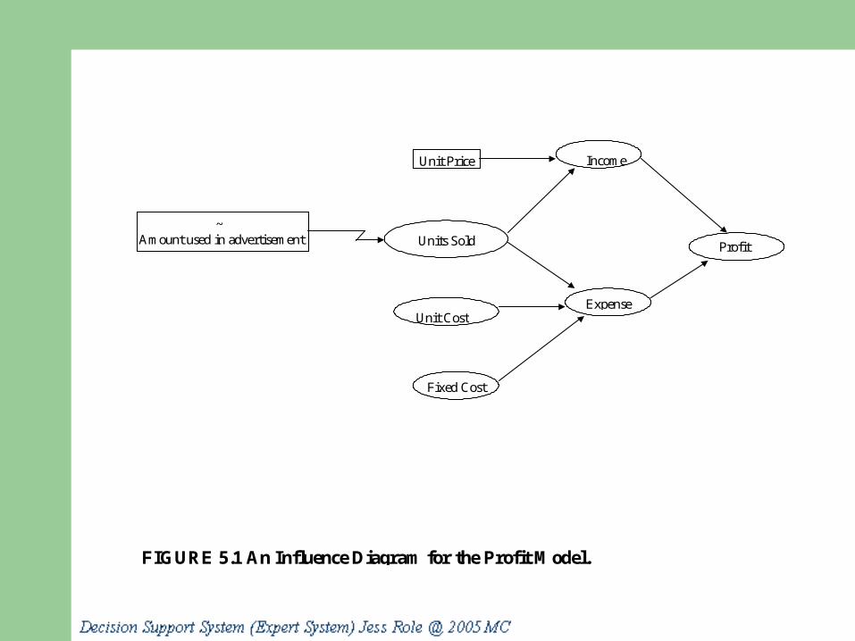
FIGURE 5.1 An Influence Diagram for the Profit Model.
~Amount used in advertisement
Profit
Income
Expense
Unit Price
Units Sold
Unit Cost
Fixed Cost

Analytica Influence Diagram of a Marketing Problem: The Marketing Model (Figure 5.2a)
(Courtesy of Lumina Decision Systems, Los Altos, CA)

Analytica: Price Submodel (Figure 5.2b)(Courtesy of Lumina Decision Systems, Los Altos, CA)

Analytica: Sales Submodel (Figure 5.2c)(Courtesy of Lumina Decision Systems, Los Altos, CA)

MSS Modeling in Spreadsheets
Spreadsheet: most popular end-user modeling tool Powerful functions Add-in functions and solvers Important for analysis, planning, modeling Programmability (macros)
(More)
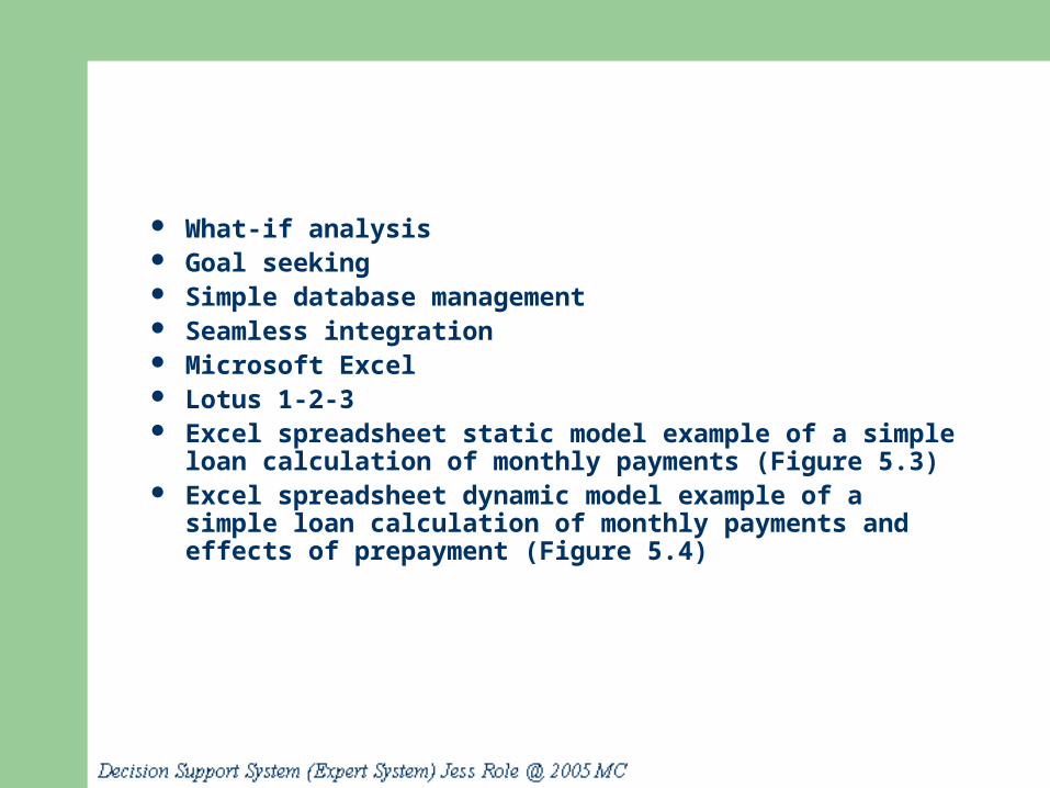
What-if analysis Goal seeking Simple database management Seamless integration Microsoft Excel Lotus 1-2-3 Excel spreadsheet static model example of a simple loan
calculation of monthly payments (Figure 5.3) Excel spreadsheet dynamic model example of a simple loan
calculation of monthly payments and effects of prepayment (Figure 5.4)

Decision Analysis of Few Alternatives
(Decision Tables and Trees)
Single Goal Situations
Decision tables
Decision trees

Decision Tables
Investment example
One goal: maximize the yield after one year
Yield depends on the status of the economy
(the state of nature)– Solid growth– Stagnation– Inflation

1. If solid growth in the economy, bonds yield 12%; stocks 15%; time deposits 6.5%
2. If stagnation, bonds yield 6%; stocks 3%; time deposits 6.5%
3. If inflation, bonds yield 3%; stocks lose 2%; time deposits yield 6.5%
Possible Situations
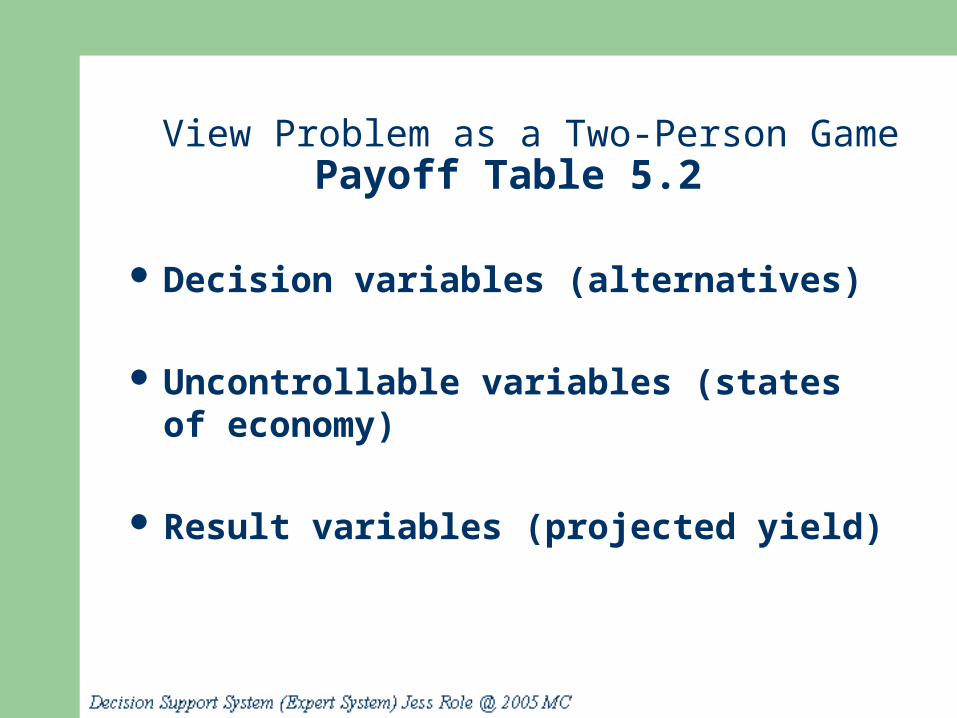
View Problem as a Two-Person GamePayoff Table 5.2
Decision variables (alternatives)
Uncontrollable variables (states of economy)
Result variables (projected yield)

Table 5.2: Investment Problem Decision Table Model
States of Nature
Solid Stagnation Inflation
Alternatives Growth
Bonds 12% 6% 3%
Stocks 15% 3% -2%
CDs 6.5% 6.5% 6.5%

Treating Uncertainty
Optimistic approach
Pessimistic approach

Treating Risk
Use known probabilities (Table 5.3)
Risk analysis: compute expected values
Can be dangerous

Table 5.3: Decision Under Risk and Its Solution
Solid Stagnation Inflation ExpectedGrowth Value
Alternatives .5 .3 .2
Bonds 12% 6% 3% 8.4% *
Stocks 15% 3% -2% 8.0%
CDs 6.5% 6.5% 6.5% 6.5%

Decision Trees
Other methods of treating risk– Simulation– Certainty factors– Fuzzy logic
Multiple goals
Yield, safety, and liquidity (Table 5.4)

Table 5.4: Multiple Goals
Alternatives Yield Safety Liquidity
Bonds 8.4% High High
Stocks 8.0% Low High
CDs 6.5% Very High High
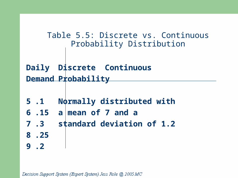
Table 5.5: Discrete vs. Continuous Probability Distribution
Daily Discrete Continuous
Demand Probability
5 .1 Normally distributed with
6 .15 a mean of 7 and a
7 .3 standard deviation of 1.2
8 .25
9 .2

Optimization via Mathematical Programming
Linear programming (LP)
Used extensively in DSS
Mathematical Programming Family of tools to solve managerial problems in allocating
scarce resources among various activities to optimize a measurable goal

LP Allocation Problem Characteristics
1. Limited quantity of economic resources
2. Resources are used in the production of products or services
3. Two or more ways (solutions, programs) to use the resources
4. Each activity (product or service) yields a return in terms of the goal
5. Allocation is usually restricted by constraints

LP Allocation Model
Rational economic assumptions1. Returns from allocations can be compared in a common unit
2. Independent returns
3. Total return is the sum of different activities’ returns
4. All data are known with certainty
5. The resources are to be used in the most economical manner
Optimal solution: the best, found algorithmically

Linear Programming
Decision variables Objective function Objective function coefficients Constraints Capacities Input-output (technology) coefficients
Line

Lindo LP Product-Mix ModelDSS in Focus 5.4
<< The Lindo Model: >>
MAX 8000 X1 + 12000 X2
SUBJECT TO
LABOR) 300 X1 + 500 X2 <= 200000
BUDGET) 10000 X1 + 15000 X2 <= 8000000
MARKET1) X1 >= 100
MARKET2) X2 >= 200
END

<< Generated Solution Report >>
LP OPTIMUM FOUND AT STEP 3
OBJECTIVE FUNCTION VALUE
1) 5066667.00
VARIABLE VALUE REDUCED COST
X1 333.333300 .000000
X2 200.000000 .000000

ROW SLACK OR SURPLUS DUAL PRICES
LABOR) .000000 26.666670
BUDGET) 1666667.000000 .000000
MARKET1) 233.333300 .000000
MARKET2) .000000 -1333.333000
NO. ITERATIONS= 3

RANGES IN WHICH THE BASIS IS UNCHANGED: OBJ COEFFICIENT RANGESVARIABLE CURRENT ALLOWABLE ALLOWABLE COEF INCREASE DECREASE X1 8000.000 INFINITY 799.9998 X2 12000.000 1333.333 INFINITY
RIGHTHAND SIDE RANGES ROW CURRENT ALLOWABLE ALLOWABLE RHS INCREASE DECREASE LABOR 200000.000 50000.000 70000.000 BUDGET 8000000.000 INFINITY 1666667.000MARKET1 100.000 233.333 INFINITYMARKET2 200.000 140.000 200.000

Heuristic Programming Cuts the search Gets satisfactory solutions more quickly and less expensively Finds rules to solve complex problems Finds good enough feasible solutions to complex problems Heuristics can be
– Quantitative– Qualitative (in ES)

When to Use Heuristics
1. Inexact or limited input data
2. Complex reality
3. Reliable, exact algorithm not available
4. Computation time excessive
5. To improve the efficiency of optimization
6. To solve complex problems
7. For symbolic processing
8. For making quick decisions

Advantages of Heuristics
1. Simple to understand: easier to implement and explain
2. Help train people to be creative
3. Save formulation time
4. Save programming and storage on computers
5. Save computational time
6. Frequently produce multiple acceptable solutions
7. Possible to develop a solution quality measure
8. Can incorporate intelligent search
9. Can solve very complex models

Limitations of Heuristics
1. Cannot guarantee an optimal solution
2. There may be too many exceptions
3. Sequential decisions might not anticipate future consequences
4. Interdependencies of subsystems can influence the whole system
Heuristics successfully applied to vehicle routing

Simulation
Technique for conducting experiments with a computer on a model of a management system
Frequently used DSS tool

Major Characteristics of Simulation
Imitates reality and capture its richness
Technique for conducting experiments
Descriptive, not normative tool
Often to solve very complex, risky problems

Advantages of Simulation
1. Theory is straightforward
2. Time compression
3. Descriptive, not normative
4. MSS builder interfaces with manager to gain intimate knowledge of the problem
5. Model is built from the manager's perspective
6. Manager needs no generalized understanding. Each component represents a real problem component
(More)

7. Wide variation in problem types
8. Can experiment with different variables
9. Allows for real-life problem complexities
10. Easy to obtain many performance measures directly
11. Frequently the only DSS modeling tool for nonstructured problems
12. Monte Carlo add-in spreadsheet packages (@Risk)

Limitations of Simulation
1. Cannot guarantee an optimal solution
2. Slow and costly construction process
3. Cannot transfer solutions and inferences to solve other problems
4. So easy to sell to managers, may miss analytical solutions
5. Software is not so user friendly

Simulation Methodology
Model real system and conduct repetitive experiments1. Define problem
2. Construct simulation model
3. Test and validate model
4. Design experiments
5. Conduct experiments
6. Evaluate results
7. Implement solution

Simulation Types
Probabilistic Simulation– Discrete distributions– Continuous distributions– Probabilistic simulation via Monte Carlo technique – Time dependent versus time independent simulation– Simulation software– Visual simulation– Object-oriented simulation

Multidimensional Modeling
Performed in online analytical processing (OLAP) From a spreadsheet and analysis perspective 2-D to 3-D to multiple-D Multidimensional modeling tools: 16-D + Multidimensional modeling - OLAP (Figure 5.6) Tool can compare, rotate, and slice and dice
corporate data across different management viewpoints

Entire Data Cube from a Query in PowerPlay (Figure 5.6a)(Courtesy Cognos Inc.)

Graphical Display of the Screen in Figure 5.6a (Figure 5.6b)
(Courtesy Cognos Inc.)

Environmental Line of Products by Drilling Down (Figure 5.6c)
(Courtesy Cognos Inc.)

Drilled Deep into the Data: Current Month, Water Purifiers, Only in North America (Figure 5.6d)
(Courtesy Cognos Inc.)

Visual Spreadsheets
User can visualize models and formulas with influence diagrams
Not cells--symbolic elements

Visual Interactive Modeling (VIS) and Visual Interactive Simulation (VIS)
Visual interactive modeling (VIM) (DSS In Action 5.8)
Also called– Visual interactive problem solving– Visual interactive modeling– Visual interactive simulation
Use computer graphics to present the impact of different management decisions.
Can integrate with GIS Users perform sensitivity analysis Static or a dynamic (animation) systems (Figure 5.7)

Generated Image of Traffic at an Intersection from the Orca Visual Simulation Environment (Figure 5.7)
(Courtesy Orca Computer, Inc.)

Visual Interactive Simulation (VIS)
Decision makers interact with the simulated model and watch the results over time
Visual interactive models and DSS – VIM (Case Application W5.1 on book’s Web site)– Queueing

Quantitative Software Packages-OLAP
Preprogrammed models can expedite DSS programming time Some models are building blocks of other models
– Statistical packages– Management science packages– Revenue (yield) management– Other specific DSS applications
including spreadsheet add-ins
Model Base Management
MBMS: capabilities similar to that of DBMS But, there are no comprehensive model base management
packages Each organization uses models somewhat differently There are many model classes Within each class there are different solution approaches Some MBMS capabilities require expertise and reasoning

Desirable Capabilities of MBMS
Control Flexibility Feedback Interface Redundancy reduction Increased consistency

MBMS Design Must Allow the DSS User to:
1. Access and retrieve existing models.
2. Exercise and manipulate existing models
3. Store existing models
4. Maintain existing models
5. Construct new models with reasonable effort

Modeling languages Relational MBMS Object-oriented model base and its management Models for database and MIS design and their
management
SUMMARY
Models play a major role in DSS Models can be static or dynamic Analysis is under assumed certainty, risk, or
uncertainty– Influence diagrams– Spreadsheets– Decision tables and decision trees
Spreadsheet models and results in influence diagrams Optimization: mathematical programming
(More)

Linear programming: economic-based Heuristic programming Simulation - more complex situations Expert Choice Multidimensional models - OLAP
(More)

Quantitative software packages-OLAP (statistical, etc.) Visual interactive modeling (VIM) Visual interactive simulation (VIS) MBMS are like DBMS AI techniques in MBMS