1

Chapter 5. Magnetostatics and Electromagnetic

Induction

5.1 Magnetic Field of Steady Currents

The Lorentz force law

The magnetic force in a charge q, moving with velocity v in a magnetic field B in a magnetic field

is

In the presence of both electric and magnetic fields, the net force on q would be

[ ]

This rather fundamental equation known as Lorentz force law tells us precisely how electric and

magnetic fields act on a moving charged particle.

Cyclotron motion

The archetypical motion of a charged particle in a magnetic field is circular, with the magnetic

force providing the centripetal acceleration. In Fig. 5.1 a uniform magnetic field is aligned in the

z direction, and a particle of charge q and mass m is moving with a velocity at .

Using Eq. 5.2 we come up with the equation of motion of this particle,

{

Differentiating the first equation with time and then using the second equation, we get

(

)

(5.4)

zBeB

F

v

Rx

y

(5.1)

(5.2)

Fig 5.1

(5.3)

2

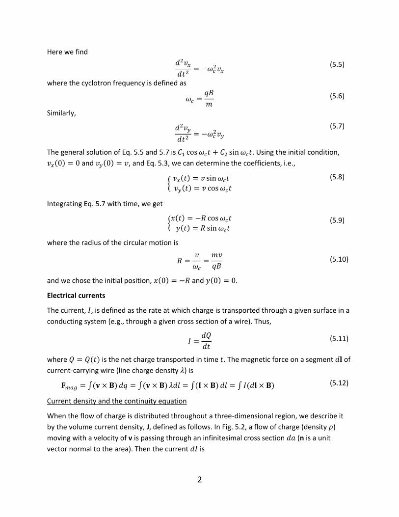
Here we find

where the cyclotron frequency is defined as

Similarly,

The general solution of Eq. 5.5 and 5.7 is . Using the initial condition,

and , and Eq. 5.3, we can determine the coefficients, i.e.,

{

Integrating Eq. 5.7 with time, we get

{

where the radius of the circular motion is

and we chose the initial position, and .

Electrical currents

The current, , is defined as the rate at which charge is transported through a given surface in a

conducting system (e.g., through a given cross section of a wire). Thus,

where is the net charge transported in time . The magnetic force on a segment of

current-carrying wire (line charge density ) is

∫ ∫ ∫ ∫

Current density and the continuity equation

When the flow of charge is distributed throughout a three-dimensional region, we describe it

by the volume current density, J, defined as follows. In Fig. 5.2, a flow of charge (density )

moving with a velocity of v is passing through an infinitesimal cross section (n is a unit

vector normal to the area). Then the current is

(5.5)

(5.6)

(5.8)

(5.9)

(5.7)

(5.10)

(5.11)

(5.12)

3

(5.13)

Here the volume current density

Is the current per unit area perpendicular to flow.

The current through an arbitrarily shaped surface area S may be written as

∫

Applying the equation to an arbitrary closed surface S, we can obtain the electric current

entering V (the volume enclosed by S),

∮ ∫

The first integral has a minus sign because the surface normal n is outward while the current is

inward, and the last integral is obtained through the use of the divergence theorem. Here is

equal to the rate at which charge is transported into V:

∫

∫

Equations 5.16 and 5.17 may be equated:

∫ (

)

Since V is completely arbitrary, we get the continuity equation

This relation has its origin in the fact that charge can neither be created nor destroyed, i.e., this

is the precise mathematical statement of local charge conservation.

dtv

da

dtvn

n

dadI nJ

Fig 5.2

(5.14)

(5.15)

(5.16)

(5.17)

(5.18)

(5.19)

4

Steady current

Steady-state magnetic phenomena are characterized by no change in the net charge density in

space. Consequently in magnetostatics Eq. 5.19 reduces to

A steady current refers to a continuous flow that has been going on forever, without change

and without charge filing up anywhere. Steady currents produce magnetic fields that are

constant in time.

Ohm’s law and conductivity

It is found experimentally that in a metal at constant temperature the current density J is

linearly proportional to the electric field (Ohm’s law):

The constant of proportionality is called the conductivity.

Biot and Savart law: The magnetic induction of a steady current

The magnetic induction of a steady line current is given by the Biot-Savart law:

∫

| |

The constant is called the permeability of free space:

N/A2

B due to a current through a long straight wire

We find the magnetic induction at a distance R from a long straight wire carrying a steady

current I (Fig. 5.4). In the diagram points out of the page, and has the magnitude

| |

ld Bd

x

I

ld

R x

Il

(5.21)

(5.20)

(5.22)

Fig 5.3 Elemental magnetic induction dB

due to current element Idl

(5.23)

Fig 5.4

(5.24)

5

Therefore, the magnitude of B is given by

| |

∫

Since , the integral can be written as

∫

∫

Thus the lines of magnetic induction are concentric circles around the wire.

Forces on current-carrying conductors

The elemental force experienced by a current element in the presence of a magnetic

induction B (Eq. 5.12) is

If the external field B is due to a closed current loop #2 with current , then the total force

which a closed current loop #1 with current experiences is

∮∮

| |

where is the vector distance from line element to . Manipulating the integrand,

| | (

| | )

| |

The integral of the first term over the loop #1 vanishes because

∮

| | ∮

| | ∮ (

| |)

Now we have a symmetric expression for Eq. 5.28

∮∮

| |

This explicitly satisfies the Newton’s third law.

As an application, we find the force between two long, parallel wires a distance d apart,

carrying currents and . The field at (2) due to (1) is

(5.25)

(5.26)

(5.27)

(5.28)

(5.29)

(5.30)

(5.31)

(5.32)

6

which is normal to the direction of . Thus, the magnitude of the force is

∫

The total force is infinite, but the force per unit length is

The force is attractive (repulsive) if the currents flow in the same (opposite) directions.

The divergence and Curl of B

The Biot-Savart law for the general case of a volume current reads

∫

| |

This is the magnetic analog of the Coulomb electric field. With the identity,

, we manipulate the integrand,

| |

| | [

( )

| |]

( )

| | [

( )

| |] (5.36)

Then we find

∫

| |

From this equation it follows immediately that the divergence of B vanishes:

We now calculate the curl of B:

∫

| |

With the identity ,

∫ (

| |)

∫ (

| |)

(5.40)

Using

(

| |) (

| |)

(5.33)

(5.34)

(5.35)

(5.37)

(5.38)

(5.39)

(5.41)

7

and

(

| |)

we rewrite Eq. 5.40 as

∫ (

| |)

Integration by parts yields

∫

| |

For magnetostatics , therefore we obtain

Ampere’s law

Using Stokes’s theorem we can transform Eq. 5.45 into an integral form:

∫

∫

Is transforming into

∮ ∫

which simply says that the line integral of B around a closed path is equal to times the total

current through the closed path, i.e.,

∮

Ampere’s law is useful for calculation of the magnetic induction in highly symmetric simulation.

For example, the magnetic field of an infinite straight wire carrying current has a nonzero curl

(Fig. 5.5). We know the direction of B is circumferential. By symmetry the magnitude of B is

constant around a circular path of radius r. Ampere’s law gives

∮

Thus

I

C

r

B

z

(5.42)

(5.43)

(5.44)

(5.45)

(5.46)

(5.47)

(5.48)

Fig 5.5

(5.49)

8

Vector potential

Since the divergence of any curl is zero (i.e., for an arbitrary vector field ), it is

reasonable to assume that the magnetic induction may be written

The only other requirement placed on is that

Using the identity and specifying that yields

Integrating each rectangular component and using the solution for Poisson’s equation as a

guide leads to

∫

| |

We have, in fact, already found this integral form in Eq. 5.37.

Vector potential and magnetic induction for a circular current loop

We consider the problem of a circular loop of radius a, lying in the x-y plane, centered at the

origin, and carrying a current I, as shown in Fig. 5.6. Due to the cylindrical geometry, we may

choose the observation point P in the x-z plane ( ) without loss of generality. The

expression for the vector potential Eq. 5.53 may be applied to the current circuit by making the

substitution: . Thus

∫

| |

where . Then, Eq. 5.54 becomes

∫

z

x

y

)0,,( rP

a

'Idx

'

r

(5.50)

(5.51)

(5.52)

(5.53)

Fig 5.6

(5.54)

(5.55)

9

Since the azimuthal integration in Eq. 5.54 is symmetric about , the component

vanishes. This leaves only the component, which is . Therefore

∫

For or ,

√ (

)

Hence

√ ∫ (

)

The integration results in

The components of magnetic induction,

{

( )

( )

The fields far from the loop (for )

{

where is the magnetic dipole moment of the loop. Comparison with the

electrostatic dipole fields shows that the magnetic fields are dipole in character.

The fields on the z axis (for )

For , hence

For , , therefore Eq. 5.60 is valid on any points on

the z axis.

(5.56)

(5.57)

(5.58)

(5.59)

(5.60)

10

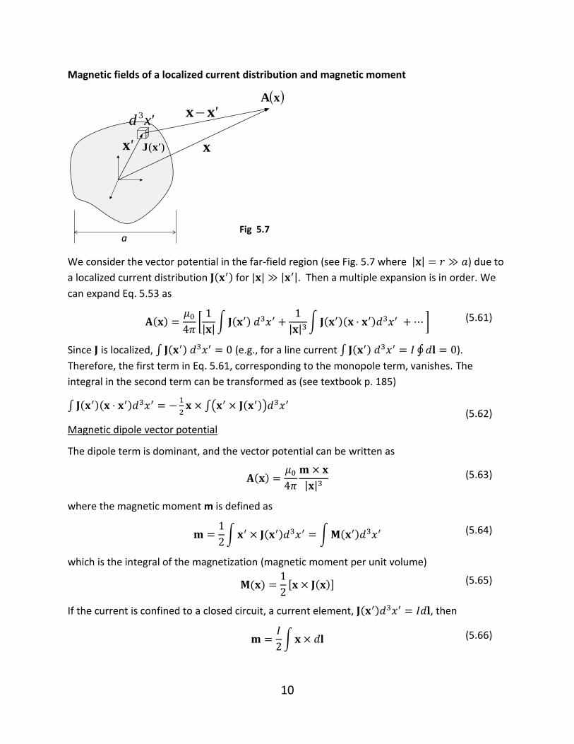
Magnetic fields of a localized current distribution and magnetic moment

We consider the vector potential in the far-field region (see Fig. 5.7 where | | ) due to

a localized current distribution for | | | |. Then a multiple expansion is in order. We

can expand Eq. 5.53 as

[

| |∫

| | ∫ ]

Since is localized, ∫ (e.g., for a line current ∫ ∮ ).

Therefore, the first term in Eq. 5.61, corresponding to the monopole term, vanishes. The

integral in the second term can be transformed as (see textbook p. 185)

∫

∫( )

Magnetic dipole vector potential

The dipole term is dominant, and the vector potential can be written as

| |

where the magnetic moment m is defined as

∫ ∫

which is the integral of the magnetization (magnetic moment per unit volume)

[ ]

If the current is confined to a closed circuit, a current element, , then

∫

'xx

'x x

xA

x'd 3

)( 'xJ

aFig 5.7

(5.61)

(5.62)

(5.63)

(5.64)

(5.65)

(5.66)

11

For a plane loop, is perpendicular to the plane of the loop. Since

| | is the area of the

triangle defined by the two ends of and the origin, the loop integral gives the total area of

the loop. Hence the magnetic moment has magnitude,

regardless of the shape of the circuit.

Dipole magnetic induction

The magnetic induction can be determined by taking the curl of Eq. 5.63.

(

| | )

[ (

| | )

| | (

| | )

| | ] (5.68)

Since

| | for | | and m is independent of x, the first three terms vanish. The last

term can be transformed by noting that

(

| | )

| |

| |

hence

| |

| |

| |

Finally,

[

| | ]

Here is a unit vector in the direction .

Force and torque on a localized current distribution in an external B

The magnetic force is given by (eq. 5.12)

∫ ∫

Similarly the total torque on the current distribution is

∫ ∫

If the current distribution is localized and the magnetic induction varies slowly over the region

of current, we can expand B in a Taylor series. A component of B takes the form,

(5.69)

(5.70)

(5.71)

(5.67)

(5.72)

(5.73)

(5.74)

12

Magnetic force

The -th component of the force Eq. 5.72 becomes

∑ [ ∫ ∫

]

We already know ∫ for a localized current, so the first term vanishes. Now the

second term is dominant and becomes

∑ [∫ (

)

] ∑

This can be written in a vector from as

Since , the lowest order force on a localized current distribution in an external

magnetic field B is

Magnetic torque

Keeping on the leading term in Eq. 5.74, Eq 5.73 can be written as

∫[ ]

The first integral has the same form of the second term of Eq. 5.75. The second integral

vanishes because ∫ if . Therefore, the leading term in the torque is

5.2 Magnetic Fields in Matter

Three mechanisms of macroscopic magnetic-moment distribution

Matter on the atomic level is made up of relatively stationary nuclei surrounded by electrons in

various orbits. There are three mechanisms whereby matter may acquire a macroscopic

magnetic-moment distribution. By macroscopic we mean averaged over a large number of

atoms. This distribution is characterized by the magnetic moment per unit volume , called the

magnetization (see Eq. 5.65):

∑ ⟨ ⟩

where is the average number per unit volume of atoms or molecules of type and ⟨ ⟩ is

the average atomic or molecular moment in a small volume at the point x. The three

mechanisms are as follows:

(5.75)

(5.76)

(5.77)

(5.78)

(5.79)

(5.80)

(5.81)

13

Diamagnetism – The application of a magnetic induction to a diamagnetic medium

induces currents within the atomic systems, and these in turn lead to a macroscopic

magnetic-moment density opposite in direction to the applied field.

Paramagnetism – The electrons’ total (orbital + spin) angular momenta may be arranged

so as to give rise to a net magnetic moment within each atomic system.

Ferromagnetism – Ferromagnetic materials (e.g., iron, cobalt, nickel) have remarkable

atomic properties. First, several electrons in an isolated atom have their intrinsic angular

momenta lined up. Second, within solid ferromagnets, there are very strong quantum-

mechanical forces tending to make the intrinsic angular momenta of neighboring atoms

line up. These results in domains of macroscopic size having net magnetizations.

Vector potential due to magnetization

The vector potential due to a magnetic moment (Eq. 5.63) is

| |

| |

Hence we write

∫

| |

∫ [

( )

| |]

∫

( )

| |

The first volume integral can be transformed to a surface integral:

∫ [

| |]

∫

| |

Observing that at infinity, we note that this integral vanishes. Thus we have

∫

| |

Macroscopic equations

Comparing Eq. 5.85 with our usual equation for A (Eq. 5.53) in terms of current density, J can be

replaced entirely by an effective current density

In general, all current distributions can be considered as consisting of two parts:

(magnetization current) and (free current). Hence we write our basic equation for B as follows:

(5.82)

(5.83)

(5.84)

(5.85)

(5.86)

(5.87)

14

Rewriting this equation, we obtain

(

)

Here we defined a new macroscopic field H, called magnetic field,

Then the macroscopic equations are

Magnetic susceptibility and permeability

To complete the description of macroscopic magnetostatics, it is essential to have a relationship

between B and H or, equivalently, a relationship between M and H (or B). In a large class of

materials there exists an approximately linear relationship between M and H. If the material is

isotropic as well as linear,

where is called the magnetic susceptibility (paramagnetic for and diamagnetic for

). It is generally safe to say that for paramagnetic and diamagnetic materials is quite

small: | | . A linear relationship between M and H implies also a linear relationship

between B and H:

where the permeability is obtained from Eqs. 5.89, 5.90, and 5.91 and

The ferromagnetic substances are characterized by a possible permanent magnetization. These

materials are not linear, so that Eqs. 5.90 and 5.91 with constant and do not apply.

Instead, a nonlinear functional relationship is applied:

(5.88)

(5.89)

(5.90)

(5.90)

(5.91)

(5.92)

(5.93)

Fig 5.8 Hysteresis loop

15

The curve of Fig. 5.8 is called the hysteresis loop of the material. is known as the retentivity

or remnance; the magnitude is called the coercive force or coercivity of the material. Once

is sufficient to produce saturation, the hysteresis loop does not change shape with

increasing .

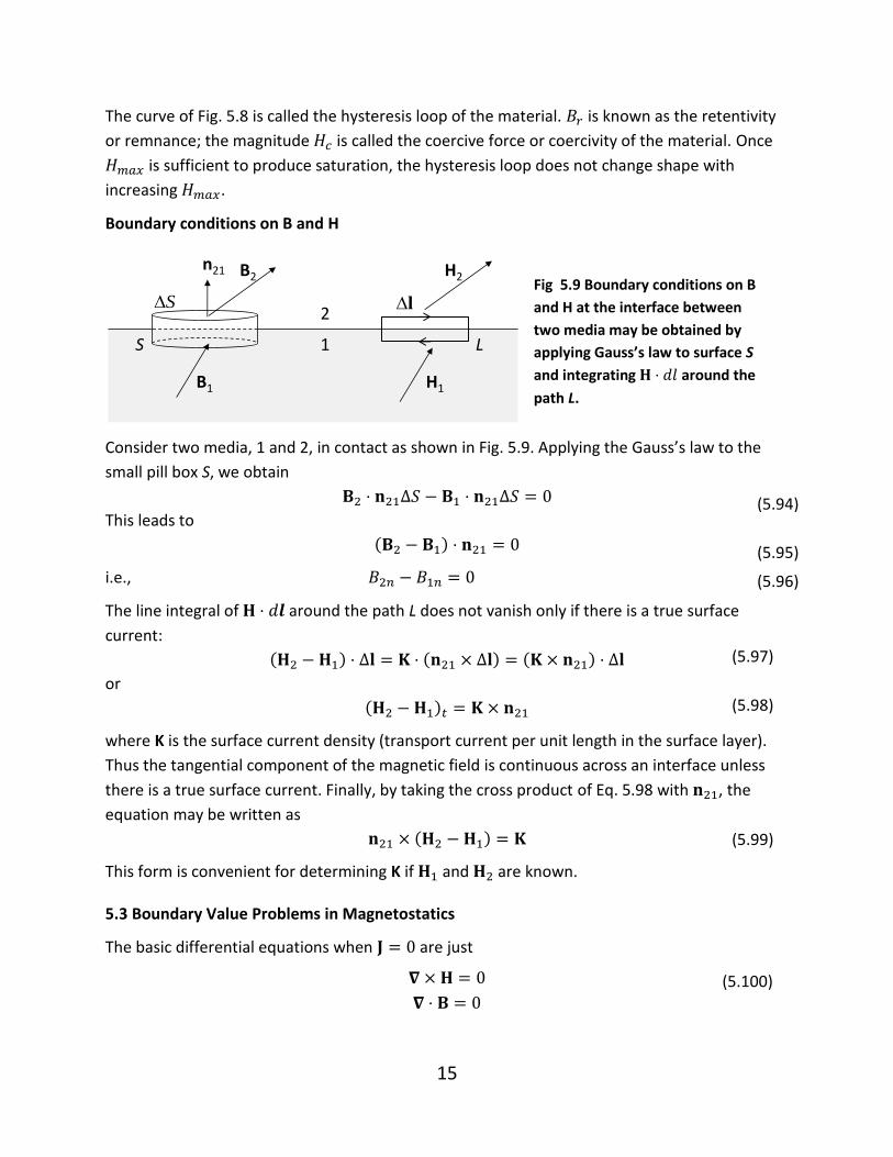
Boundary conditions on B and H

Consider two media, 1 and 2, in contact as shown in Fig. 5.9. Applying the Gauss’s law to the

small pill box S, we obtain

This leads to

i.e.,

The line integral of around the path L does not vanish only if there is a true surface

current:

or

where K is the surface current density (transport current per unit length in the surface layer).

Thus the tangential component of the magnetic field is continuous across an interface unless

there is a true surface current. Finally, by taking the cross product of Eq. 5.98 with , the

equation may be written as

This form is convenient for determining K if and are known.

5.3 Boundary Value Problems in Magnetostatics

The basic differential equations when are just

n21

1

2

B2

H1B1

H2

LS

S lFig 5.9 Boundary conditions on B

and H at the interface between

two media may be obtained by

applying Gauss’s law to surface S

and integrating around the

path L.

(5.95)

(5.94)

(5.96)

(5.97)

(5.99)

(5.98)

(5.100)

16

The first equation permits us immediately to defined a magnetic scalar potential such that

Just as in electrostatics. The second equation can be written as

Hence we conclude that satisfies the Poisson equation

with the effective magnetic-charge density,

If there is no boundary surfaces, the solution for is

∫

| |

In the event that we have a surface of discontinuity, we need to calculate an effective magnetic

surface-charge density . Making use of Gauss’s theorem to a small pill box at the interface,

we find

where is a unit vector pointing from region 1 to region 2. If and , Eq. 5.106

reduces to

Uniformly magnetized sphere

We consider a sphere of radius with a uniform permanent magnetization in vacuum

(Fig. 5.10). The simplest way of solving this problem is in terms of the scalar magnetic potential.

Since , satisfies Laplace's equation,

The magnetic surface-charge density is

zM eM 0

za

r

(5.101)

(5.102)

(5.103)

(5.104)

(5.105)

(5.106)

(5.107)

(5.108)

(5.109)

Fig 5.10

17

Inside and outside potential

From the azimuthal symmetry of the geometry we can take the solution to be of the form:

(i) Outside:

∑[

]

∑

At large distances from the sphere, i.e., for the region , the potential is given by

Accordingly, we can immediately set all equal to zero.

(ii) Inside:

∑

Since is finite at , terms must vanish.

Boundary conditions at

(i) Tangential H:

|

|

(5.113)

or (5.114)

(ii) Normal B:

|

|

(5.115)

Applying boundary condition (i) (Eq. 5.114) tells us that

∑

∑

We deduce from this that

We apply boundary condition (ii) results in

∑[

]

We deduce from this that

{

(5.112)

(5.111)

Fig 3.2.

(5.110)

(5.116)

(5.118)

(5.119)

(5.120)

(5.117)

18

The equations 4.57 and 4.60 can be satisfied only if

{

From Eqs. 5.117 and 5.120, we can deduce that for all . The potential is

therefore

{

An alternative way to calculate is

∫

| |

Using the addition theorem (Eq. 3.68) and the azimuthal symmetry

| | ∑

∑

we obtain

∑

∫

where are smaller and larger of . Letting , we find

∑

∫

Applying the orthogonality condition for the Legendre polynomials, we obtain

This is equal to Eq. 5.123.

Outside B and H

Outside the sphere is the potential of a dipole with dipole moment,

(5.121)

(5.122)

(5.123)

(5.128)

(5.124)

(3.68)

(5.125)

(5.126)

(5.127)

19

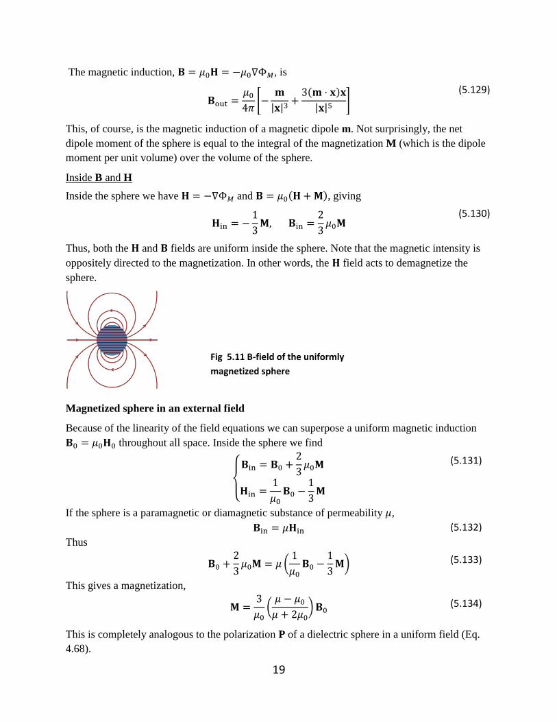
The magnetic induction, , is

[

| |

| | ]

This, of course, is the magnetic induction of a magnetic dipole m. Not surprisingly, the net

dipole moment of the sphere is equal to the integral of the magnetization M (which is the dipole

moment per unit volume) over the volume of the sphere.

Inside B and H

Inside the sphere we have and , giving

Thus, both the and fields are uniform inside the sphere. Note that the magnetic intensity is

oppositely directed to the magnetization. In other words, the field acts to demagnetize the

sphere.

Magnetized sphere in an external field

Because of the linearity of the field equations we can superpose a uniform magnetic induction

throughout all space. Inside the sphere we find

{

If the sphere is a paramagnetic or diamagnetic substance of permeability ,

Thus

(

)

This gives a magnetization,

(

)

This is completely analogous to the polarization P of a dielectric sphere in a uniform field (Eq.

4.68).

(5.129)

(5.130)

Fig 5.11 B-field of the uniformly

magnetized sphere

(5.131)

(5.132)

(5.133)

(5.134)

20

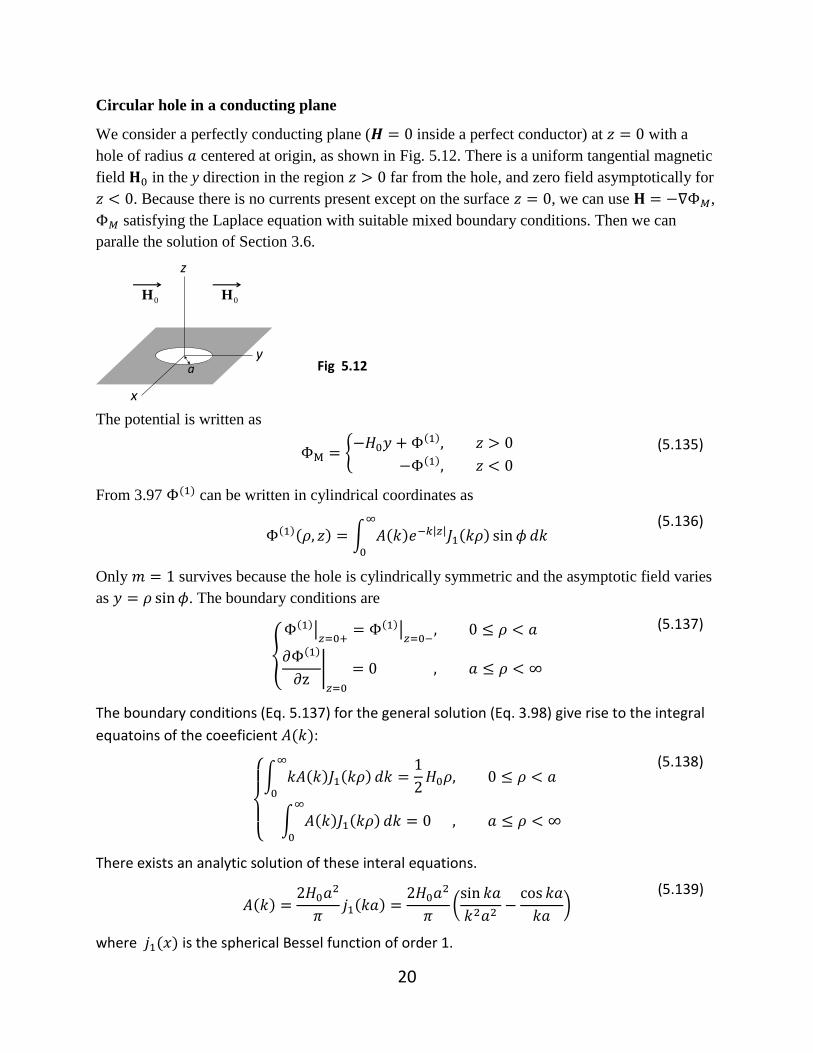
Circular hole in a conducting plane

We consider a perfectly conducting plane ( inside a perfect conductor) at with a

hole of radius centered at origin, as shown in Fig. 5.12. There is a uniform tangential magnetic

field in the y direction in the region far from the hole, and zero field asymptotically for

. Because there is no currents present except on the surface , we can use ,

satisfying the Laplace equation with suitable mixed boundary conditions. Then we can

paralle the solution of Section 3.6.

The potential is written as

{

From 3.97 can be written in cylindrical coordinates as

∫ | |

Only survives because the hole is cylindrically symmetric and the asymptotic field varies

as . The boundary conditions are

{

|

|

|

The boundary conditions (Eq. 5.137) for the general solution (Eq. 3.98) give rise to the integral

equatoins of the coeeficient :

{

∫

∫

There exists an analytic solution of these interal equations.

(

)

where is the spherical Bessel function of order 1.

z

x

ya

0H 0H

Fig 5.12

(5.135)

(5.136)

(5.137)

(5.139)

(5.138)

21

In the far-feld region, i.e., in the region for | | and/or , the integral in Eq. 5.136 is mainly

determined by the contributions around , more precisely, for

. The expansion of

for small takes the form

[

]

The leading term gives rise to the asymptotic potential

falling off with distance as and having an effective electric dipole moment,

where for and for . In the opening, the tangential and normal components of

the magnetic fieds are

√

5.4 Electromagnetic Induction

Faraday’s law

Fig 5.13

Figure 5.13 illustrates the observation made by Faraday. He showed that changing the magnetic

flux through a circuit induce a current in it. This could be accomplished by (a) moving the circuit

in and out of the magnet, (b) moving the magnet toward or away from the circuit, or (c)

changing the strength of the magnetic field. These observations can be expressed by the flux

rule:

B

Iv

B

Iv

B

I

changingmagnetic field

(a) (b) (c)

(5.140)

(5.141)

(5.142)

(5.143)

22

where the electromotive force (emf) is defined by the integral of a force per unit charge

∮

( is the electric field in the stationary frame of the circuit) and the magnetic flux is defined

by

∫

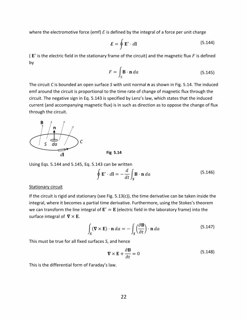
The circuit C is bounded an open surface S with unit normal n as shown in Fig. 5.14. The induced

emf around the circuit is proportional to the time rate of change of magnetic flux through the

circuit. The negative sign in Eq. 5.143 is specified by Lenz’s law, which states that the induced

current (and accompanying magnetic flux) is in such as direction as to oppose the change of flux

through the circuit.

Using Eqs. 5.144 and 5.145, Eq. 5.143 can be written

∮

∫

Stationary circuit

If the circuit is rigid and stationary (see Fig. 5.13(c)), the time derivative can be taken inside the

integral, where it becomes a partial time derivative. Furthermore, using the Stokes’s theorem

we can transform the line integral of (electric field in the laboratory frame) into the

surface integral of .

∫

∫ (

)

This must be true for all fixed surfaces S, and hence

This is the differential form of Faraday’s law.

C

ld

B

S

n

da

(5.144)

Fig 5.14

(5.145)

(5.146)

(5.147)

(5.148)

23

Moving circuit

We consider a circuit moving with a constant velocity v. The force per unit charge on a charge

which is fixed with respect to a given point on the circuit is

assuming Galilean transformation ( , ), then the electric field in a

coordinate frame moving with a velocity v relative to the laboratory frame is

The emf which results from a motion of the circuit is

∮ ∮ ∮(

)

If B is static and the circuit is rigid (i.e., is independent of time), the time derivative can be

taken out of the integral. Then,

∮

∫

(

)

Self-inductance

For a rigid stationary circuit the only changes in flux result from changes in the current:

If is directly proportional to , then the inductance defined as

is constant. Then, the expression for emf becomes

which is an equation of considerable practical importance.

Mutual inductance

Assuming there are n circuits, we can write the flux linking one of these circuits as a sum of

fluxes due to each of the n circuits:

∑

(5.149)

(5.150)

(5.151)

(5.152)

(5.154)

(5.153)

(5.155)

(5.156)

24

The emf induced in the ith circuit can then be written as

∑

If each of the circuits is rigid and stationary,

where we define the mutual inductance

The Neumann formula

The flux

∫ ∫(

∮

( )

| | )

Since

∮ ( )

| | ∮

| |

we can write

∫ (∮

| |)

∮∮

| |

using Stoke’s theorem. Therefore, the mutual inductance is expressed as

∮∮

| |

which is known as Neumann’s formula for the mutual inductance. It is apparent that .

Neumann’s formula is equally applicable to self-inductance:

∮∮

| |

Energy in the magnetic field

Suppose we have a single circuit with a constant current flowing in it. To keep the current

constant, the sources of current must do work. First, we consider the work done on an electron.

When an electron moves with velocity v acted by due to a changing magnetic flux, the

change in energy per unit time is

(5.165)

(5.159)

(5.157)

(5.158)

(5.160)

(5.161)

(5.162)

(5.163)

(5.164)

25

Summing over all the electrons in circuit, we find that the power to maintain the current is

∑

∫

The negative sign follows from the Lenz’s law. Assuming that the electrons form a continuous

charge distribution, the summation can be transformed into a volume integral

∫ ∫(∫ )

where the line element and the unit vector are in the direction of . Therefore, if the flux

change through a circuit carrying a current is , the work done by the source is

∫

∮

If there are multiple circuits carrying the currents, ,

∑

∑ ∮

Energy density in the magnetic field

Suppose that each “circuit” is a closed path in the medium that follows a line of current density.

Then, choosing a large number of contiguous circuits ( ) and replacing with , we

obtain

∫

Using Ampere’s law, we find

∫

Using the vector identity and applying the divergence

theorem, we obtain

∫ ∫

If the field distribution is localized, the surface integral vanishes. Since ,

∫

Assuming that the medium is para- or diamagnetic, i.e., with a constant ,

(5.166)

(5.167)

(5.168)

(5.170)

(5.171)

(5.172)

(5.173)

(5.174)

(5.169)

26

Then, the total magnetic energy becomes

∫

By reasoning similar to that of the electrostatic energy density, we are led to the concept of

energy density in a magnetic field:

Assuming a linear relation between J and A, Eq. 5.170 leads to the magnetic energy

∫

Magnetic energy of coupled circuits

If there are n rigid stationary circuits carrying the currents, , the work done against

the induced emf is given by

∑

Assuming that all currents (and all fluxes) are brought to their final values in concert, i.e., at any

instant of time all currents and all fluxes will be at the same fraction of their final values,

and . Integration of Eq. 5.169 is

∫ ∫

∑

∑

∫

∑

Then, the magnetic energy for rigid circuits and linear media is

∑

From Eqs. 5.156 and 5.159, the magnetic energy can be expressed as

∑∑

(5.175)

(5.178)

(5.176)

(5.179)

(5.180)

(5.181)

(5.182)

27

Forces on rigid circuits

Suppose we allow one of the parts of the system to make a rigid displacement under the

influence of the magnetic forces acting upon it, all currents remaining constant. The mechanical

work done by the force F acting on the system is

where is the change in magnetic energy of the system and is the work done by

external energy sources against the induced emf to keep the current constant. According to Eq.

5.179 and 5.181,

∑

and

∑

Thus,

Then,

or

(

)

The force on the circuit is the gradient of the magnetic energy when is maintained constant.

Force between two rigid circuits carrying constant currents

The magnetic energy is given by

and the force on circuit 2 is

Where the mutual inductance must be written so that it display its dependence on .

Neumann’s formula shows this dependence explicitly, so we may write

∮∮

| |

∮∮

| |

an expression that evidently shows the proper symmetry, i.e., . It is equivalent to

∮∮

[ ]

| |

(5.183)

(5.184)

(5.185)

(5.186)

(5.187)

(5.188)

(5.189)

(5.190)

(5.191)

(5.192)

28

Solenoid and iron rod

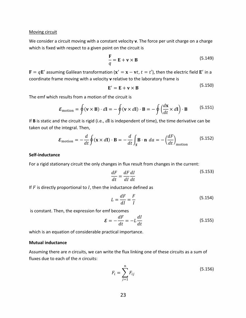
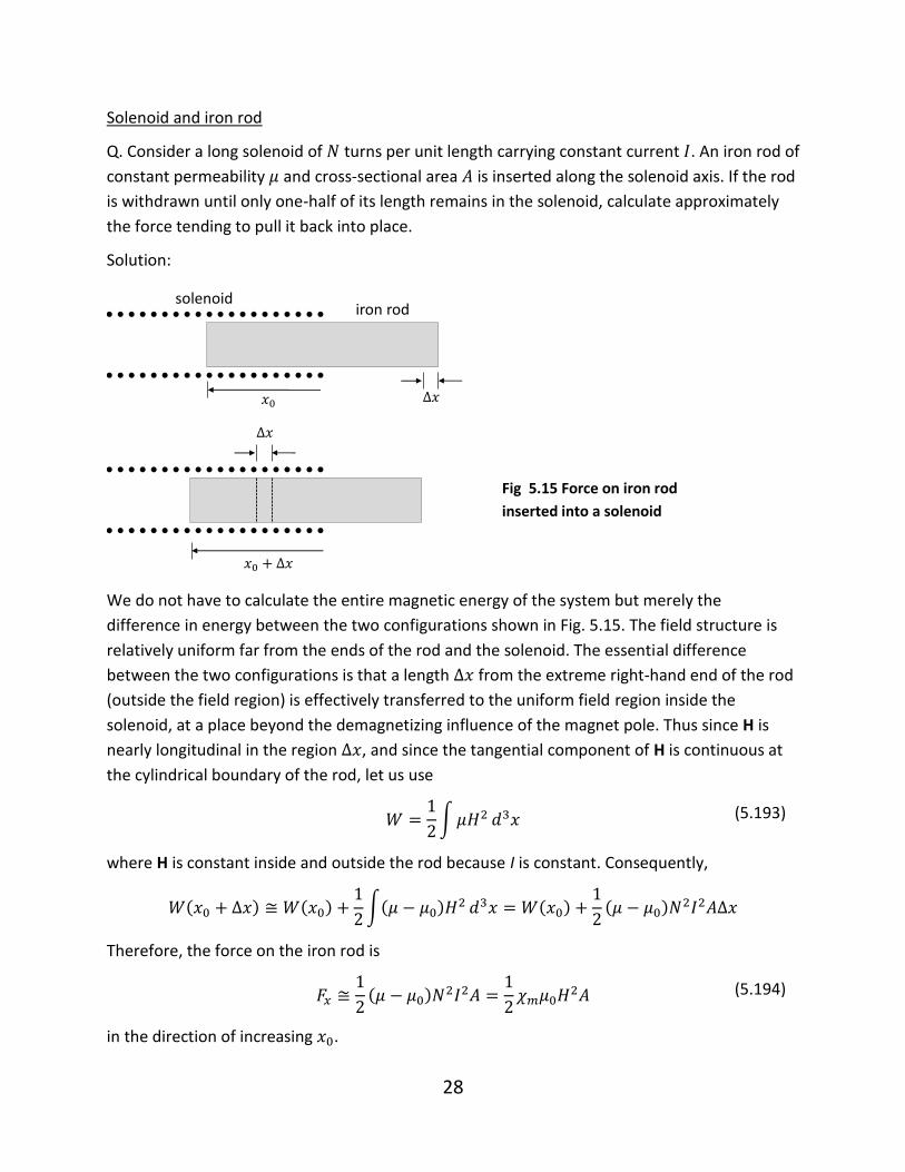
Q. Consider a long solenoid of turns per unit length carrying constant current . An iron rod of

constant permeability and cross-sectional area is inserted along the solenoid axis. If the rod

is withdrawn until only one-half of its length remains in the solenoid, calculate approximately

the force tending to pull it back into place.

Solution:

We do not have to calculate the entire magnetic energy of the system but merely the

difference in energy between the two configurations shown in Fig. 5.15. The field structure is

relatively uniform far from the ends of the rod and the solenoid. The essential difference

between the two configurations is that a length from the extreme right-hand end of the rod

(outside the field region) is effectively transferred to the uniform field region inside the

solenoid, at a place beyond the demagnetizing influence of the magnet pole. Thus since H is

nearly longitudinal in the region , and since the tangential component of H is continuous at

the cylindrical boundary of the rod, let us use

∫

where H is constant inside and outside the rod because I is constant. Consequently,

∫

Therefore, the force on the iron rod is

in the direction of increasing .

solenoidiron rod

Fig 5.15 Force on iron rod

inserted into a solenoid

(5.193)

(5.194)