Chapter 5 Explanatory Item Response Models: A Brief ... · Chapter 5 Explanatory Item Response...

J. Hartig, E. Klieme, & D. Leutner (Eds.),Assessment of Competencies in Educational Contexts, 83–110.© 2008 Hogrefe & Huber Publishers

Chapter 5Explanatory Item Response Models: A Brief Introduction�

Mark Wilson, Paul De Boeck, and Claus H. Carstensen

In this chapter we illustrate the use of item response models to analyze data result-ing from the measurement of competencies. These item response models deal with data from an instrument such as a test, an inventory, an attitude scale, or a question-naire – we will call this “test data”. The main purpose of using item response models is the measurement of propensities: specifically, abilities, skills, achievement levels, traits, attitudes, etc. In standard item response modeling each item is modeled with its own set of parameters and in one way or another, the person parameters are also esti-mated – we will call this the “measurement” approach. In a broader approach, which does not contradict but complements the measurement approach, one might want to model how the properties of the items and the persons making the responses lead to the persons’ responses – we will call this the “explanatory” approach (De Boeck & Wilson, 2004). Understanding how the item responses are generated implies that the responses can be explained in terms of properties of items and of persons.

We also take a broader statistical approach than that of standard item response models. It turns out that most extant item response models are special cases of what are called generalized linear or nonlinear mixed models (GLMMs and NLMMs; McCulloch & Searle, 2001). In this chapter, the perspective that is taken on these models is quite sim-ple in its general expression (although it is not necessarily simple in how it is applied to a specific situation) and it has several advantages. We see it as being straightforward because the similarities and differences between models can be described in terms of the kinds of predictors (item properties, person properties, and interactions of item and person properties) and the kinds of weights they have, just as in the familiar regression model. Perhaps the most important feature of the broader approach is that it facilitates the implementation of the explanatory perspective described above. Additional impor-tant advantages we see are that the approach is general and therefore also flexible, and it connects psychometrics strongly to the field of statistics, so that a broader knowledge base and more literature become available.

One can also see this chapter as dealing primarily with repeated observations which

1 Acknowledgements: This chapter has been adapted from the first two chapters of De Boeck and Wilson (2004). We wish to thank the German PISA Consortium, who generously pro-vided the data set used in the example.

84 M. Wilson, P. De Boeck, & C. H. Carstensen

may result from different types of studies. First, they may come from an experiment with factors that are manipulated within persons. The corresponding design is called a within-subjects design in the psychological literature because the covariates (the design factors) vary within individuals. The factors are covariates that one wants to relate to the observations. For example (an example that we will expand upon in later sections), a student’s mathematics competency could be investigated using different types of mathematics problems from different areas of mathematical application. These differ-ent conditions of mathematics items constitute a manipulated factor and a covariate.

Second, these observations may also come from studies with a longitudinal design: repeated observations of the same categorical dependent variable at regular (or irregu-lar) time intervals. The time of observation as such and covariates of time may also be considered observation properties one wants to relate to the observations. Third, and finally, the repeated observations may be responses to the items from a test instrument (thinking of this class broadly as being composed of instruments such as achievement and aptitude tests, attitude scales, behavioral inventories, etc.). Since a test typically consists of more than one item, test data are repeated observations. Test data are just a special case, but given the measurement perspective (the one we described earlier) they are a prominent one.

We have found it helpful to think of test data as being repeated observations that have to be explained by way of properties that co-vary with the observations. This way of thinking can render tests a way of examining theories and less exclusively a matter of measuring. Note that tests with a test design (Embretson, 1985) may be considered ex-periments with a within-subjects design, because the design implies that item properties are varied within the test, just like design factors are manipulated in an experiment.

For the three kinds of data mentioned above (experimental data, longitudinal data, and test data) the person side may also have a design based on the manipulation of some factors not within individuals but between individuals, or based on groups to which people belong: by gender, ethnicity, school, country, etc. When the participants are all drawn from one population (one group), the design is a single-sample design. When they are drawn from different populations (e.g., males and females), the design is a multi-sample design. Another term for the latter is the split-plot design. Thus, for the approach we are following in this chapter, the design can be seen as a single-sample repeated-observations design, or a multi-sample repeated-observations design. More generally, many types of person properties can be included to investigate their effects, not only group properties, but also continuous person properties. For example, one may have external information that transcends the sample design, such as a person’s age.

An important and distinctive feature of the data we will deal with is their categorical nature. The simplest case of a categorical variable is a binary variable. Many tests have only two response categories; however, other tests have more response categories, but they have been recoded into, say, 1 and 0, because one is interested only in whether or not the responses are correct, or whether the test-takers agree or disagree with the statement made by the item. This is why measurement models for binary data are more popular. However, in other cases, there may be more than two response categories which are not recoded into two values. Similarly, observations in general can be made

Explanatory Item Response Models: A Brief Introduction 85

in two or more categories. Where there are more than two categories, the data are called polytomous or multicategorical.

Observation categories can be ordered or unordered. The categories can be ordered because of the way they are defined, as in a rating scale format, or they can be ordered based on the investigator’s conception. The corresponding data are ordered-category data. Examples of categories that are ordered by definition are degree of frequency (e.g., often, sometimes, never), of agreement (e.g., strongly agree, agree, disagree, strongly disagree) and of intensity (e.g., very much, moderately, slightly). Observational catego-ries may also be unordered because nothing in the category definition is ordinal and/or because one has no idea of how the categories relate to some underlying dimension. The difference between the categories is only nominal and therefore they are called nominal categories and the corresponding data are called nominal-category data. For example, in most multiple-choice tests the correct distractor is known to be better than the others, but it is not usually clear how the incorrect responses are ordered with respect to the underlying ability or achievement level. The models in this chapter focus on binary data and ordered-category data. However, binary data will play a more important role in the chapter, since all models for binary data can be extended to other types of categorical data.

The remaining sections are devoted to: (a) a description of the data that will be used to illustrate the new framework; (b) a discussion of data structure; (c) a brief description of the statistical approach we used; (d) a discussion of how the framework helps one to con-ceptualize existing item response models, incorporating an example that goes beyond the usual range of item response models; and (e) a summary of further expansions.

The German Mathematical Literacy Example

We will make use of a sample data set based on the German mathematical literacy test (German PISA Consortium, 2004) to introduce some principles behind the mod-els we will deal with in this chapter. The sample data can be considered test data or experimental data. The instrument is a test of mathematics competency taken from one booklet of a German mathematics test administered to a random sub-sample of the German PISA sample of 15 year-old students in the 2003 administration. The test was developed under the same general guidelines as the PISA mathematics test, where mathematical literacy is a “described variable” with several successive levels of sophis-tication in performing mathematical tasks. These levels are shown in Table 1. There are 881 students in total.


Table 1. PISA levels of mathematical literacy.

Level Description

VI At Level VI students can conceptualise, generalise, and utilise information based on their investigations and modelling of complex problem situations. They can link different information sources and representations and flexibly translate among them. Students at this level are capable of advanced mathematical thinking and reasoning. These students can apply their insight and understanding along with a mastery of symbolic and formal mathematical operations and relationships to develop new approaches and strategies for attacking novel situations. Students at this level can formulate and precisely communicate their actions and reflections regarding their findings, interpretations, arguments, and the appropriateness of these to the original situations.

V At Level V students can develop and work with models for complex situations, identifying constraints and specifying assumptions. They can select, compare, and evaluate appropriate problem-solving strategies for dealing with complex problems related to these models. Students at this level can work strategically using broad, well-developed thinking and reasoning skills, appropriate linked representations, symbolic and formal characterisations, and insight pertaining to these situations. They can reflect on their actions and formulate and communicate their interpretations and reasoning.

IV At Level IV students can work effectively with explicit models for complex concrete situations that may involve constraints or call for making assumptions. They can select and integrate different representations, including symbolic, linking them directly to aspects of real-world situations. Students at this level can utilize well-developed skills and reason flexibly, with some insight, in these contexts. They can construct and communicate explanations and arguments based on their interpretations, arguments, and actions.

III At Level III students can execute clearly described procedures, including those that require sequential decisions. They can select and apply simple problem-solving strategies. Students at this level can interpret and use representations based on different information sources and reason directly from them. They can develop short communications reporting their interpretations, results and reasoning.

II At Level II students can interpret and recognise situations in contexts that require no more than direct inference. They can extract relevant information from a single source and make use of a single representational mode. Students at this level can employ basic algorithms, formulae, procedures, or conventions. They are capable of direct reasoning and making literal interpretations of the results.

I At Level I students can answer questions involving familiar contexts where all relevant information is present and the questions are clearly defined. They are able to identify information and to carry out routine procedures according to direct instructions in explicit situations. They can perform actions that are obvious and follow immediately from the given stimuli.

The test booklet contained 64 dichotomous items; 18 of these items were selected for this example. An example of an item is shown in Figure 1. Each item was constructed


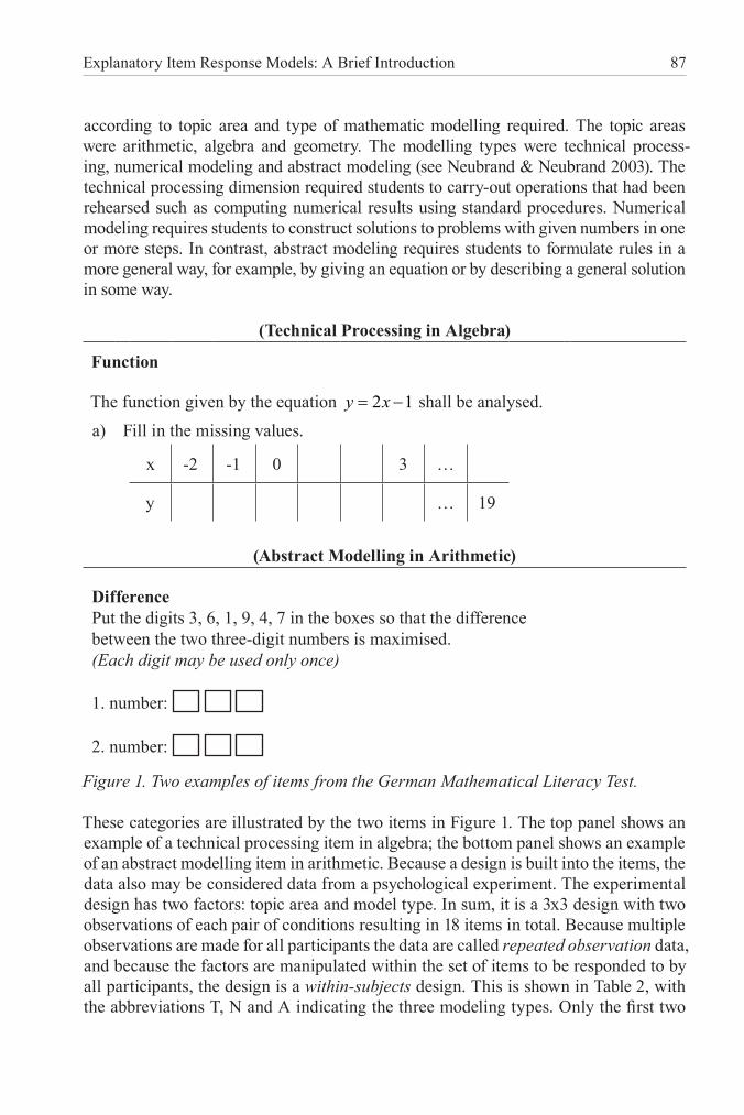
according to topic area and type of mathematic modelling required. The topic areas were arithmetic, algebra and geometry. The modelling types were technical process-ing, numerical modeling and abstract modeling (see Neubrand & Neubrand 2003). The technical processing dimension required students to carry-out operations that had been rehearsed such as computing numerical results using standard procedures. Numerical modeling requires students to construct solutions to problems with given numbers in one or more steps. In contrast, abstract modeling requires students to formulate rules in a more general way, for example, by giving an equation or by describing a general solution in some way.

(Technical Processing in Algebra)

Function

The function given by the equation 2 1= −y x shall be analysed.a) Fill in the missing values.

x -2 -1 0 3 …

y … 19

(Abstract Modelling in Arithmetic)

Difference Put the digits 3, 6, 1, 9, 4, 7 in the boxes so that the difference between the two three-digit numbers is maximised. (Each digit may be used only once)

1. number:

2. number:

Figure 1. Two examples of items from the German Mathematical Literacy Test.

These categories are illustrated by the two items in Figure 1. The top panel shows an example of a technical processing item in algebra; the bottom panel shows an example of an abstract modelling item in arithmetic. Because a design is built into the items, the data also may be considered data from a psychological experiment. The experimental design has two factors: topic area and model type. In sum, it is a 3x3 design with two observations of each pair of conditions resulting in 18 items in total. Because multiple observations are made for all participants the data are called repeated observation data, and because the factors are manipulated within the set of items to be responded to by all participants, the design is a within-subjects design. This is shown in Table 2, with the abbreviations T, N and A indicating the three modeling types. Only the first two


students and the last student are shown in Table 2.In addition to the information on the items, some background variables on the stu-

dents are available as follows:- gender: coded 0 for girls and 1 for boys;- program: the study program of the student; 1 is the lowest level, 2 a medium level, 3

the highest level, and 4 indicates mixed levels and unallocated students;- HiSES: the family’s socio-economic status (SES) (OECD, 2002).The German school system separates students after four years of primary school. There are three classic tracks, the highest of which is “Gymnasium” with about 32% of stu-dents. Gymnasium graduates start university education after 12 or 13 years of school-ing. The intermediate track is “Realschule” with about 32% of students and leading to admission to vocational education after 10 years. The lowest track is “Hauptschule” with about 22% of students and leading to admission to a lower level of vocational education after nine years. A fourth alternative is “Integrierte Bildungsgänge”, or inte-grated track schools (10% of students), which offer all three types of examination after 9, 10 or 13 years of schooling. Most integrated track students will finish school after 10 years with an intermediate track degree. Since integrated track students tend to show results between the lowest and the intermediate track, the tracks are coded as follows:1 Hauptschule (lowest track)2 Integrated track3 Realschule (intermediate track) and4 Gymnasium (highest track).

Table 2. The German mathematical literacy data.Person Predictors Item Properties

Arithmetic Algebra Geometry Arithmetic Algebra GeometryID Gender Program HiSES T N A T N A T N A T N A T N A T N A

1 1 2 43 1 0 0 1 1 1 0 1 1 1 0 1 1 1 1 1 1 02 0 4 X 0 1 0 0 0 0 0 0 0 1 0 1 0 0 0 1 0 0. . . . . . . . . . . . . . . . . . . . . .. . . . . . . . . . . . . . . . . . . . . .

881 1 3 51 1 1 0 1 0 1 1 0 0 1 0 1 1 0 1 0 0 1

mean .71 .49 .58 .51 .38 .37 .53 .48 .39 .71 .42 .61 .54 .36 .27 .55 .49 .39

Comments. T = Technical Processing, N = Numerical Modeling, A = Abstract Modeling.

Structure of Data: Person Side, Item Side or Both?

The data matrix in Table 2 has two sides: a person side and an item side. When looking at the person side of the data (the rows of the data matrix) we can note that some stu-dents have relatively higher and some have relatively lower sum scores across the items. For example, person 1 and person 881 have a sum score of 13 and 10, respectively, while person 2 has a sum score of 4. The most likely reason for the difference in the


sum scores is that some students tend to be more mathematically literate than others. Therefore, it seems reasonable to use the test as a measurement tool for mathematical literacy, and the sum score derived from the test as a measure of that ability.

In general, tests are used for the measurement of individual-difference variables, and often the sum score or a transformation of the sum score is used as the measurement re-sult. The test is a measurement tool, and its score is an operational definition of the con-struct one wants to measure. Constructs are also called latent variables or latent traits.

Measurement is of interest for several reasons. The first reason we will consider is evaluation of the individual. Suppose we have evidence that students with a score of, say, 5 or below tend not to be able to take advantage of the next level of mathematical training. Therefore, we would recommend that these students learn more mathematics before going on to take other mathematics classes at a higher level. The second reason is prediction. For example, suppose job success could be predicted based on a math-ematical literacy score, then one could apply the test to forecast work achievement. A third reason is explanation. If the measurement is made for reasons of explanation, one may want to correlate the measure to potential causal factors or covariates. For mathematical literacy, two such causal factors could be gender and SES. Gender as such may not have a causal role, but perhaps its effect stems from variables associated with gender, possibly related to the learned roles of males and females in our society. Similarly for SES – it may not be directly causal, but may proxy for better education, or more parental involvement in the student’s education. A variable such as program may be directly causal in that students in different programs may well have different levels of exposure to mathematical curricula.

When we talk of “explanation” as a possible reason for measurement we mean a two-step procedure with measurement as the first step, followed by correlating derived test scores with external variables as the second step, to explain the test scores. Earlier, when we spoke of “explanatory models” we meant a one-step procedure where the external variables were directly incorporated with the model to explain the data. The models we will discuss later in this chapter are all based on a one-step procedure with a direct modeling of the effect of external variables.

One can take a totally different view on the data matrix than that described above. This is the view that is most commonly taken for experimental and longitudinal designs. From this more common perspective one would look at the columns of the data matrix to investigate the relation with covariates of the repeated observations, such as manipu-lated factors in an experimental study, and time and time-covariates in a longitudinal study. In our example this would mean that we want to find out what the effect is of topic area (i.e., arithmetic, algebra, geometry) and modeling type (i.e., T = technical processing, N = numerical modeling, A = abstract modeling), without having much in-terest in the measurement of individuals. Thus the same data can be used for this other purpose, to which measurement concerns are less important, but are not ignored.

We will call the covariates of the repeated observations item properties because they relate to the items in the test. Item properties are either manipulated within-subject factors, such as in our example, or they relate to an unplanned variation of the items. When the test is intentionally constructed on the basis of these item properties, they,


and the way they are combined in items, might be considered the elements of the “test blueprint.” An example of unplanned variation might be that which is based on proper-ties derived from a post-hoc content analysis of the items in an extant test.

The design shown in Table 2 is the basis for looking at the item side of the data matrix to answer questions regarding the effect of the covariates. In the rest of this paragraph we note some patterns that can be observed on the item side of the matrix. First, consider topic areas. The mean scores across the three topic areas are: arithme-tic = .59, algebra = .41, geometry = .47. This makes sense, as students learn arithmetic before they learn algebra and geometry, hence, one would expect the arithmetic items to be easier. The geometry items are somewhat easier than the algebra items, which is less predictable, though not surprising. The mean scores across the modeling types are: technical processing = .59, numerical modeling = .44, abstract modeling = .44. Again, it makes sense that the mean for technical processing is higher than the other two as, by its description, it is a less complex set of skills. Given the general description above, one might have expected that abstract modeling would be somewhat more difficult for the students than numerical modeling, but indeed this is a matter than can be moder-ated through the complexities of the items.

What can be learned from “the other side” of the data matrix nicely complements what can be learned from the person side. The person side yields test scores and the re-lationship of these scores to other variables, from which we can infer possible sources of individual differences. The item side tells us about general effects that are indepen-dent of individual differences. For example, a brief look at mean results over sets of items carried out in the previous paragraph showed: (a) arithmetic is easier than alge-bra or geometry; and (b) technical processing is easier than either of the two types of modeling. Even more could be learned if the interactions between the properties were also studied, but this is beyond the scope of what we want to discuss in this chapter.

All the effects of item properties provide insight about the factors within persons that are at play in mathematical literacy in general. They complement the information which can be derived from the person side of the matrix. Therefore, the combination of an analysis of the person side with an analysis of the item side contributes to our understanding of the meaning of the test scores. This is an example of how “explana-tion” is complementary to “measurement”.

Following the discussion above, we could carry out two relatively straightforward analyses of the data. These are briefly explained in the paragraphs below to introduce the reasons why a joint analysis of the two sides (person plus item) is preferable from a statistical point of view.

First, we can derive scores per individual for each design factor. For example, for the topic areas design factor we could compute a sub-score for the arithmetic items and another for the algebra and geometry items, and then carry out a two-sample t-test to see if the two sub-score means are significantly different. This is simplistic because the sub-scores are in fact correlated (because they come from the same individuals), and this correlation would not be taken into account in the t-test analysis. As a consequence, the faulty t-test would be conservative (assuming the correlation is positive). Taking into account the correlation of the sub-scores by applying a one-sample (correlated) t-


test means that one is implicitly taking into account systematic individual differences, which are the basis for the correlation. Without such individual differences and the correlations that follow from them there would be no need for the one-sample t-test.

Second, we can derive the mean score per item over persons so that 18 item means are obtained. These 18 item means can function as the dependent variable in a linear regression with the design factors as the predictors. This is also simplistic since it as-sumes that there are no individual differences in the regression weights, in the slopes, and/or in the intercept. A better analysis would allow for individual differences.

Hence, a more appropriate way of approaching the data is a combined analysis, one that captures the individual differences, while still estimating and testing the effects of the item properties. If there were no individual differences, the two just mentioned ap-proaches would be appropriate. However, it is quite plausible that when the repeated ob-servation data come from different individuals, individual differences will occur. In other words, the data are likely to be correlated data. The structure of the data is called clus-tered, with each person forming a cluster of data. All data from the same individual share a common source and are therefore considered correlated. Correlated data or repeated observation data with individual differences may not be dealt with from just one side.

Generalized Linear Mixed Models and Nonlinear Mixed Models

The general approach we are advocating in this chapter is predicated on taking ad-vantage of a family of statistical models. Models that require a transformation in the form of a link function before the dependent variable is related to the linear predictors are called generalized linear models (GLM) (McCullagh & Nelder, 1989). They are

“generalized” because the freedom of a transformation is allowed before they are linear. If such a model includes a random effect, it is called a generalized linear mixed model (GLMM) (Breslow & Clayton, 1993; Fahrmeir & Tutz, 2001; McCulloch & Searle, 2001). For a discussion of how these general models are developed and how they relate to item response models see De Boeck and Wilson (2004).

The GLMMs are a broad category of models and we will discuss four examples in the remainder of this chapter. In the discussion that follows, the observed variable is Ypi for person p and item i. All GLMMs have three parts.1 The linear component (or linear predictor) is a linear function of the predictors. In

mixed models there are two types of predictors: those with a fixed weight (i.e., the same for all persons, p – the Xs); and those with a random weight (i.e., they vary over p – the Zs). The general formulation of the linear component of a GLMM in scalar notation can be written as:

. (1)0 0

K J

pi k ik pj ijk j

X Z= =

η = β + θ∑ ∑0 0

K J

pi k ik pj ijk j

X Z= =

η = β + θ∑ ∑


Note that only predictors with item subscripts are used in Equation 1. In fact, predictors with person specific values can also be included, in which case a subscript p is added to the predictors X and Z. This type of GLMMs will be discussed later in this chapter.

2 The link function connects the expected value of the linear component to the expected value of the observed variable: ηpi = f link(E(Ypi|θp)), with f link(.) as the link function, and θp as the vector of random effects. For binary data, E(Ypi|θp) = πpi. The two link functions most common are the probit link and the logit link, yielding normal-ogive models and logistic models, respectively. Other links are also possible, for example, for count data a logarithmic link is commonly used.

3 The random component describes the distribution function of Ypi with ηpi as the mean of the distribution. In models for binary data the independent Bernoulli distribution is used when only one observation is made for each pair (p,i). When more than one observation is made, the binomial distribution applies. For count data, the Poisson distribution is appropriate. If Ypi is a continuous variable, one can again make use of the normal distribution for the error term.

We can also go one step beyond the GLMM framework by invoking a nonlinear compo-nent. Models of this type are called nonlinear models (NLM) and nonlinear mixed mod-els (NLMM) (Davidian & Giltinan, 1995; Vonesh & Chinchilli, 1997). The nonlinear nature of a model may stem from the link function, as in a GLM or a GLMM, or it may stem from ηpi not being a linear function of the predictors, as in a NLM and NLMM.

Ypi pi

Zij

Xik

i

p

pi

linkfunction

distributionfunction

linear component

Figure 2. Graphic representation of a GLMM.

The features of a GLMM can be graphically represented as in Figure 2. The graphic representation shows the three parts of the model, from left to right: the random com-ponent (denoted with the wiggly line) connecting Ypi and πpi through a distribution function of some kind, where πpi is the probability of person p responding 1 to item i, conditional on the random effect; the link function (denoted with a straight line con-necting πpi to ηpi) and finally, the linear component, connecting ηpi to its linear predic-tor sets X and Z, through βks and θpjs, respectively. Note that the general formulation includes a random intercept as well as random slopes (since j = 0, … J). The dotted circles denote a random effect, and the solid circles denote a fixed effect.


Item Response Models

In this chapter we present four item response models. These four models are relatively simple within the full range of models that are possible within the families of GLMMs and NLMMs, but some of them are more complex than the common range of item response models. On one hand, all four models provide for measurement of individual differences, so in terms of measurement they range from purely descriptive to fully ex-planatory. On the other hand, as discussed above, one may see the explanatory models also as models for repeated observation data used to test the effect of person factors and of factors in the item design, as in a psychological experiment. Specifically, for the sample data the person factors are gender, SES and program, while the factors in the item design are topic area and modeling type.

In item response theory the primary focus is on modeling responses to individual items. In this chapter, the term item response models will be used for models with the aim of modeling item responses, independent of the kind of model. Since the responses are mostly categorical, most item response models are models for repeated categorical observations. Because of the categorical and repeated nature of the observations, and given the discussion above, it should not be surprising that most item response models are GLMMs (for a similar observation, see Mellenbergh, 1994). In our discussion of the four item response models we will again concentrate on binary data so that Ypi

=0,1, but an extension to multicategory data is not too difficult – see Tuerlinckx & Wang (2004).

As explained above, GLMMs have three components. When they are applied to item response models for binary data, the GLMM components are first, the random com-ponent, an independent Bernoulli distribution for each combination of a person and an item with parameter πpi, the probability of a 1-response for person p on item i. Second, the link function is either a probit link or a logit link, linking πpi to ηpi. Depending on the kind of link function, the item response model belongs to the family of normal-ogive models or the family of logistic models. In the following we will concentrate on logistic models, but all that is said also applies to normal-ogive models if the logit link is replaced with the probit link. Third, the linear component is a simple linear component that maps a set of predictors into ηpi. The parameters are the intercept and the slopes of the linear function. The linear component requires some further explanation.

The typical intercept in an item response model is one that varies at random over persons. It is therefore called the person parameter. In the notation for item response models it is commonly denoted as θp. Often a normal distribution is assumed for θp. The higher its value, the larger ηpi, and therefore also πpi. For the normal ogive models, πpi is a normal ogive-function of θp for each item i, while for the logistic models, πpi is a logistic function of θp for each item i. These functions connecting the random intercept θp to πpi are called item-characteristic curves or item response functions.

The random intercept or person parameter fulfills the function that is often the main reason why people are given a test. The person parameter provides a measurement of vari-ables such as abilities, achievement levels, skills, cognitive processes, cognitive strategies, developmental stages, motivations, attitudes, personality traits, emotional states or incli-


nations. A general term that we will use for what is measured in a test is propensity.As above, we denote the item predictors by an X with subscript k (k = 1, …, K) for

the predictors, so, Xik is the value of item i on predictor k. The most typical predictors in an item response model are not real item properties as described above, but item indicators. This means that there are as many predictors used as there are items, one per item, so that Xik = 1 if k = i, and Xik = 0 if k ≠ i. For example, for a set of six items, the predictor values would be as follows:

item 1: 1 0 0 0 0 0 item 2: 0 1 0 0 0 0 item 3: 0 0 1 0 0 0 item 4: 0 0 0 1 0 0 item 5: 0 0 0 0 1 0 item 6: 0 0 0 0 0 1.

In typical item response modeling applications the weights of these predictors are fixed parameters since they do not vary over persons. The values of these item-specific coef-ficients are called the item parameters, commonly denoted as βi. Since each item has its own predictor, the subscript i is used instead of k.

The resulting equation for ηpi is the following:

ηpi = βi + θp , (2)

with i i ikkXβ = β∑ . Since all Xik with i ≠ k equal 0, only one term of this sum has a

non-zero value. It is a common practice to reverse the sign of the item parameter so that the contribution of the item is negative and may be interpreted as the item difficulty in the context of an achievement test. The resulting equation is:

ηpi = θp – βi . (3)

Note that the model is not identified, as one may add a constant c to θp and βi in Equation 3 (or add c to θp and subtract c from βi in Equation 2) with no change in ηpi. A simple solution is the convention that the mean of the normal distribution that θp is drawn from should be fixed at zero.

The resulting model of Equation 3 (or, equivalently, 2) is the Rasch model (Rasch, 1961) when a logit link is used, or its normal-ogive equivalent when a probit link is used. The Rasch model is descriptive for both the person side and the item side of the data matrix. It describes variation in the persons through a person parameter θp, which is a random variable as presented here (or it may be a fixed value, under other formula-tions) and it describes the variation in the items through individual item parameters.


Descriptive Versus Explanatory?

The primary aim of this chapter is to illustrate the distinction between a descriptive approach and an explanatory approach in the context of the measurement of compe-tencies. In the course of illustrating the distinction we will present four item response models which differ in whether they are descriptive or explanatory on the person side and on the item side.

The four models we have selected to present below represent only a tiny subset from the set of all possible models. All four are logistic random intercept models and therefore belong to the Rasch tradition, but this does not mean we are thinking about restricting our possible models to that approach. After the model formulation and discussion of each of the four models below, an application making use of the example data will be discussed.

Table 3 shows four types of models, differing as to the types of predictors that are in-cluded. There are two kinds of item predictors, item indicators and item properties, and there are also two kinds of person predictors, person indicators and person properties. Look first at the top left-hand corner of the 2x2 layout of Table 3. When each person has his/her own unique effect unexplained by person properties, and when each item also has its own unique effect unexplained by item properties, we refer to the model as doubly descriptive. Such a model describes the individual effects of the persons and of the items (hence, doubly descriptive) without explaining these effects. Doubly descrip-tive models are mostly sufficient for measurement purposes and are thus the ones most commonly seen in practice.

Table 3. Models as a function of the predictors.

Person predictors

Item Predictors Absence of Properties (person indicators)

Inclusion of Properties (person properties)

Absence of properties (item indicators) Doubly descriptive Person explanatory

Inclusion of properties (item properties) Item explanatory Doubly explanatory

However, if the person parameter is considered to be a random effect, then it may have unwanted consequences if the effect of certain person properties is not taken into account, for example, the properties may have consequences for the distribution of the random effect. If a normal distribution is assumed, the result is that the normal distribution no longer applies to the entire subset of persons, but only to subsets of persons who share the person property values. For example, if gender has an effect, not one normal distribution applies but two, differentiated by the gender effect. Thus, when person properties are included in the model to explain the person effects then the models will be called person explanatory (top right-hand corner of Table 3).


Similarly, when item properties are included to explain the item effects, the models will be called item explanatory (bottom left-hand corner of Table 3). Finally, when properties of both kinds are included, the models will be called doubly explanatory (bottom right-hand corner of Table 3). See Zwinderman (1997) and Wu, Adams, and Wilson (1997) for similar taxonomies and short descriptions of the models. In the sam-ple data set we have information on person properties as well as on item properties so that the two types of explanatory models (person and item) can be illustrated.

A summary of the four models to be explained is provided in Table 4. The following notation is used in the table and will be followed also in the remainder of this chapter. θp is used for the normally-distributed random person parameter with mean zero and vari-ance 2

θσ . The person properties are denoted with Z. The subscript j is used for these pre-dictors, j = 1, …, J2. This leaves X for the item predictors, with subscript k, k = 1, …, K. Where the effects of person predictors are considered fixed they are denoted by ϑj, and the fixed effects of item predictors by βk. Remember that for random intercept models πpi = P (Ypi = 1|θp), and ηpi = ln [πpi / (1 – πpi)] because of the logit link.

Table 4. Summary of the four models.

pi =

Model Person part Item part Random Effect Model Type

Rasch model p – i2(0, )p N Doubly

descriptive Latent regression Rasch model j pj pj

Z – i2(0, )p N Person

explanatory

LLTM p k ikkX 2(0, )p N Item

explanatoryLatent regression LLTM j pj pj

Z k ikkX 2(0, )p N Doubly

explanatory

A Doubly Descriptive Model: The Rasch Model

The Rasch model was defined earlier in Equations 2 and 3: We will continue with Equation 3. From this equation, an expression of the odds, or πpi / (1 – πpi), is obtained if on both sides the exponential form is used: exp(ηpi) = exp(θp – βi), so that

2 This is a deviation from the GLMM notation where Z is used for predictors with a random effect. We could have followed this notation and used p and i as subscripts for X and Z. Rat-her than distinguishing between the predictors on the basis of whether they have a fixed or random effect, we use here a different notation for person predictors and item predictors.


πpi / (1 – πpi) = exp(θp) / exp(βi). (4)

Equation 4 is the exponential form of the Rasch model. As a way to understand Equation 4, take exp(θp) as an exponential measure of the ability of person p taking an achievement test, and take exp(βi) as an exponential measure of the difficulty of item i from that test. In this case, the formula expresses the odds of success3 as the ratio of a person’s ability to the difficulty of the item. The intuition reflected in the formula is that ability makes one succeed, while difficulty makes one fail. From Equation 4, it follows that

πpi = exp(θp – βi) / [1 + exp(θp – βi)]. (5)

This is the familiar probability formula for the Rasch model. As a way to understand this alternate formula for the same model, think of a representation where the item dif-ficulties are represented as points along a line, and the ability of the person is shown as a point along the same line. The amount determining the probability of success is then the difference between the two locations – (θp – βi). This representation is sometimes called an “item map” or “construct map”. A generic example is provided in Figure 3 where the students are shown on the left-hand side, and the items on the right-hand side. This representation has been used as a way to enhance the interpretability of the results from item response model analyses. Segments of the line can be labeled as exhibiting particular features for both the persons and the items and the progress of students, or other test-takers, through this set of segments can be interpreted as development in competency. The placement of the person and item points in a direct linear relation-ship has been the genesis of an extensive methodology for interpreting the measures (Masters, Adams & Wilson, 1990; Wilson, 2005; Wright, 1968; Wright, 1977).

3 i.e., the ratio of the success probability (πpi) to the failure probability (1 – πpi).


Direction of increasing ability

Student Items

.

.

.

Item response indicates mid-range level of ability

Item response indicates highest level of ability

Direction of decreasing ability

Item response indicates lower level of ability

Students with high ability

Students with mid-range ability

Students with low ability

.

.

.

Figure 3. A generic construct map in a competency.

The Rasch model is graphically represented in Figure 4 following the conventions de-scribed above. The figure shows the item parameter as the effect of the corresponding item indicator and it shows the person parameter θp as the random effect of the constant predictor. Incidentally, the Zp0 in Figure 4 corresponds to both conventions. It is a con-stant predictor with a random effect and it may be considered a person predictor as well, one with a value of 1 for all persons.

logitpi

p

Zp0

i

Xik

pYpi

Figure 4. Graphic representation of the Rasch model.


The sample data set was analyzed with ACERConquest software (Wu, Adams & Wilson, 1998) in order to estimate the Rasch model. We will not test this or the other models with respect to their absolute goodness of fit. Instead we will report the value of three indices: the deviance; the Akaike information criterion (AIC) (Akaike, 1974); and the Bayesian information criterion (BIC) (Schwarz, 1978), aiming to compare the four models described in this chapter on these fit indices. The deviance is –2 log(L), with L being the maximum of the likelihood function given the model. The AIC and BIC are information criteria derived from the deviance, but with a penalty included for the number of parameters: AIC = –2 log(L) + 2 npar, and BIC = –2 log(L) + log(P)npar, with npar being the number of parameters (for the persons, only the variance is counted as a parameter) and P being the number of persons (see also Bozdogan, 1987; Read & Cressie, 1988). However, as a comparison makes sense only when at least one other model is involved, we will start using these indices only in the discussion of the results from the second model.

The item estimates from ACERConquest come with a standard error, so Wald (1941) tests can be used to examine whether the difference of the estimate with zero is sta-tistically significant. In the Wald approach, the asymptotic normality of the parameter estimates is the basis for dividing the parameter estimate by its standard error to obtain a statistic that is approximately distributed as a standard normal. For a discussion of adaptations one may consider for this test depending on the estimation method that is followed, see Verbeke and Molenberghs (2000).

The estimated person variance is 1.561 on the logit scale. The size of the person ef-fects can be examined by considering the effect of one standard deviation of θ on the odds. Based on Equation 3, the odds increase with a factor 3.488 when θ increases by one standard deviation (i.e., 3.488 is e to the power of 1.561 ). Suppose a person has a probability of .500 to respond correctly to the first item, then someone with a θ-value that is one standard deviation higher has a probability of .803. The effect on a prob-ability of .500 also will be used for the other models as a measure of effect size.

The estimated item parameters vary from –1.148 to +1.277 on the logit scale with an average value of .063. Note that because of the subtraction in the model equations, low-er values of the item parameters imply higher probabilities (i.e., are “easier” to endorse). The average item value is only slightly higher than the mean of the persons (fixed at zero to identify the model). This means that the average person has a probability of about .5, or more exactly .484, to get the average item correct. A Wright map illustrating the estimates for the Rasch model is shown in Figure 5. This illustrates the description of the mathematical literacy variable in terms of the levels defined in Table 1 as well as the topic areas and the modeling types. The modeling types are generally consistent with what one might expect from the definitions of the levels except for the arithmetic abstract modeling items, which seem to be somewhat easier than expected.


logits students| Topic Areas ________________| __________________________________ 3 | X| Arithmetic Geometry Algebra Levels X| ___________________________________________ XX| XXX| XX| 2 XX| XXX| . XXX| . XXXX| | XXXX| | XXXXXXXX| A | 1 XXXXXXX| V XXXXXXX| | XXXXXXXX| A N | XXXXXXXXX| A A N - XXXXXXXX|N | XXXXXXXXXX| IV 0 XXXXXXXX|N N N - XXXXXXX| T T | XXXXXXX| T T | XXXXXXXX|A | XXXXXXXXX|A | XXXXXXXXXX| III -1 XXXXXXXX| | XXXXXXXX|T | XXXXX|T | XXXX| | XXXXX| . XXXX| . -2 XX| XX| XX| X| X| X| X| -3 |

Figure 5. A Wright map of the mathematical literacy variable. Comments. (a) Each ‘X’ represents 5 cases; (b) T = Technical Processing, N = Numerical Modeling, A = Abstract Modeling.

When we use the Rasch model then, effectively, we are measuring the tendency of individual students to answer the items correctly. When used for this purpose, the 18 items are a rather narrow basis for a reliable measurement. Taking the mean square of the standard error of the person parameters as an estimate of the average person standard error, one can estimate the reliability of the person estimates (Wright, 1977). The resulting reliability estimate is .79. However, since we want to concentrate more on the model and less on its application to measurement, we will not follow up on the reliability of the person measurement at this point. Instead, we will switch to models that can explain person variance and/or item parameters.


A Person Explanatory Model: The Latent Regression Rasch Model

The second model is the latent regression Rasch model, which includes person prop-erties to explain differences between persons with respect to mathematical literacy. Including person properties as predictors is possible in the GLMMs (as mentioned above, but without elaboration). One should keep in mind that person predictors are denoted with Z and the predictor subscript with j, while the fixed effect is denoted with ϑ. The model differs from the Rasch model in that θp is now replaced with a linear regression expression (see also Table 3):

, (6)

therefore

, (7)

in which Zpj is the value of person p on person property j ( j = 1, …, J), ϑj is the (fixed) regression weight of person property j, θp is now the remaining person effect after the effect of the person properties is accounted for, 2(0, )p N εθ σ , and it may be consid-ered as the random effect Zp0, the new random intercept (new in comparison with the Rasch model).

Note that the ϑj used in Equation 6 as a symbol for the regression weight of a person property is a symbol that differs from θp, which is used as the person parameter. This model is called here the “latent regression Rasch model” because one can think of the la-tent person variable θp as being regressed on external person variables (Adams, Wilson & Wu, 1997) such as, for the mathematical literacy example, gender, SES or program.

The external person variables are considered to be variables with fixed values. When observed person properties are used, the fact that they may include error is ignored in this model (i.e., any errors in the Zs are not modeled). An alternative solution would be a regression on the latent variable that underlies the observed properties (Rabe-Hesketh, Pickles & Skrondal, 2001) but this is not part of the latent regression Rasch model formulation.

Figure 6 provides a graphic representation of the latent regression Rasch model. The difference from Figure 4 is that the person parameter θp is explained in terms of person properties (the Zs) and their effects (the ϑs), and that the unexplained part or error term is the random effect of the constant predictor.

1

J

j pj pj

Z=

ϑ + θ∑1

J

j pj pj

Z=

ϑ + θ∑

1

J

pi j pj p ij

Z=

η = ϑ + θ −β∑1

J

pi j pj p ij

Z=

η = ϑ + θ −β∑


logitpi

Xkii

Zi1,...,ZiJ

Zp0

p

1,...,JpiYpi

Figure 6. Graphic representation of the latent regression Rasch model.

Seven person properties were used in the application (J = 7): dummy variables for the three programs, plus dummy variables for the interaction of each of these with gender, and one for SES. Table 5 shows the goodness of fit of the latent regression Rasch model and also of the Rasch model. The lower the value of these indices, the better is the fit of the model. One should, of course, take into account the number of parameters to make an evaluation, which is why the AIC and the BIC are crucial criteria. As explained earlier, the penalty for number of parameters is larger in the BIC. It can be noted from Table 5 that the latent regression Rasch model has a better fit than the Rasch model.

Table 5. Fit indices for the four models.

Model Deviance AIC BICRasch 18680.3 18718.3 18809.1Latent regression Rasch 17570.1 17624.1 17753.2LLTM 18721.5 18741.5 18789.3Latent regression LLTM 17608.2 17644.2 17730.3

The estimated effects of program are as follows (with standard errors in parentheses):- low level –0.488 (.123);- middle level 0.804 (.110);- high level 1.894 (.114).Hence, the effects are all highly statistically significant (at an α = .01 level of signifi-cance). They increase in a way that is consistent with the expectations that one would have given the descriptions of the different levels of program. The estimated effects of gender X program are as follows:- female X low level –0.113 (.144);- female X middle level –0.221 (.095);- female X high level –0.295 (.096).Hence, middle level and high level interaction effects are statistically significant (the first at a α = .05 level of statistical significance, and the latter at α = .01). They indicate that the effect of program type differs depending on the gender of the students – spe-cifically that females are not doing as well as males at the top two program levels. The estimated effect of SES is 0.009 with a standard error of .002, hence, the SES effect


is significant at an α = .001 level. Since program, SES and gender explain part of the original person variance, the remaining person variance may be expected to be lower than the one estimated with the Rasch model. The estimated value of the person vari-ance is 0.668. We note that this is smaller than it was for the Rasch model although, strictly speaking, the person variance for the Rasch model may not be compared to the person variance of the latent regression Rasch model. However, the variance that is at-tributed to individual differences within a given model can be decomposed into parts. The total person variance for the latent regression Rasch model is4 1.699 = (0.668) + (0.4882 ⋅ .141) + (0.1132 ⋅ .059) + (0.8042 ⋅ .229) + (0.2212 ⋅ .160) + (1.8942 ⋅ .225) + (0.2952 ⋅ .158) + (0.0092 ⋅ .2602). Thus, 61% of the total variance can be attributed to program, SES and gender.

An Item Explanatory Model: The LLTM

In the third model, the linear logistic test model (LLTM), item properties are used to explain the differences between items in terms of the effect they have on ηpi, and therefore on πpi. The LLTM differs from the Rasch model in that the contribution of item i is reduced to the contribution of the item properties and the values they have for item i (see also Table 3):

, (8)

in which Xik is the value of item i on item property k (k = 0, …, K), and βk is the regres-sion weight of item property k. Comparing Equation 8 to the corresponding equation for the Rasch model (see Equation 3), one can see that the item parameter βi is replaced with a linear function:

. (9)

Note that in general β’i will not equal βi as the prediction will not be perfect.Because the mean of the person distribution is fixed at zero, a property with a value

of 1 for all items is needed (a constant predictor) to act as the intercept in Equation 9. Hence, we need an item predictor for k = 0 with Xi0 = 1 for all values of i so that β0

4 This expression is explained as follows: the variance of the residual random person effect is ad-ded to the variance that is explained by the external person variables, which is the sum of seven products, the variance of each variable multiplied by the squared effect of that variable.

0

K

pi p k ikk

X=

η = θ − β∑0

K

pi p k ikk

X=

η = θ − β∑

'

0

K

i k ikk

X=

β = β∑'

0

K

i k ikk

X=

β = β∑


is the item intercept. An alternative is to estimate the mean of the θp, and to omit the contribution of the constant predictor so that in Equations 8 and 9, k would run from 1 to K. These remarks apply also to the fourth model.

The model in Equation 8 is called the LLTM (Fischer, 1973) because it is based on a logit link and on a linear combination of item properties for the linear component, and because it was first used for test data. Instead of estimating individual item effects, the effects of item properties are estimated. The term “logistic” in the label of the model does not mean that the principle of a linear combination of item properties cannot be used for normal-ogive models. However, a probit link instead of a logit link is needed to obtain the normal-ogive equivalent of the LLTM (one could call it the linear probit test model, or LPTM). The LLTM also allows interaction between item property variables. If one is interested in the interaction between two item property variables, the product of both can be added as an additional item property variable. A graphic representa-tion of the LLTM is provided in Figure 7. The difference between the Rasch model in Figure 4 and the LLTM in Figure 7 is that the contribution of each item is explained through the item properties (the Xs) and their fixed effects (the β’s from 1 to K) and a constant β0, the effect of the constant item predictor. Note that there is no error term in Equations 8 and 9. The model implies that the item effects can be perfectly explained from the item properties and that the βi from the Rasch model equals the β’i from Equation 9. This is a strong assumption and it makes the model highly restrictive. The fit will depend greatly on how well the model mimics the Rasch parameters. However, this constraint may be relaxed in more complex models. In Janssen, Shepers and Peres (2004), models are presented with an error component added to Equations 8 and 9. Two item properties are used in the LLTM for the mathematical literacy data – topic area and modeling type. Each interaction between the two properties is coded as a separate effect adding up to a total of nine parameters.

pi

Xi0

Xi1,…,XiK1,…,K

Zp0

0

p

’i

piYpilogit

Figure 7. Graphic representation of the LLTM.

The goodness-of-fit values of the LLTM are provided in Table 5. Although these values are clearly inferior to those of the previous models for the deviance and the AIC, the


value for the BIC is superior to that of the Rasch model. It appears that using nine pa-rameters is more efficient than defining a separate parameter for each item. Of course, this LLTM is very close to being descriptive – really all it is assuming is that each pair of items that was generated from the combination of topic area and modeling type has similar difficulties. A stronger assumption would be that the two effects simply com-bine to give an accurate difficulty estimate. We tested this in a separate analysis, fitting a model with just three levels of each of the item properties (i.e., five free parameters). For this more explanatory analysis, none of the fit indices were in favor of the LLTM, a more standard finding (e.g., see Wilson & De Boeck, 2004).

The estimated person variance is 1.551. Note that the variance is slightly smaller than for the Rasch model (where it was 1.561). This illustrates how the estimates for the person mode are slightly affected by a different approach for the item mode (ex-planatory instead of descriptive). This phenomenon can be explained as a scaling effect (Snijders & Bosker, 1999). In the context of our application, the effect follows from the different estimation of the scale of reconstructed item parameters in comparison to the scale of freely estimated item parameters. This is due to the less than perfect explana-tion of these item parameters on the basis of the item properties (see next paragraph).

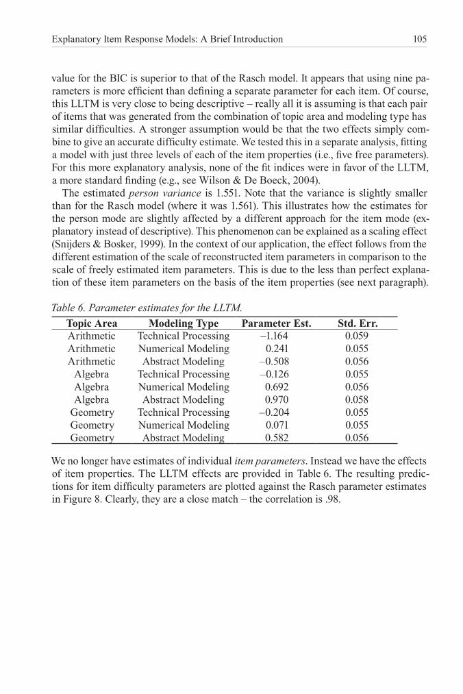
Table 6. Parameter estimates for the LLTM.Topic Area Modeling Type Parameter Est. Std. Err.Arithmetic Technical Processing –1.164 0.059Arithmetic Numerical Modeling 0.241 0.055Arithmetic Abstract Modeling –0.508 0.056

Algebra Technical Processing –0.126 0.055Algebra Numerical Modeling 0.692 0.056Algebra Abstract Modeling 0.970 0.058

Geometry Technical Processing –0.204 0.055Geometry Numerical Modeling 0.071 0.055Geometry Abstract Modeling 0.582 0.056

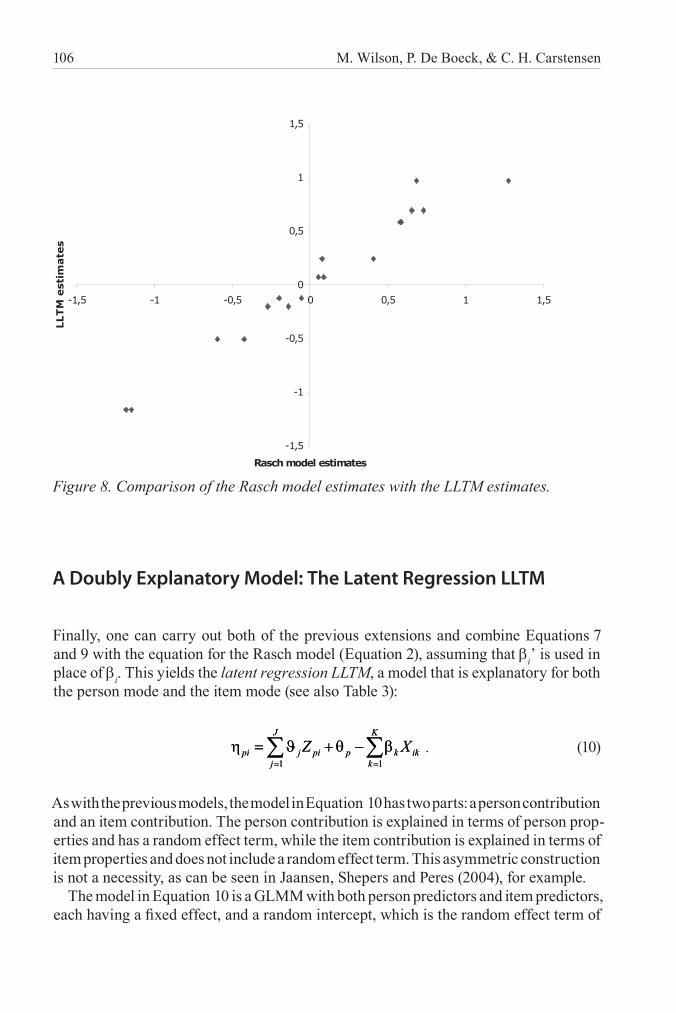
We no longer have estimates of individual item parameters. Instead we have the effects of item properties. The LLTM effects are provided in Table 6. The resulting predic-tions for item difficulty parameters are plotted against the Rasch parameter estimates in Figure 8. Clearly, they are a close match – the correlation is .98.


-1,5

-1

-0,5

0

0,5

1

1,5

-1,5 -1 -0,5 0 0,5 1 1,5

Rasch model estimates

LLTM

est

imate

s

Figure 8. Comparison of the Rasch model estimates with the LLTM estimates.

A Doubly Explanatory Model: The Latent Regression LLTM

Finally, one can carry out both of the previous extensions and combine Equations 7 and 9 with the equation for the Rasch model (Equation 2), assuming that βi’ is used in place of βi. This yields the latent regression LLTM, a model that is explanatory for both the person mode and the item mode (see also Table 3):

. (10)

As with the previous models, the model in Equation 10 has two parts: a person contribution and an item contribution. The person contribution is explained in terms of person prop-erties and has a random effect term, while the item contribution is explained in terms of item properties and does not include a random effect term. This asymmetric construction is not a necessity, as can be seen in Jaansen, Shepers and Peres (2004), for example.

The model in Equation 10 is a GLMM with both person predictors and item predictors, each having a fixed effect, and a random intercept, which is the random effect term of

1 1

J K

pi j pi p k ikj k

Z X= =

η = ϑ + θ − β∑ ∑1 1

J K

pi j pi p k ikj k

Z X= =

η = ϑ + θ − β∑ ∑


the person contribution. The previous three models in this chapter can be obtained from Equation 10. Two kinds of modifications are needed to obtain the other three models: (a) to obtain the LLTM, the Zs are omitted; and (b) to obtain the latent regression Rasch model, the Xs are restricted to just the item indicators (Xik = 1 if i = k, Xik = 0 otherwise, and K = I) so that for k = i βkXik = βi, and for k ≠ i βkXik = 0. For the Rasch model, both modifications are needed. Alternatively, these three models can be seen as being built up by adding complications to the basic building block of the Rasch model.

logitpi Xi0

Xi1,…,XiK

’i

Zp0

0

1,…,J

Zp1,…,ZpJ

p

1,…,K

piYpi

Figure 9. Graphic representation of the latent regression LLTM.

Figure 9 provides a graphic representation of the latent regression LLTM. The differ-ence between this figure and Figure 4 (the Rasch model) is that in Figure 9, for the latent regression LLTM both the contribution of each item and of each person is ex-plained through properties, item properties with a fixed effect βk, and person properties with a fixed effect ϑp, respectively. For the items, the effect of the constant predictor is β0, while for the persons, the effect of the constant predictor is a random effect which appears as θp. Note that the circle with β’i in it is not needed. A direct connection of the arrows from the Xs to ηpi is a more parsimonious but perhaps less illustrative repre-sentation. The latent regression LLTM is simply a combination of the latent regression idea with the LLTM, and this is why we call this combined model the “latent regression LLTM.” It is described theoretically in Zwinderman (1997), and Adams et al. (1997).

The fit indices for the latent regression LLTM are provided in Table 5. The goodness of fit is better than for the LLTM for the same reasons that the latent regression Rasch model had a better goodness of fit than the Rasch model. Similarly, in a comparison of the LLTM to the Rasch model, the deviance and the AIC show the latent regression LLTM to fit better than the LLTM, but the BIC shows the opposite. We will not note the specific effect estimates here, as the estimated person property effects are about the same as those obtained with the latent regression Rasch model and also the estimated


item property effects are about the same as those obtained with the LLTM.It is noteworthy that the residual person variance, after the estimated effects of

program and gender is accounted for, amounts to .663 in the latent regression LLTM, while it was .668 in the corresponding latent regression Rasch model. Again, when the model for the estimation of item effects is more flexible, the variance of the (residual) person effects is larger.

Discussion and Conclusion

The four models we have presented here serve as an introductory selection to illustrate the contrast between descriptive and explanatory models. To cover the broad variety of item response models we would need an enlargement of the perspectives. In principle the extensions can relate to the three parts of a GLMM: the random component; the link function; and the linear component.

Regarding the first two parts, the extension of the models to multicategorical data has consequences for the link function and the random component. We will not go as far as extending the models also to count data, however, which would require a loga-rithmic link and a Poisson distribution for the random component. Regarding the linear component, the extensions concern not only the type of predictors and the type of ef-fects, but also the linear nature of the component, since some extensions of these basic item response models are not GLMMs, but rather NLMMs. Examples of NLMMs are the two- and the three-parameter item response models, and the multidimensional two-parameter models. Also, the assumption of local independence can be relaxed.

For all these models, the parameters can either be descriptive or explanatory. Explanatory parameters are effects of properties or, in other words, of external vari-ables. Descriptive parameters are either random effects or fixed effects of predictors that are not really properties, but rather indicators of individual items or persons. This distinction, which is at the basis of the presentation of the four models in this chapter, can be extrapolated to include: multicategorical data (Tuerlinckx & Wang, 2004); mul-tilevel models (van den Noortgate & Paek, 2004); random (or hierarchical) item models (Janssen et al., 2004); person-by-item interaction models (incl. DIF models) (Meulders & Xie, 2004); multidimensional and 2PL models (Rijmen & Briggs, 2004); MIRID-type models (i.e., where one part of the item model predicts another part) (Smits & Moore, 2004); models involving local dependencies (Tuerlinckx & De Boeck, 2004); and mixture models (Fieuws, Spiessens & Draney, 2004).


References

Adams, R. J., Wilson, M., & Wu, M. (1997). Multilevel item response models: An approach to errors in variables regression. Journal of Educational and Behavioral Statistics, 22, 47–76.

Akaike, H. (1974). A new look at the statistical model identification. IEEE Transactions on AutomaticControl, 19, 716–723.

Bozdogan, H. (1987). Model selection for Akaike’s information criterion (AIC). Psychometrika, 53, 345–370.

Breslow, N. E., & Clayton, D. G. (1993). Approximate inference in generalized linear mixed models. Journal of the American Statistical Association, 88, 9–25.

Davidian, M., & Giltinan, D. M. (1995). Nonlinear models for repeated measurement data. London: Chapman & Hall.

De Boeck, P., & Wilson, M. (Eds.). (2004). Explanatory item response models: A generalized linear and nonlinear approach. New York: Springer-Verlag.

Embretson, S. E. (Ed.) (1985). Test Design: Developments in Psychology and Psychometrics. New York: Academic Press.

Fahrmeir, L., & Tutz, G. (2001). Multivariate statistical modeling based on generalized linear models (2nd ed.). New York: Springer.

Fieuws, S., Spiessens, B., & Draney, K. (2004) Mixture models. In P. De Boeck & M. Wilson (Eds.), Explanatory item response models: A generalized linear and nonlinear approach. New York: Springer-Verlag.

Fischer, G. H. (1973). The linear logistic test model as an instrument in educational research. Acta Psychologica, 3, 359–374.

German PISA Consortium. (2004). PISA 2003: Ergebnisse des zweiten internationalen Vergleichs (PISA 2003 Results of the second international comparison). Münster: Waxmann.

Janssen, R., Schepers, J., & Peres, D. (2004). In P. De Boeck & M. Wilson (Eds.), Explanatory item response models: A generalized linear and nonlinear approach. New York: Springer-Verlag.

Masters, G. N., Adams, R. A., & Wilson, M. (1990). Charting of student progress. In T. Husen & T. N. Postlethwaite (Eds.), International Encyclopedia of Education: Research and Studies. Supplementary Volume 2 (pp. 628–634). Oxford: Pergamon Press.

McCullagh, P., & Nelder, J. A. (1989). Generalized linear models (2nd ed.). London: Chapman & Hall.McCulloch, C. E., & Searle, S. R. (2001). Generalized, Linear, and Mixed Models. New York: Wiley.Mellenbergh, G. (1994). Generalized linear item response theory. Psychological Bulletin, 115,

300–307.Meulders, M., & Xie, Y. (2004). Person-by-item predictors. In P. De Boeck & M. Wilson (Eds.),

Explanatory item response models: A generalized linear and nonlinear approach. New York: Springer-Verlag.

Neubrand, J. & Neubrand, M. (2003). Profiles of mathematical achievement in the PISA-2000 mathematics test and the different structure of achievement in Japan and Germany. Paper presented at AERA-2003 - Annual Meeting, Chicago.

OECD (2002). PISA 2000 Technical Report. Paris: OECD.Rabe-Hesketh, S., Pickles, A., & Skrondal, A. (2001). GLLAMM Manual. Technical Report 2001/01.

Department of Biostatistics and Computing, Institute of Psychiatry, King’s College, University of London.

Rasch, G. (1960). Probabilistic models for some intelligence and attainment tests. Copenhagen, Denmark: Danish Institute for Educational Research.

Read, T. R. C., & Cressie, N.A.C. (1988). Goodness-of-fit statistics for discrete multivariate data. New York: Springer.


Rijmen, F., & Briggs, D. (2004). Multiple person dimensions and latent item predictors. In P. De Boeck, & M. Wilson (Eds.), Explanatory item response models: A generalized linear and nonlinear approach. New York: Springer-Verlag.

Schwarz, G. (1978). Estimating the dimension of a model. Annals of Statistics 6, 461–464.Smits, D. J. M., & Moore, S. (2004). Latent item predictors with fixed effects. In P. De Boeck, & M.

Wilson (Eds.), Explanatory item response models: A generalized linear and nonlinear approach. New York: Springer-Verlag.

Snijders, T., & Bosker, R. (1999). Multilevel analysis. London: Sage.Tuerlinckx, F., & De Boeck, P. (2004). Models for residual dependencies. In P. De Boeck, & M. Wilson

(Eds.), Explanatory item response models: A generalized linear and nonlinear approach. New York: Springer-Verlag.

Tuerlinckx, F., & Wang, W.-C. (2004). Models for polytomous data. In P. De Boeck & M. Wilson (Eds.), Explanatory item response models: A generalized linear and nonlinear approach. New York: Springer-Verlag.

van den Noortgate, W., & Paek, I. (2004). Person regression models. In P. De Boeck & M. Wilson (Eds.), Explanatory item response models: A generalized linear and nonlinear approach. New York: Springer-Verlag.

Verbeke, G., & Molenberghs, G. (2000). Linear mixed models for longitudinal data. New York: Springer.

Vonesh, E. F., & Chinchilli, V. M. (1997). Linear and nonlinear models for the analysis of repeated measurements. New York: Dekker.

Wald, A. (1941). Asymptotically most powerful tests of statistical hypotheses. Annals of Mathematical Statistics, 12, 1–19.

Wright, B. (1968). Sample-free test calibration and person measurement. Proceedings of the 1967 Invitational Conference on Testing. Princeton: ETS, 85–101.

Wright, B. (1977). Solving measurement problems with the Rasch model. Journal of Educational Measurement, 14, 97–116.

Wilson, M. (2005). Constructing Measures: An Item Response Modeling Approach. Mahwah, NJ: Erlbaum.

Wilson, M., & De Boeck, P. (2004). Descriptive and explanatory item response models. In P. De Boeck & M. Wilson (Eds.), Explanatory item response models: A generalized linear and nonlinear approach. New York: Springer-Verlag.

Wu, M. L., Adams, R. J., & Wilson, M. (1997). ACERConQuest: Generalized item response modeling software. Melbourne: Australian Council of Educational Research.

Zwinderman, A. H. (1997). Response models with manifest predictors. In W. J. van der Linden & Hambleton, R. K. (Eds.). Handbook of modern item response theory (pp. 245–256). New York: Springer.

Chapter 5 Explanatory Item Response Models: A Brief ... · Chapter 5 Explanatory Item Response...

Documents

Transcript of Chapter 5 Explanatory Item Response Models: A Brief ... · Chapter 5 Explanatory Item Response...