Chapter 5 Continuous Random Variables and Probability...

Chapter 5

Continuous Random Variables and

Probability Distributions

5.1 Continuous Random Variables

1

2CHAPTER 5. CONTINUOUSRANDOMVARIABLESANDPROBABILITYDISTRIBUTIONS

S tatis tics for Busi ness and Economics, 6e © 2007 Pearson Educat ion, Inc. Chap 6-4


ContinuousProbability

Distributions

Binomial

Poisson


DiscreteProbability

Distributions

Uniform

Normal

Ch. 5 Ch. 6

Figure 5.1:

Recall that a continuous random variable, , can take on any value in a given interval.

• Cumulative Distribution Function ( ) :

The cumulative distribution function, (), for a continuous random variable

expresses the probability that does not exceed the value of , as a function of x

() = ( ≤ )

• Because can take on an infinite number of possible values, its distribution is given

by a curve called a probability density curve denoted ().

Notes

1. For a continuous random variable, the probability is represented by the area under

the probability density curve.

2. The probability of any specific value of is therefore zero, i.e. ( = ) = 0 for

a continuous random variable.

3. () ≥ 04. () can be greater than one (why).

5.1. CONTINUOUS RANDOM VARIABLES 3

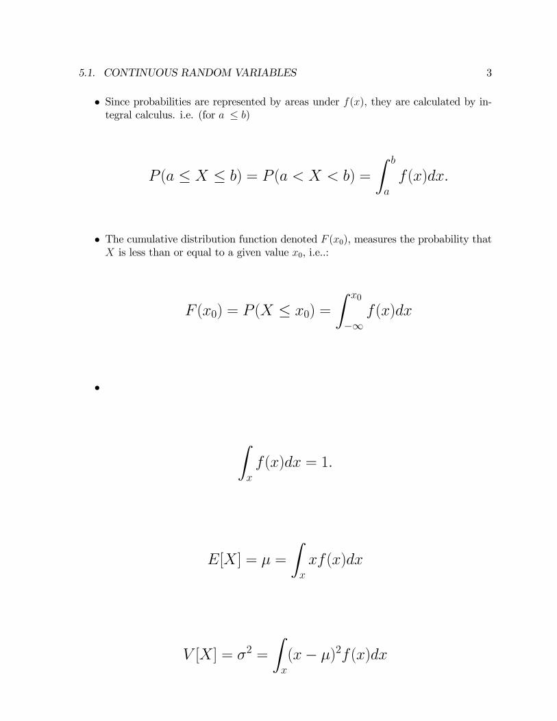
• Since probabilities are represented by areas under (), they are calculated by in-tegral calculus. i.e. (for ≤ )

( ≤ ≤ ) = ( ) =

Z

()

• The cumulative distribution function denoted (0), measures the probability that is less than or equal to a given value 0, i.e..:

(0) = ( ≤ 0) =

Z 0

−∞()

•

Z

() = 1

[] = =

Z

()

[] = 2 =

Z

(− )2()



Probability as an Area

a b x

f(x) P a x b( )=

Shaded area under the curve is the probability that X is between a and b

=

P a x b( )<<=(Note that the probability of any individual value is zero)

Figure 5.2:

5.2 The Uniform Distribution

The uniform distribution is applicable to situations in which all outcomes are equally

likely.

5.2. THE UNIFORM DISTRIBUTION 5


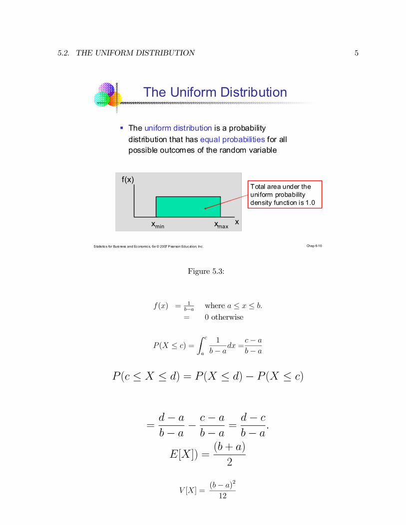
The Uniform Distribution

The uniform distribution is a probability

distribution that has equal probabilities for all possible outcomes of the random variable

xmin xmaxx

f(x)Total area under the uniform probability density function is 1.0

Figure 5.3:

() = 1− where ≤ ≤

= 0 otherwise

( ≤ ) =

Z

1

− =

−

−

( ≤ ≤ ) = ( ≤ )− ( ≤ )

=−

− − −

− =

−

−

[]) =( + )

2

[] =(− )

2

12


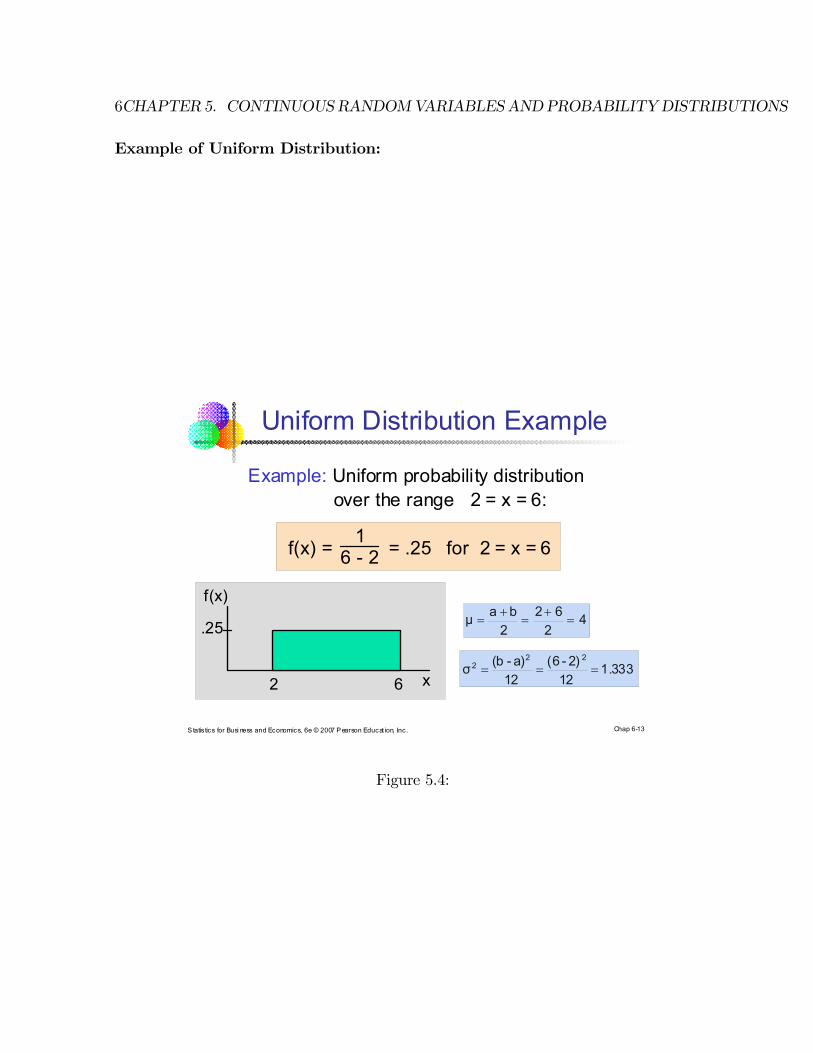
Example of Uniform Distribution:


Uniform Distribution Example

Example: Uniform probability distributionover the range 2 = x = 6:

2 6

.25

f(x) = = .25 for 2 = x = 66 - 21

x

f(x)

42

62

2

baμ

1.33312

2)-(6

12

a)-(bσ

222

Figure 5.4:

5.2. THE UNIFORM DISTRIBUTION 7

Buses are supposed to arrive in front of Dunning Hall every half hour. At the end

of the day, however, buses are equally likely to arrive at any time during any given half

hour. If you arrive at the bus stop after a hard day of attending lectures, what is the

probability that you will have to wait more than 10 minutes for the bus?

Answer

is distributed uniformly on [0,30].

() =1

30

( 10) = 1− ( 10) = 1−10− 030− 0 =

2

3

Note the expected amount of time that you will wait for a bus is:

[] =0 + 30

2= 15


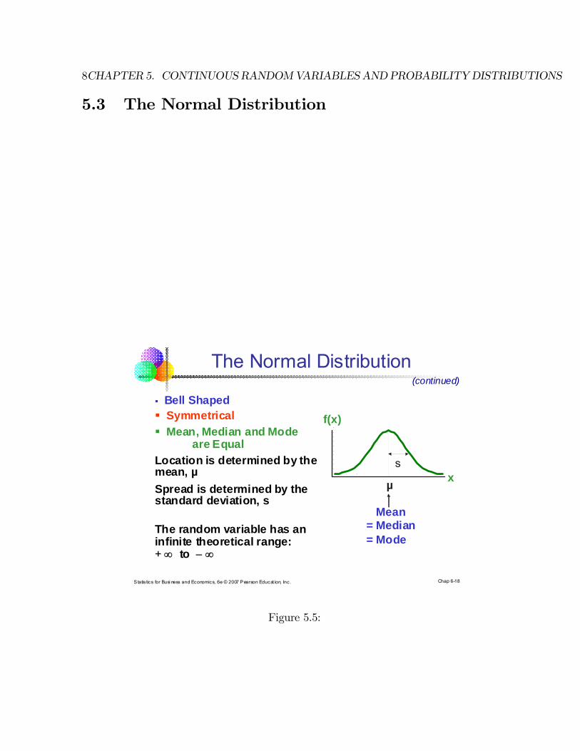
5.3 The Normal Distribution


The Normal Distribution

‘Bell Shaped’ Symmetrical

Mean, Median and Modeare Equal

Location is determined by the mean, µ

Spread is determined by the standard deviation, s

The random variable has an infinite theoretical range: + to

Mean = Median = Mode

x

f(x)

µ

s

(continued)

Figure 5.5:

5.3. THE NORMAL DISTRIBUTION 9

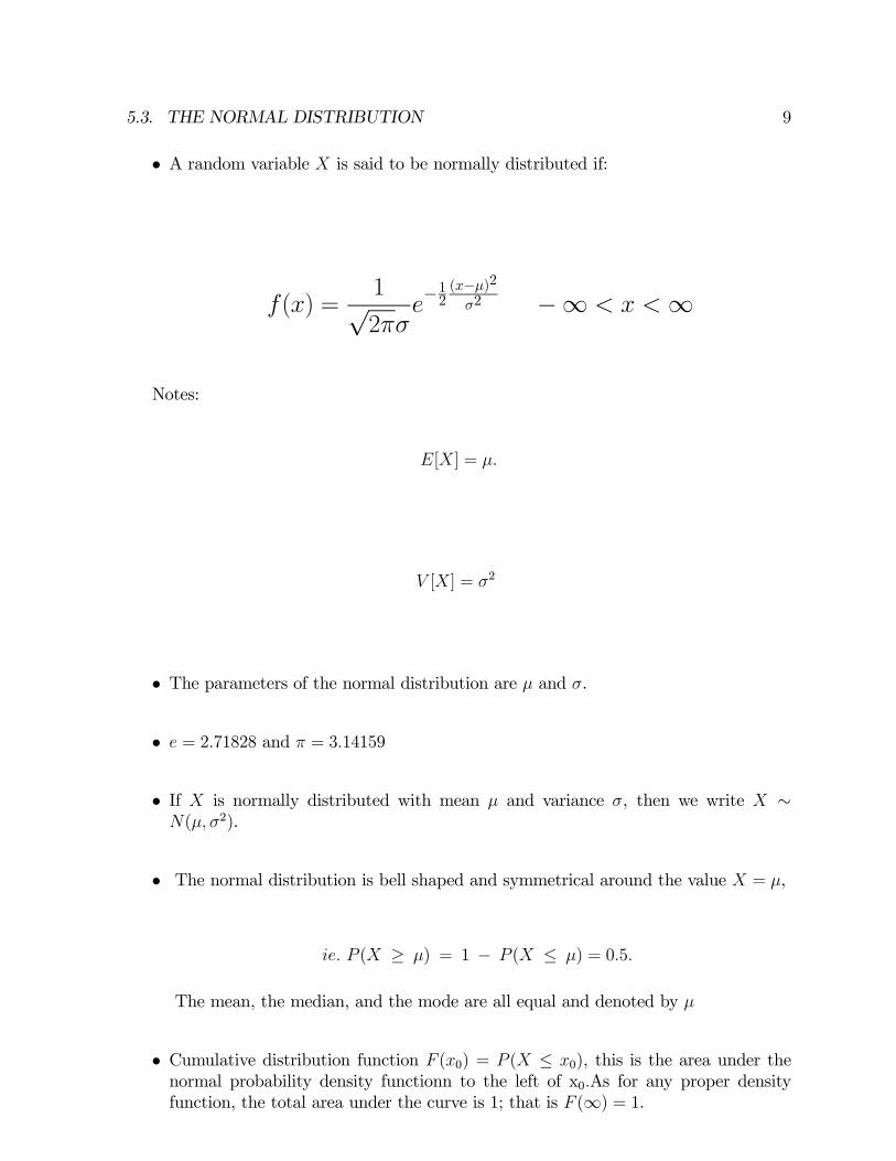
• A random variable is said to be normally distributed if:

() =1√2

−12

(−)22 −∞ ∞

Notes:

[] =

[] = 2

• The parameters of the normal distribution are and .

• = 271828 and = 314159

• If is normally distributed with mean and variance , then we write ∼( 2).

• The normal distribution is bell shaped and symmetrical around the value = ,

( ≥ ) = 1 − ( ≤ ) = 05

The mean, the median, and the mode are all equal and denoted by

• Cumulative distribution function (0) = ( ≤ 0), this is the area under the

normal probability density functionn to the left of x0As for any proper density

function, the total area under the curve is 1; that is (∞) = 1.



By varying the parameters µ and s, we obtain different normal distributions

Many Normal Distributions

Figure 5.6:

5.3. THE NORMAL DISTRIBUTION 11

Statis tics for Busi ness and Economics, 6e © 2007 Pearson Educat ion, Inc. Chap 6-21

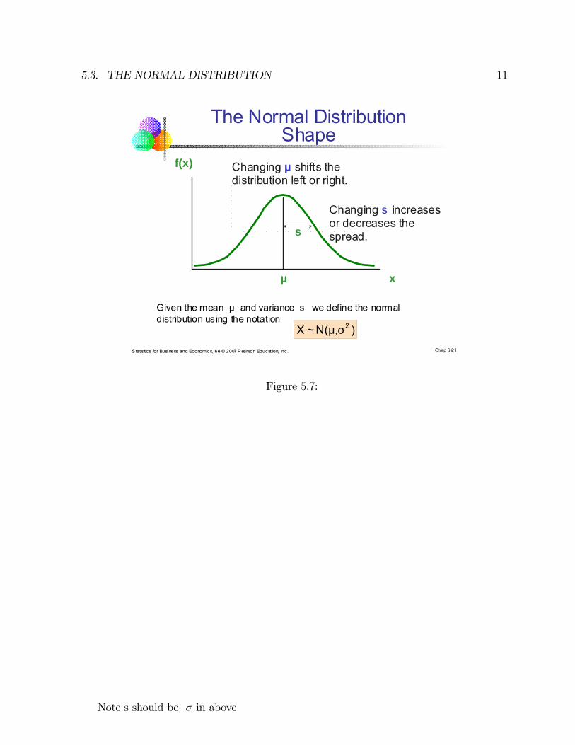
The Normal Distribution Shape

x

f(x)

µ

s

Changing µ shifts the distribution left or right.

Changing s increases or decreases the spread.

Given the mean µ and variance s we define the normal distribution using the notation

)σN(μ~X 2,

Figure 5.7:

Note s should be in above



xbµa

xbµa

xbµa

Finding Normal Probabilities (continued)

F(a)F(b)b)XP(a

a)P(XF(a)

b)P(XF(b)

Figure 5.8:

5.4. THE STANDARD NORMAL DISTRIBUTION 13

5.4 The Standard Normal Distribution


The Standardized Normal

Any normal distribution (with any mean and variance combination) can be transformed into the standardized normal distribution (Z), with mean 0 and variance 1

Need to transform X units into Z units by subtracting the mean of X and dividing by its standard deviation

1)N(0~Z ,

σ

μXZ

Z

f(Z)

0

1

Figure 5.9:

• If is normally distributed with mean = 0 and variance 2 = 1, then it is said

to have the standard normal distribution.

• A random variable with the standard normal distribution is denoted by the letter

, i.e. ∼ (0 1).


• Let (0) denote the cumulative distribution for the standard normal:

(0) = ( 0)

• It is easy to see that for 2 constants and such that

( ) = ()− ()

5.5 Calculating Areas Under the Standard Normal

Distribution

• Table 1 (page 780-781) in NCT Appendix Tables. can be used to calculate areasunder the standard normal distribution.

• Note that Table 1 gives areas between -∞ and a positive number, i.e.. ( −∞

) for some 0 (it starts at 0.5 why)

• Recall that symmetry of the normal distribution about its mean implies that ( ≥0) = 1 − ( ≤ 0).

5.5. CALCULATINGAREASUNDERTHE STANDARDNORMALDISTRIBUTION15


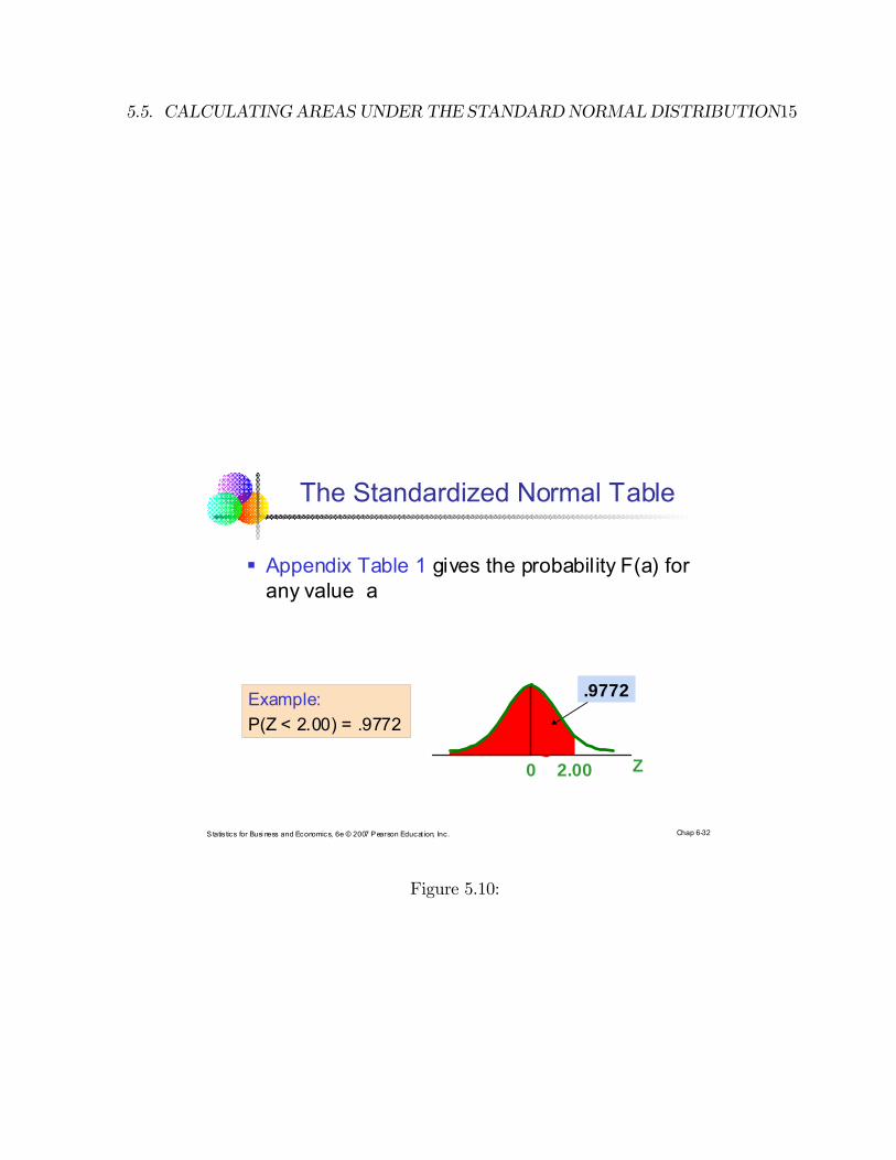
The Standardized Normal Table

Z0 2.00

.9772Example:

P(Z < 2.00) = .9772

Appendix Table 1 gives the probability F(a) for any value a

Figure 5.10:



The Standardized Normal Table

Z0-2.00

Example:

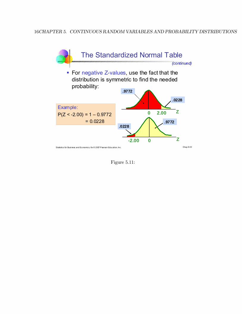
P(Z < -2.00) = 1 – 0.9772

= 0.0228

For negative Z-values, use the fact that the distribution is symmetric to find the needed probability:

Z0 2.00

.9772

.0228

.9772.0228

(continued)

Figure 5.11:

5.5. CALCULATINGAREASUNDERTHE STANDARDNORMALDISTRIBUTION17

5.5.1 Examples: of Calculating Standard Normal

• It is a good idea to draw a picture to make sure you are calculating the right area

• (0 242) = (−∞ 242) − (0) = (242) − (0) = 9922 −5000 = 4922.

• (53 242) = (−∞ 242)− (−∞ 53) = 9922− 7019 =

2903.

• ( 109) = 1− (−∞ 109) = 1− 8621 = 1379.

• ( −36) = (−∞ 36) = 6406

• (−100 196) = ( (−∞ 196)− 5)− ( (−∞ 100)− 5) =

9750− (1− 8413) = 8163.

• Find such that ( ) = 0250.

• If the area to the right of is .025,

then the area between −∞ and must be 1-.025=.975. From Table 1 we see that

• (−∞ 196) = 975, so = 196.


5.6 Linear Transformation of Normal Random Vari-

ables Theorem

• Linear combinations of normally distributed random variables are normally distrib-uted.

if 1 2 are normally distributed and

= 11 +22 + · · ·+

• is normally distributed.

• Linear combinations of normal variables are normally distributed!

• If 1 and 2 are independently normally distributed with means 1 and 2 and

variances 21 and 22, then if

= 1 +2

is normally distributed and:

[ ] = [1] +[2] = 1 + 2

• The mean of the linear combination = [ ] is equal to the sum of the individual

means 1 + 2

[ ] = [1] + [2] = 21 + 22

• The variance of the linear combination of independent variables 2 = [ ] is equal

to the sum of the individual variances 21 + 22

• So that: if ∼ ( 2) and = + then:

∼ (+22)

5.7. STANDARDIZING TRANSFORMATION 19

5.7 Standardizing Transformation

Claim: We can use the standard normal to calculate areas under any normal

curve through the use of a simple linear transformation.


An important special case of the previous results is the standardized random variable

which has a mean 0 and variance 1

Linear Functions of Variables(continued)

X

X

σ

μXZ

Figure 5.12:


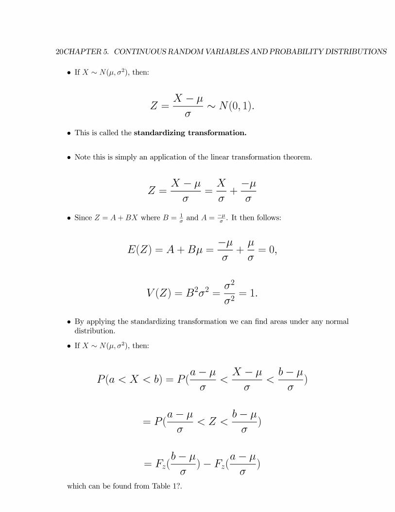
• If ∼ ( 2), then:

= −

∼ (0 1)

• This is called the standardizing transformation.

• Note this is simply an application of the linear transformation theorem.

= −

=

+−

• Since = + where = 1and = −

. It then follows:

() = + =−+

= 0

() = 22 =2

2= 1

• By applying the standardizing transformation we can find areas under any normaldistribution.

• If ∼ ( 2), then:

( ) = (−

−

−

)

= (−

−

)

= (−

)− (

−

)

which can be found from Table 1?.


Statistics for Busi ness and Economi cs, 6e © 2007 Pearson Education, Inc. Chap 6-36

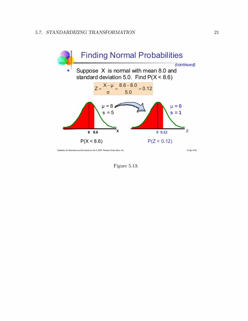
Suppose X is normal with mean 8.0 and standard deviation 5.0. Find P(X < 8.6)

Z0.120X8.68

µ = 8s = 5

µ = 0s = 1

(continued)

Finding Normal Probabilities

0.125.0

8.08.6

σ

μXZ

P(X < 8.6) P(Z < 0.12)

Figure 5.13:


5.7.1 Examples of Standardizing Normal Transformations:

Let ∼ (25 52) and find ( 24).

( 24) = ( 24− 25

5)

= ( −2) = 1− (2) = 1− 9772 = 0228

Let ∼ (1500 1002) and find (1450 1600).

(1450 1600)

= (1450− 1500

100

1600− 1500100

)

= (−5 10)

= ((10)− 5) + ((5)− 5) = 5328

Questions on Standardizing Transformation (see Examples 6.4-6.6 and try problems 6.9,6.12,



Now Find P(X > 8.6)…(continued)

Z

0.12

0Z

0.12

0.5478

0

1.000 1.0 - 0.5478 = 0.4522

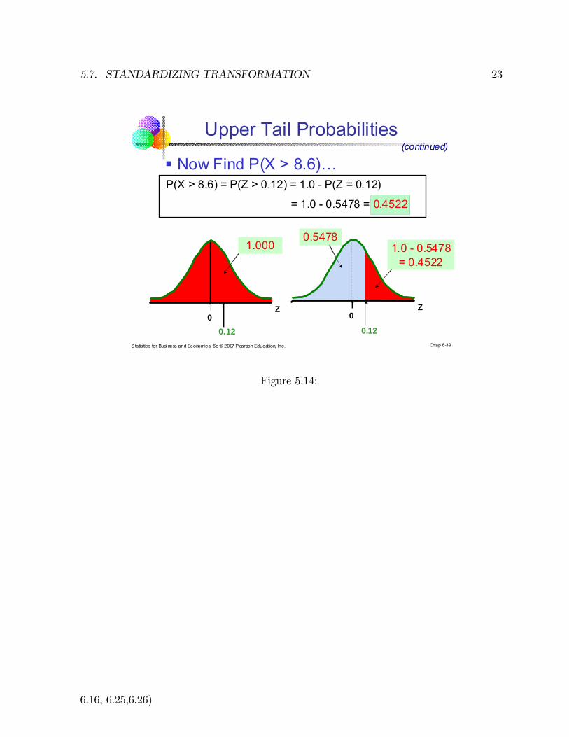
P(X > 8.6) = P(Z > 0.12) = 1.0 - P(Z = 0.12)

= 1.0 - 0.5478 = 0.4522

Upper Tail Probabilities

Figure 5.14:

6.16, 6.25,6.26)



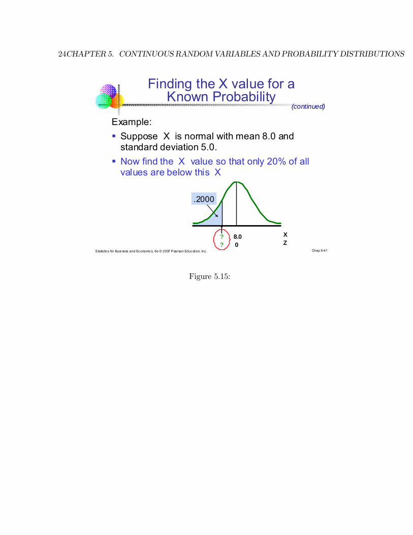
Finding the X value for a Known Probability

Example:

Suppose X is normal with mean 8.0 and standard deviation 5.0.

Now find the X value so that only 20% of all values are below this X

X? 8.0

.2000

Z? 0

(continued)

Figure 5.15:



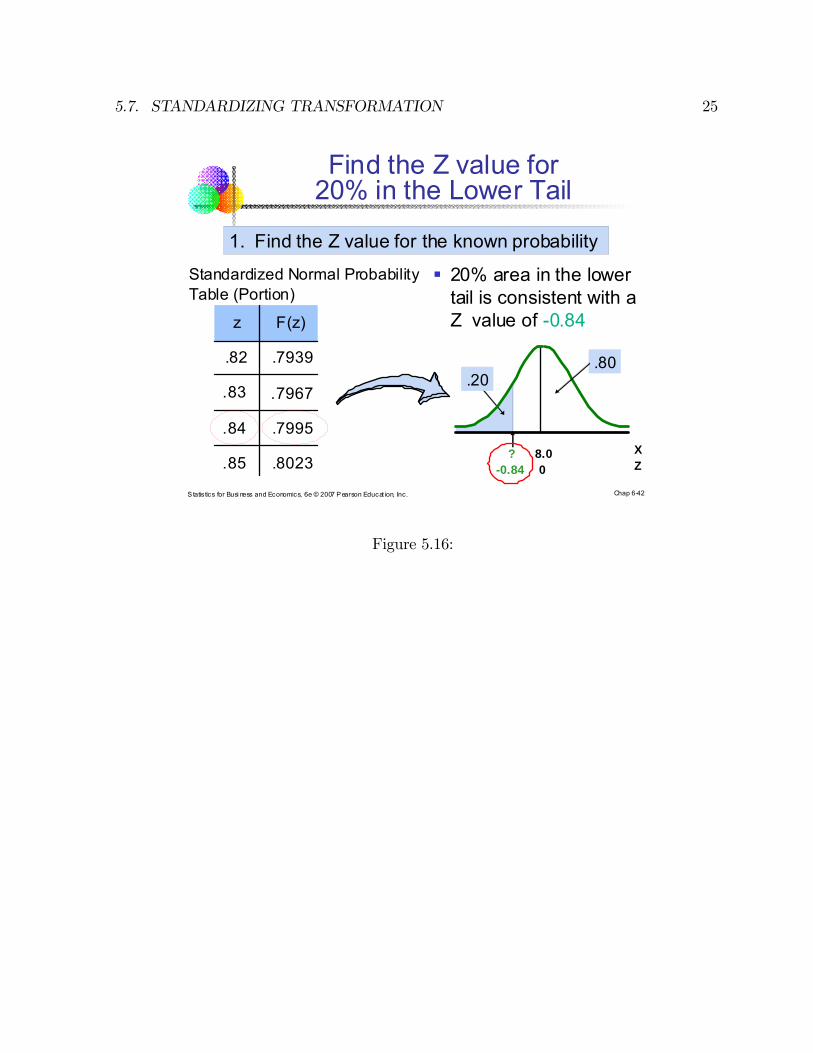
Find the Z value for 20% in the Lower Tail

20% area in the lower tail is consistent with a Z value of -0.84

Standardized Normal Probability Table (Portion)

X? 8.0

.20

Z-0.84 0

1. Find the Z value for the known probability

z F(z)

.82 .7939

.83 .7967

.84 .7995

.85 .8023

.80

Figure 5.16:



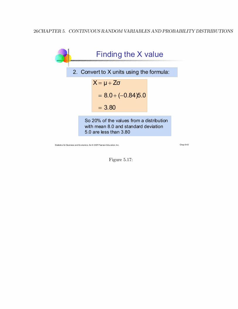
2. Convert to X units using the formula:

Finding the X value

80.3

0.5)84.0(0.8

ZσμX

So 20% of the values from a distribution with mean 8.0 and standard deviation 5.0 are less than 3.80

Figure 5.17:

5.8. NORMALDISTRIBUTIONAPPROXIMATIONFORBINOMIALDISTRIBUTION27

5.8 Normal Distribution Approximation for Binomial

Distribution

• Let = the number of sucessesin independent trilas with probability of success

• As gets big the binomial distribution converges into a normal distribution

• This is an example of the Central Limit Theorem

• If is large and is close to .5 then we can use the normal distribution to get a

good approximation to the binomial distribution by setting

[] = = and [] = 2 = (1− )



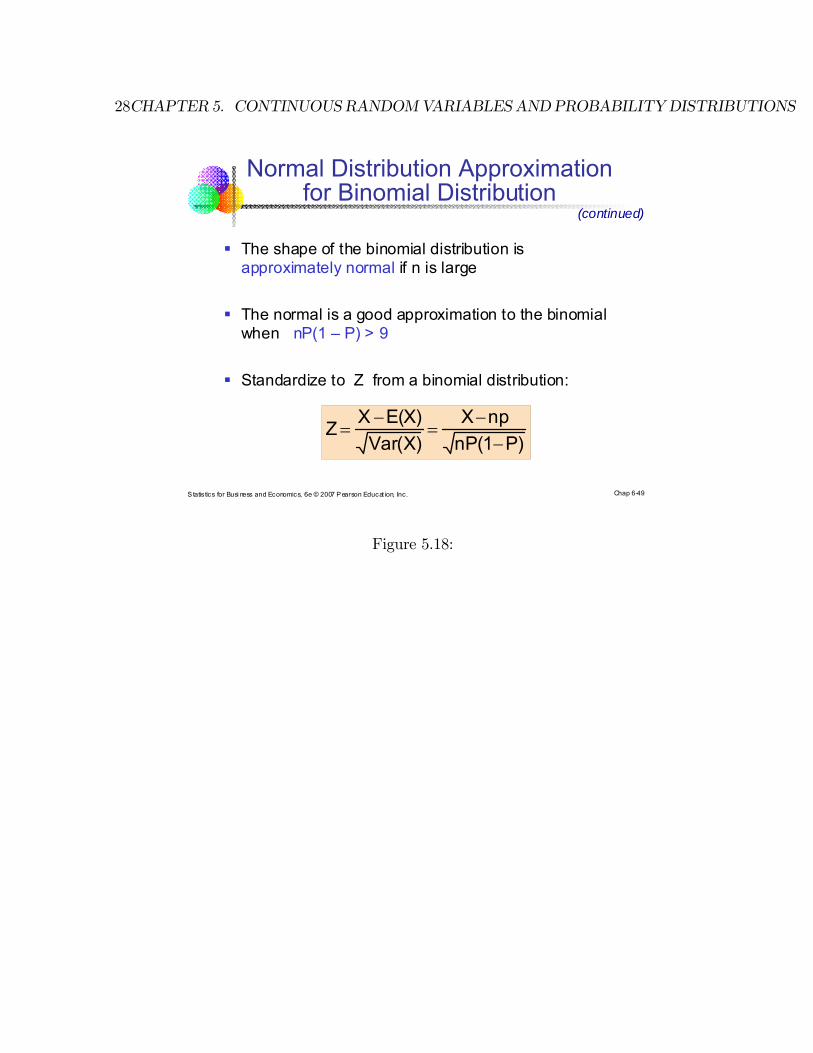
Normal Distribution Approximation for Binomial Distribution

The shape of the binomial distribution is approximately normal if n is large

The normal is a good approximation to the binomial when nP(1 – P) > 9

Standardize to Z from a binomial distribution:

(continued)

P)nP(1

npX

Var(X)

E(X)XZ

Figure 5.18:

5.9. CONTINUITY CORRECTION FOR THE BINOMIAL 29

• A general guideline is the normal distribution approximates the binomial distribu-tion well whenever: (1− ) ≥ 9.

• The equation for the standardized binomial variable (where is the number of

successes) is:

= −[]p []

= − p(1− )

5.9 Continuity Correction for the Binomial

• We can improve the accuracy of the approximation by applying acorrection forcontinuity.

• This adjusts the probability to account for the fact that we are approximating adiscrete distribution with a continuous one.

• The rule is to subtract .5 from the lower value of the number of successes, and add

.5 to the upper value.

i.e. we approximate ( = ) by

(− 5 + 5)

• and approximate ( ≤ ≤ ) by

( ≤ ≤ ) ∼= (− 05− p

(1− )≤ ≤ + 05− p

(1− ))

• The text NCT, makes a distinction as to when the continuity corrections can be ap-plied if (5 (1−) 9)–this is really not necessary since continuity corrections

will always improve accuracy

• In some cases the difference with or without corrections is minimal ((1− ) 9)


5.10 Example of Continuity Correction for Binomial

Approximation

• Suppose 36% of a companies workers belong to unions and the personnel manager

samples 100 employees. We are asked to find the probability that the number of

unionized workers in the sample is between 24 and 42 inclusive, so = 36 = 100

5.11 Exact Probability Using the Binomial Distribu-

tion

• Using the binomial distribution which gives the exact probability

(24 ≤ ≤ 42) =42X

=24

µ100

¶(36)(64)100−

= 9074

5.12 Normal Approximation without Continuity Cor-

rection

• Without continuity correction (an approximation):

= = 36× 100 = 36

=p(1− ) =

p(100× 36× 64) = 48

(24 ≤ ≤ 42) ≈ (24− 3648

≤ ≤ 42− 3648

)

≈ (−25 ≤ ≤ 125) = 8882

5.13 Normal Approximation with Continuity Correc-

tion: A Better Aproximation

(24− 5 ≤ ≤ 42 + 5) = (235 ≤ ≤ 425)= (

235− 3648

≤ ≤ 425− 3648

)

≈ (−260 ≤ ≤ 135) = 9068

5.14. QUESTIONS: 31

5.14 QUESTIONS:

1. 6.29, 6.32, 6.33, 6.50, 6.59,

2. Suppose a golfer is on the first tee of the Kingston Golf and Country Club. His first

shot is taken with a driver and his second shot is taken with a three iron.

Let 1 be the length with his driver and 2 be the length with his three iron.

Assume that 1 and 2 are independently normally distributed, with: and

1 = 200 yards, 1 = 20 yards

2 = 150 yards, 2 = 10 yards

What is the probability that his first two shots travel more than 400 yards?

3. The distance a discus thrower can throw a discus is normally distributed with mean

100 meters, and variance 25 meters. If his throws are independent, what is the probability

that 2 out of 3 throws travel more than 105 meters?

• Skip the exponential Distribution

5.15 Jointly Distributed Continuous Random Vari-

ables

• Let 1 2 be continuous random variables

• The joint cumulative distribution function (1 2 ) defines the prob-

ability that simulataneously 1 is less than 12 is less than 2, and so on:

(1 2 ) = (1 1 ∩2 2 ∩ )

• The marginal distribution functions are: (1) (2) ()• If 12 are independent:

(1 2 ) = (1)× (2)× × ()

5.15.1 Covariance

• As with discrete random variables, we can define covariances for continuous randomvariables:

[ ] = [ − ][ − ]

= [ ]−

• If and are independent then

[ ] = 0⇒ [ ] =


5.15.2 Correlation

• Let 1 2 be continuous random variables, then the correlation between

and is

= [ ] =[ ]

5.15.3 Sum of Random Variables

• Let 12 be continuous random variables with means 1 2 and

variances 21 22

2 then

[1 +2 + + ] = 1 + 2 + +

and if 12 are independent (or have zero covariance—a weaker condition)

the variance of the sum of contiuous random variables

[1 +2 + + ] = 21 + 22 + + 2

and if the covariances areNOT zero, the variance of the sum of continuous random

variables is:

[1 +2 + + ] = 21 + 22 + + 2 + 2

−1X=1

X=+1

[]

5.15.4 Differences Between A Pair of Random Variables (Spe-

cial case: = 2)

• Let and be two contiuous random variables

[ − ] = −

• If and are independent (or have zero covariance–a weaker condition)

[ − ] = 2 + 2

• If covariance of and is NOT zero then

[ − ] = 2 + 2 − 2[ ]

5.15.5 Linear Combinations of Random Variables

• Let and be two contiuous random variables, and are two constants

= +

• = [ ] = +

•2 = [ ] = 22 + 22 + 2[ ]

= 22 + 22 + 2[ ]

• Exercise 6.39-6.45

5.15. JOINTLY DISTRIBUTED CONTINUOUS RANDOM VARIABLES 33


Example

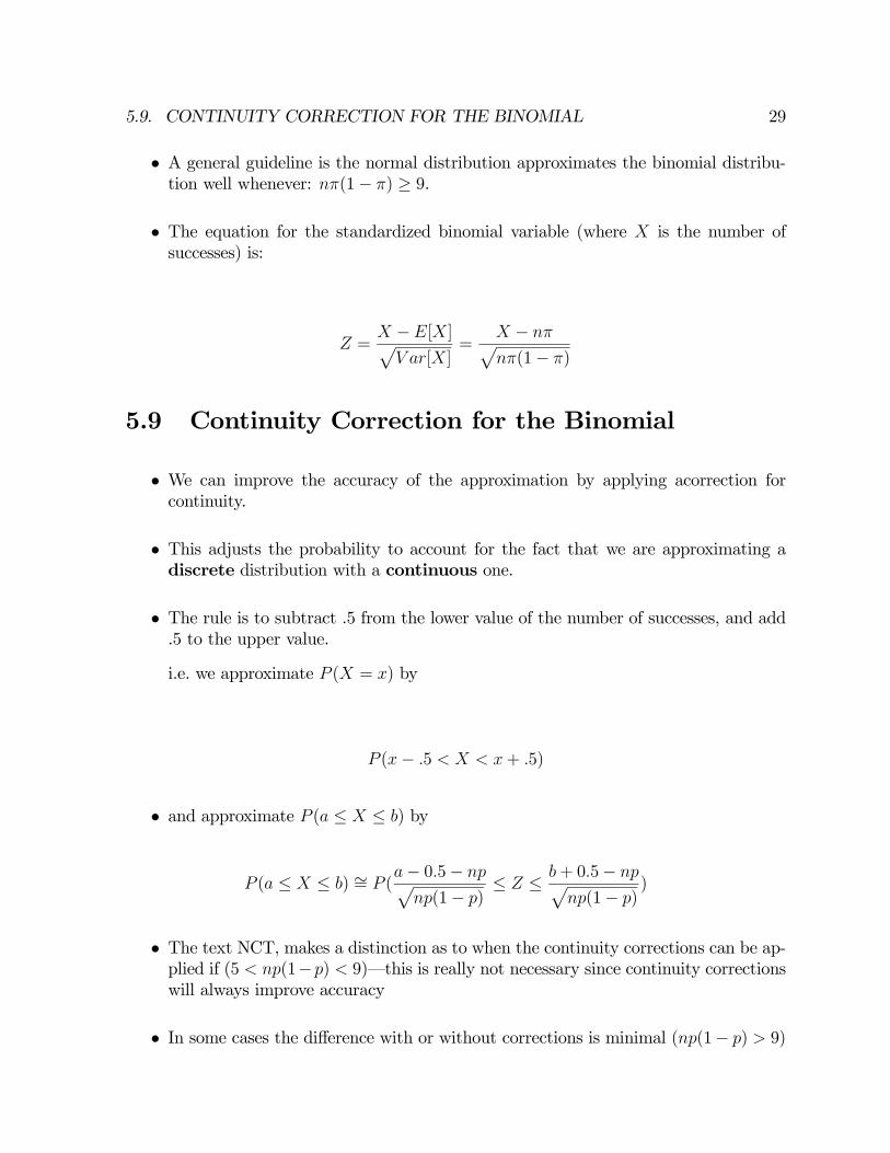
Two tasks must be performed by the same worker.

X = minutes to complete task 1; µx = 20, sx = 5

Y = minutes to complete task 2; µy = 20, sy = 5

X and Y are normally distributed and independent

What is the mean and standard deviation of the time to complete both tasks?

Figure 5.19:


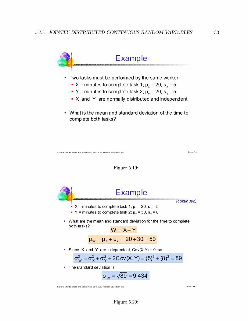
Example

X = minutes to complete task 1; µx = 20, sx = 5

Y = minutes to complete task 2; µy = 30, sy = 8

What are the mean and standard deviation for the time to complete both tasks?

Since X and Y are independent, Cov(X,Y) = 0, so

The standard deviation is

(continued)

YXW

503020μμμ YXW

89(8)(5) Y)2Cov(X,σσσ 222Y

2X

2W

9.43489σW

Figure 5.20:

Chapter 5 Continuous Random Variables and Probability...

Documents

Transcript of Chapter 5 Continuous Random Variables and Probability...