Chapter 4The Two-Sample Location Problem

.continuous are onsdistributiBoth A3.

t.independenmutually are s' and s' A2.

~,...,,

~,...,, A1.

sAssumption

population treatment thefrom - ,...,,

population

control thefrom sample control a ,...,,

:samples 2 involvesstudy A

21

21

21

21

YX

GYYY

FXXX

YYY

XXX

iid

n

iid

m

n

m

0:

toreduces hypothesis null The

or

)()(

:modelshift -location The

)()(:

hypothesis null Original

0

0

H

H

XY

ttFtG

ttGtFH

d

o

§4.1 The Wilcoxon-Mann-Whitney Rank Sum Test for the Location-Shift Model

Order the combined X-sample and Y-sample in an ascending order.

Let S1 = the rank of Y1

S2 = the rank of Y2

. ….

Sn = the rank of Yn

in the combined sample of m+n.

wnmnWwW

wnmnW

wW

H

SWn

jj

)1(or 0

)1( 0

0

:

RuleRejection

statisticTest

1

1

A.6 Table from )Pr(

where

wW

))1(

2

1Pr())1(

2

1Pr(

df same thehas )1(2

1 and )1(

2

1

)1()1( As

ondistributi same thehas and ',Under

etc. ' 1 If

) ofn (reflectio 1'

''

: Proof

ondistributi same thehas )1(2

1 and )1(

2

1-

2

)1(about ddistributelly symmetrica is

'

'

0

n

1

kWNnkNnW

WNnNnW

WNnSNW

WWH

NSS

SSNS

SW

wmnnnmnW

mnnW

SS

SS

SiS

ii

iii

ii

}2

)1(,...,

2

)1({ that Note

)Pr(

)2

)1(

2

)1(Pr(

)2

)1(

2

)1(Pr() )1(Pr(

nnnm

nnW

wW

wNn

WNn

wNnNn

WwnmnW

Sampling from a finite PopualtionSuppose a population consists of N numbers

factor correction population finite the1

1 where

1

)(

... )E(

.

average sample drawn with is size of sample random simpleA

.,...,,

2

1

22

2

^21

21

N

nN

vN

N

nN

nvVar

N

vvvv

v

n

vvv

pop

N

iipop

popn

popN

n

n

N

0

2

0

under

12

)1()(

2

)1()(

12

)1(

112

)1)(1(

1)(

2

1)E(

N}{1,2,..., fromdrawn sample random simple a ofmean sample

likely.equally are ranks

possible N

all , Under ranks. of average theis that Note

Hmnnm

WVar

mnnWE

n

Nm

N

nN

n

NN

N

nN

nn

WVar

N

n

W

n

W

mnNY

nHY

n

W

pop

pop

Large Sample Tests

tests.sample large do toused becan This

.under and as

)1,0(

12)1(

}2

)1({

0

*

Hn

Nmnmn

nmnW

W d

Table 4.1 Tritiated Water Diffusion Across Human Chorioamnion

Pd (10-4 cm/s)

At Term 12-26 weeks Gestational Age

0.80 1.15

0.83 0.88

1.89 0.90

1.04 0.74

1.45 1.21

1.38

1.91

1.64

0.73

1.46

Example 4.1: Water Transfer in Placental Membrane. The data in Table 4.1are a portion of the data obtained by Lloyd et al. (1969). Among other things, these authors investigated whether there is a difference in the transfer of tritiated water (water containing tritium, a radioactive isotope of hydrogen) across the tissue layers in the term human chorioamnion (a placental membrane) and in the human chorioamnion between 3 to 6 months gestation age. The objective measure used was the permeability constant Pd of the human chorioamnion to water. The tissues used for the study were obtained within 5 min of delivery from the placentas of healthy, uncomplicated pregnancies in the following gestation age categories: (a) between 12 and 26 weeks following termination of pregnancy via abdominal hysterotomy (surgical incision of the uterus) for psychiatric indications; and (b) term, uncomplicated vaginal deliveries. Tissues from ten term pregnancies and five terminal pregnancies were used in the experiment. Table 4.1 gives the average permeability constant (in units of 10-4 cm/s) for six measurements on each of the 15 tissues in the study.

In this example, the alternative of interest is greater permeability of the human chorioamnion for the term pregnancy. Thus, if we let X correspond to the Pd values of tissues from term pregnancies and Y to the Pd values of tissues from terminated pregnancies, we perform test (4.5), which is designed to detect the alternative Δ < 0.

For purpose of illustration we choose α to be 0.082. From Table A.6 we find w0.082 = 52. Now we list the combined sample in increasing order to facilitate the joint ranking. The ranks are given in parentheses

X Y X X Y Y X Y

0.73 0.74 0.80 0.83 0.88 0.90 1.04 1.15

(1) (2) (3) (4) (5) (6) (7) (8)

Y X X X X X X

1.21 1.38 1.45 1.46 1.64 1.89 1.91

(9) (10) (11) (12) (13) (14) (15)

We see that the Y-ranks are 2,5,6,8,9 and thus

W = 2+5+6+8+9 = 30.

.28W-1)mn(n Wif HReject 0

1600150014001300120011001000900800700

8

7

6

5

4

3

2

1

0

Xdat

Fre

qu

en

cy

X-data

11001000900800700600500400300200

9

8

7

6

5

4

3

2

1

0

Ydat

Fre

qu

en

cy

Y-data

Control SST

1042 (13) 874 (9)

1617 (23) 389 (2)

1180 (18) 612 (4)

973 (12) 798 (7)

1552 (22) 1152 (17)

1251 (19) 893 (10)

1151 (16) 541 (3)

1511 (21) 741 (6)

728 (5) 1064 (14)

1079 (15) 862 (8)

951 (11) 213 (1)

1319 (20)

Table 4.2 Alcohol Intake for 1 Year (cl of Pure Alcohol)

Example 4.2 : Alcohol Intakes. Eriksen, Bjornstad, and Gotestam (1986) studied a social skills training program for alcoholics. Twenty-four “alcohol-dependent” male inpatients at an alcohol treatment center were randomly assigned to two groups. The control group patients were given a traditional treatment program. The treatment group patients were given the traditional treatment program plus a class in social skills training (SST). After being discharged from the program, each patient reported – in 2-week intervals – the quantity of alcohol consumed, the number of days prior to his first drink, the number of sober days, the days worked, the times admitted to an institution, and the nights slept at home. Reports were verified by other sources (wives or family members). (Such data can be unreliable!) One patient in the SST group, discovered to be an opiate addict, disappeared after discharge and submitted no reports. The remaining 23 patients reported faithfully for a year. The results for alcohol intake are given in Table 4.2. The ranks in the joint ranking of the 23 observations are given in parentheses in Table 4.2.

.14.3264

13281

}12

)11112)(11(12{

2)11112(11

81W

21

*

To test H0 vs the alternative that the SST group tends to have lower alcohol intakes, we need to test H0 : Δ = 0 vs H2 : Δ < 0. Suppose, for example, we choose α = 0.05. Then z0.05 = 1.645 and the normal approximation given by the display (4.11) is Reject H0 if W* -1.645; otherwise do not reject.

From Table 4.2, we find the sum of the SST ranks is W = 9+2+4+7+17+10+3+6+14+8+1=81

Then from equation (4.9) we obtain

).Pr( , , where

)21

)(1(12

)(

2

)1(

otherwise. 0

if 1),( where

),(

Statistic Whitney U-Mann The

2

2

1 1

YXnmNcNm

cc

zzN

nnUW

YXYX

YXU

jiji

m

i

n

jji

ionDeterminat Size Sample

2

)1(

So,

),(W

sample. combined in the Y ofrank theis Wwhere

...

.}{X torelativerank Y of sum

of #),(

....Ylet WLG,

),(

1

1j

ji

1

n1iij

21

1 1

nnUjUW

jYX

WWW

YXYX

YY

YXU

n

i

n

iji

n

jiji

n

m

i

n

jji

.])0()1

12([

)()Power( ,0: If

)population (the ~,

ofdensity theis )0( where

])0()1

12[( where

)()Power(

0: vs0:

*21

1

21

21*

*21

10

zfmn

mnA

AH

XFXX

XXf

zfmn

mnA

A

HH

F

F

iid

F

F

test sum rank the ofPower

645.1-

645.166-)Power(

261.1ˆ )0(

)2,0(~X ofdensity theis f

).,Normal(~X Suppose

89.79124S , 91.739

8.68168,55.1167

645.1)0()Power(

test.5% for thepower theEvaluate

Data. Intake Alcohol :e.g

1.261233

221

221*

221

*

2

2Y

2

*2/1

2411*12*12

f

NX

Y

SX

f

X

X

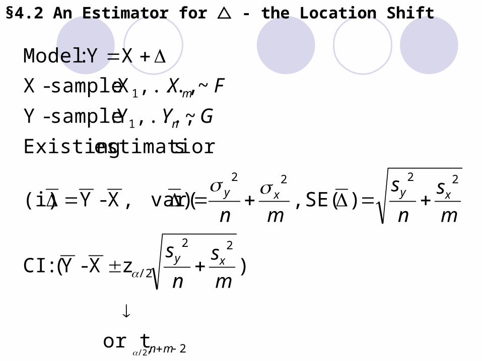
§4.2 An Estimator for - the Location Shift

2,

22

/2

2222

1

1

/2or t

)zX-Y( :CI

)SE( ,) var(,X-Y (i)

sestimatior Existing

~,...,Y : sample-Y

~,...,X :sample-X

XY :Model

mn

xy

xyxy

n

m

m

s

n

s

m

s

n

s

mn

GY

FX

jiXX

jiYY

ji

ji

,2

ofmedian

,2

ofmedian

ˆˆˆ̂

ly.respective sample-Y and sample-X of averages

Walsh on the basedestimator median thebe ˆ and ˆLet

. -

ly.respective spopulation Y & Xmedian thebe & Let ii)(

12

21

12

21

).ˆ̂

(zˆ̂

for CI eapproximatAn

22

)ˆ(SE)ˆ(SE )ˆ̂

SE(

)ˆvar()ˆ var(

)ˆˆvar()ˆ̂

var(

Error. Standard

averages. Walsh ordered on the based

,for CI -1 a be ),(

,for CI -1 a be ),(Let

/2

2

2/

11

2

2/

22

12

22

12

12

2222L

1111L

12

SE

zzLULU

U

U

.ˆY of half2

)ˆU(

rejected. be hardest to theisshift -zerofor

H when 2

)ˆ U(make should ,ˆsay , of choice goodA

.otherwise0

0X if1),(

),()Let U(

on.dsitributi same thefrom come

-,...,Y & ,...,X

modelshift location Under the

:ionjustificatA

},...,1;,...,1 ,median{Yˆ

estimator newA

j

0

i

1i

n

1j

11

j

i

jji

m

ji

nm

i

Xmn

mn

YYX

YX

YX

njmiX

j}i,|X-{Ymedian theˆ

ˆ of halfother an and ˆ of half

0ˆ of half

1),( of half2

)ˆU(

rejected. be hardest to theis 0:H the

and 2

)ˆ U(make should ,ˆsay , of choice reasonableA

)()(

.otherwise0

0X if1),(

),()U(

on.distributi same thefrom come ,...,Y & ,..,X

modelshift -location under theion justificatA

ij

2mn

2mn

0

22)1(

i

1 1

11

ijij

ji

ji

mnnn

jji

m

i

n

jji

nm

XYXY

YX

YX

mn

mn

WEUE

YYX

YX

YX

21

21

21

2

22

1210

(j)j

(i)i

(n)(1)(m)(1)

11

0

0

)Pr(0

)1(

)2

1()(

S

sample combined in the Y ofrank theS

sample combined in the X ofrank theRLet

Y...Y ;X...X

samples Y and Xorder ),ˆSE( derive To

ˆ :parameter meaningful moreA

)P(Xparameter naturalA

YX

nm

mRmiR

mn

U

Y

m

ii

0

/2

201

210

/2

0

0

0

201

210

201

2102

zˆzˆ

is for CI -1A

n )ˆSE(

.m,n as )1,0()ˆ(

n

that proved)1967(Sen

& of average weighted

n

s

nm

mSnS

nm

mn

n

s

Ns

SSnm

mSnSS

d

2

22

1201 )1(

)2

1()(

mn

nSnjS

S

n

jj

enough. strongnot

is H rejecting of evidence theSo, ).(0,0.56257 Now

. toscorrespond 0:H

)(0,0.56257)0.18891.39(0,0.3)ˆ(0,

0.9180.082-1-1 :for band confidencelower A

test.CIbetween ipRelationsh

)(0.02,0.58 CI 95% 015.0S 171.0

3.0ˆ

Wolfe&Hollander of 4.1 eg ofon continuati :eg

021

21

0

mnnS

201

210

5*1015

201

210

mSz

S

§4.3 CIs for based on the Mann-Whitney Statistic

Ys? from subtract Why :Q

.otherwise0

0X if1),(

),(Let U

ion.justificatA

(4.3.1) )U,(U

is for CI -1 aThen

.12

)12(CSet

n.1,...,j m;1,...,ifor Y ordered be ...Let U

i

1i

n

1j

)C-1(mn)(C

2/

j)((1)

jji

m

ji

imn

YYX

YX

Wnmn

XU

.1

))1(Pr(1

)Pr()1)1(Pr(

)C-1mnPr()CPr(

)UPr()UPr(

)UPr(U

(*) 1 U

mn,t1any For :factA

22/

2/2/

)(C)C-1(mn

)C-1(mn)(C

(t)

WnmnW

WWWnmnW

UU

tmnU

1

1

))1(Pr(1

)Pr()1)1(Pr(

)Pr()1Pr(

)1Pr()Pr(

)1Pr()1Pr(

)Pr()Pr(

)Pr()Pr(

)Pr(

111

.,...,1;,...,1,Y ordered are ...

Test SumRank on the based for CIs

22

22/

2/2/

2/2)1(

2/2)1(

)()(

)()(

)()(

2/2)1(

2/2)1(

j)()1(

WnmnW

WWWnmnW

WUWmnU

CmnUCU

CmnUtmnU

UU

UU

UU

W

WmnmnCmnt

njmiXUU

nnnn

Ct

Ct

tC

nn

nn

imn

Large Sample CIs:

For large m & n, approximate Cα

(4.3.1).equation in

2

2/1

12)1(

2/ nmmnz

mnC

(4.3.1).equation in

2

2/1

12)1(

2/ nmmnz

mnC

§4.4 Relative Efficiencies

test.- tsample one themeans tand

rank test signed themeans T where

),e(T

as same theisIt

.})({12)te(W,

istest - t the test toSumRank theof efficiency relative The2

)1()1(

t

test- tsample Two

1

1

2222

222

112

t

dxxf

nm

snsms

s

XY

F

yxp

nmp

§4.5 Kolmogorov-Smirnov test for general differences

Will abandon the location-shift model

Y = X +

Assume no particular relationship between F, the df of X-population, and G, the df of Y-population.

Still assume X and Y both are continuous r.v.s, and independence both within a sample and between the samples.

t.oneleast at for )()(:H

vs

),(- t )()(:

1

0

tGtF

tGtFH

samples. Y & X

combined ordered theare n,mN ,... where

|)(G)(|max

|)(G)(|max

)H sided-2(for statisticTest

n. &m ofdivisor common greatest d

Y of no.)(G

X of no.)(FLet

)()1(

)(n)(m,...,1

nm

1

in

im

N

iiNid

mn

tdmn

ZZ

ZZF

ttFJ

n

tt

m

tt

jNmj

Nj

jNn

jNm

Nj

jj

jj

jNm

jNn

Nj

jnNmn

jmNmn

Nj

jnjmNjd

mn

j

Z

jZZ

ZZ

ZGZF

ZGZFJ

...max

}...{}...{maxJ

So,

...}X of {# and

}Y of {#}X of {# As

}Y of {#}X of {#max

)()(max

)()(max

21,...,1d

N

2121,...,1d

N

21)(

)()(

)()(,...,1d

N

)()(,...,1d

N

)()(,...,1

3 )1,1,,( (0,0,0,1)

2 )1,,,( (0,0,1,1)

2 )1,,,( (0,1,1,1)

3 )1,,(0, (1,1,1,1)

J )(G )(F Meshings

1,d 3,n 1,mFor . prob havingeach and likely,equally

are sY' and sX' of meshings n

N possible all ,HUnder

ties)(no Hunder J ofon distributi The

|}||,...,max{|J

then

]...[

otherwise0

nobservatio Xan is Zif1

tie,no is thereIf

32

31

32

32

31

32

31

31

32

31

31

n

N1

0

0

1

j1

(i)i

YYYX

YYXY

YXYY

XYYY

ZZ

SS

S

ii

NdN

Njm

j

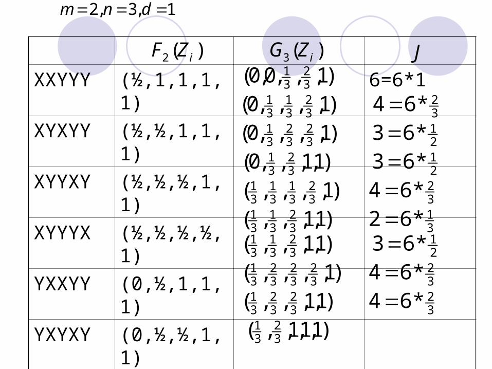
1,3,2 dnm

XXYYY (½,1,1,1,1) 6=6*1

XYXYY (½,½,1,1,1)

XYYXY (½,½,½,1,1)

XYYYX (½,½,½,½,1)

YXXYY (0,½,1,1,1)

YXYXY (0,½,½,1,1)

YXYYX (0,½,½,½,1)

YYXXY (0,0,½,1,1)

YYXYX (0,0,½,½,1)

YYYXX (0,0,0,½,1) 6=6*1

)(2 iZF )(3 iZG J)1,,,0,0( 3

231

)1,,,,0( 32

31

31

)1,,,,0( 32

32

31

)1,1,,,0( 32

31

)1,,,,( 32

31

31

31

)1,1,,,( 32

31

31

)1,1,,,( 32

31

31

)1,1,,,( 32

32

31

)1,,,,( 32

32

32

31

)1,1,1,,( 32

31

32*64

21*63

21*63

32*64

31*62 21*63

32*64

32*64

J 2 3 4 6

Prob101

103

104

102

)jPr(J wherejJ if

),()(:H vs)()(:HReject

:procedureTest

n.m assume ,generality of lossWithout

10 xGxFxGxF

Example 5.4: Effect of Feedback on Salivation Rate

The effect of enabling a subject to hear himself salivate while trying to increase or decrease his salivary rate has been studied by Delse and Feather (1968). Two groups of subjects were told to attempt to increase their salivary rates upon observing a light to the left, and decrease their salivary rates upon observing a light to the right. The apparatus for collecting and recording the amounts of saliva was described by Delse and Feather (1968) and also Feather and Wells (1966). Members of the feedback group received a 0.2-s, 1000-cps tone for each drop collected, whereas members of the no-feedback group did not receive any indication of their salivary rates. Table 5.7 gives differences of the form mean number of drops over 13 increase signals- mean number of drops over 13 decrease signals for the feedback group and the no-feedback group, each group consisting of 10 subjects.

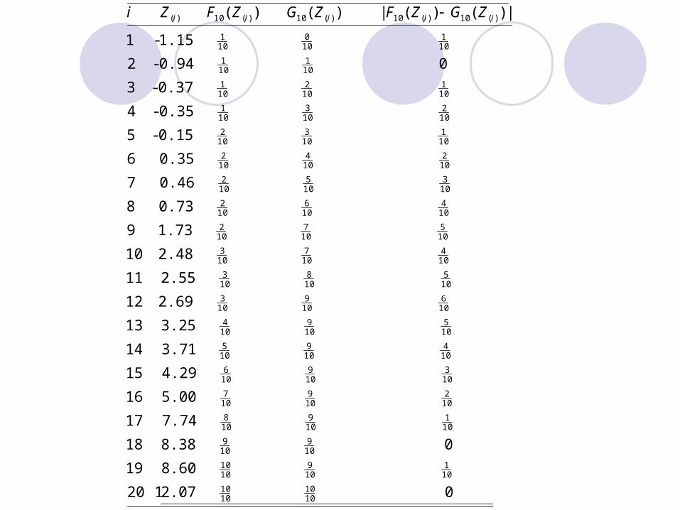
Since the sample sizes are both equal to 10, we arbitrarily choose to label the feedback group data as the X-sample and the no-feedback group data as the Y-sample. Thus we have m = n = 10, N = (10+10)=20,

and d = 10. We simultaneously illustrate the calculation of the values of the empirical distribution functions F10(t) and G10(t) at the ordered combined sample values Z(1) ≤…≤ Z(20) from Table 5.7, as well as the absolute differences | F10(Z(i) ) - G10(Z(i) )|, in the following display.

0 2.071 20

8.60 19

0 8.38 18

7.74 17

5.00 16

4.29 15

3.71 14

3.25 13

2.69 12

2.55 11

2.48 10

1.73 9

0.73 8

0.46 7

0.35 6

0.15- 5

0.35- 4

0.37- 3

0 0.94- 2

1.15- 1

|) ( ) (| ) ( ) (

1010

1010

101

109

1010

109

109

101

109

108

102

109

107

103

109

106

104

109

105

105

109

104

106

109

103

105

108

103

104

107

103

105

107

102

104

106

102

103

105

102

102

104

102

101

103

102

102

103

101

101

102

101

101

101

101

100

101

)(10)(10)(10)(10)( iiiii ZGZFZGZFZi

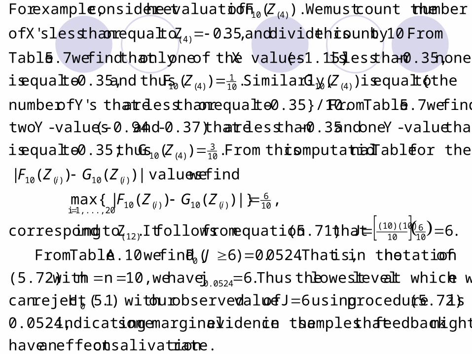
rate. salivationon effect an have

might feedback that samples in the evidence marginal some indicating 0.0524,

is (5.72) procedure using 6J of valueobservedour with )1.5( Hreject can

eat which w levellowest theThus .6j have we10,nm with (5.72)

ofnotation in the is,That .0524.0)6(P find weA.10 Table From

.6J that (5.71)equation from followsIt . Z toingcorrespond

,|}) ( ) (| {max

find we values|) ( ) (|

for the Table nalcomputatio thisFrom .)(G thus0.35;- toequal is

that value-Y one and 0.35- than less are that 0.37)- and (-0.94 values-Y two

find we5.7 Table From 0.35}/10.- toequalor than less are that sY' ofnumber

{the toequal is )(G Similarly, .)(F thusand 0.35,- toequal is

none 0.35,- than less is (-1.15) valuesX theof oneonly that find we5.7 Table

From 10.by count thisdivide and ,35.0 Z toequalor than less sX' of

number count themust We).(F of evaluation heconsider t example,For

0

0.0524

0

106

10(10)(10)

(12)

106

)(10)(101,...,20i

)(10)(10

103

)4(10

)4(10101

)4(10

(4)

)4(10

J

ZGZF

ZGZF

Z

ZZ

Z

ii

ii

atoccur can functionson distributi empirical Y and X in the jumps

themeshings, n

N theseofeach for Jfor n computatio in the now

that is tiesof case in the differenceonly The .

n

N1

prob has sY' and

sX' theof meshings possible n

N theofeach (5.1), Hunder that,

follows stillit 38,Comment in As s.X' as serving nsobservatio m and

sY' as serving nsobservation with nsobservatio N theof sassignment

possible allconsider toneed wes,Y'and/or sX' theamong ties

of presence in theeven level cesignificanexact test witha have To

with tiesJ ofon distributi lconditionaExact

0

n

N

:are J of valuesingcorrespond theand sassignment

ten These ns.observatio Y threeand nsobservatio X twoas serve to6.3

and 6.3, 3.2, 1.9, 1.9, nsobservatio theof sassignment possible 103

5

thegconsiderinby on distributi lconditiona itsobtain weJ, of value

thisof cesignifican theassess To .4| 0|6|)9.1( ).91 (|6

|) ( ) (|6|) ( ) (| is (5.71) J of value

ingcorrespond theand 3.6ZZ2.3Z9.1ZZ

:are values Zordered associated The

.3.6,9.1,9.1,3.6,2.3X :data 3n 2,m

following for theon constructi thisillustrate Wely.respective ,or

an greater th becan jumps theseof sizes theand nsobservatiocommon

32

32

)2(3)2(2)1(3)1(212(3)

(5)(4)(3)(2)(1)

(i)

32121

n1

m1

GF

ZGZFZGZF

YYYX

6 31.9,1.9,6. 3.6 ,.36

4 31.9,1.9,6. 3.6 ,.23

1 31.9,3.2,6. 3.6 ,9.1

1 31.9,3.2,6. 3.6 ,9.1

1 31.9,3.2,6. 3.6 ,9.1

1 31.9,3.2,6. 3.6 ,9.1

4 31.9,6.3,6. .23 ,9.1

4 31.9,6.3,6. 3.2 ,9.1

6 33.2,6.3,6. 9.1 ,9.1

J of Value Hunder y Probabilit nsObservatio nsObservatio

101

101

101

101

101

101

101

101

101

0YX

.1)1(P ,)4(P ,)6(P

iesprobabilit tailnull theyields This

0106

0102

0 JJJ

3 )1,1,,( (0,0,0,1)

2 )1,,,( (0,0,1,1)

2 )1,,,( (0,1,1,1)

3 )1,,(0, (1,1,1,1)

J )(G )(F Meshings

32

31

32

32

31

32

31

31

32

31

31

YYYX

YYXY

YXYY

XYYY

ZZ ii

:obtain weJ ofn computatio

for 5.4 Example ofapproach tabular theFollowing 5.d and 15,N

10,n 5,m have weHere .12,11,10,10

,8,7,6,4,4,3Y and 9,7

,5X ,3X ,3X :data tiedofset artificial following the

consider we ties,of case in the defined- wellis (5.71) expression

in given Jfor formula nalcomputatio thehow illustrate To

Ties

10987

65432154

321

YYYY

YYYYYXX

0 2.071 20

8.60 19

0 8.38 18

7.74 17

5.00 16

4.29 15

3.71 14

3.25 13

2.69 12

2.55 11

2.48 10

1.73 9

0.73 8

0.46 7

0.35 6

0.15- 5

0.35- 4

0.37- 3

0 0.94- 2

1.15- 1

|) ( ) (| ) ( ) (

1010

1010

101

109

1010

109

109

101

109

108

102

109

107

103

109

106

104

109

105

105

109

104

106

109

103

105

108

103

104

107

103

105

107

102

104

106

102

103

105

102

102

104

102

101

103

102

102

103

101

101

102

101

101

101

101

100

101

)(10)(10)(10)(10)( iiiii ZGZFZGZFZi

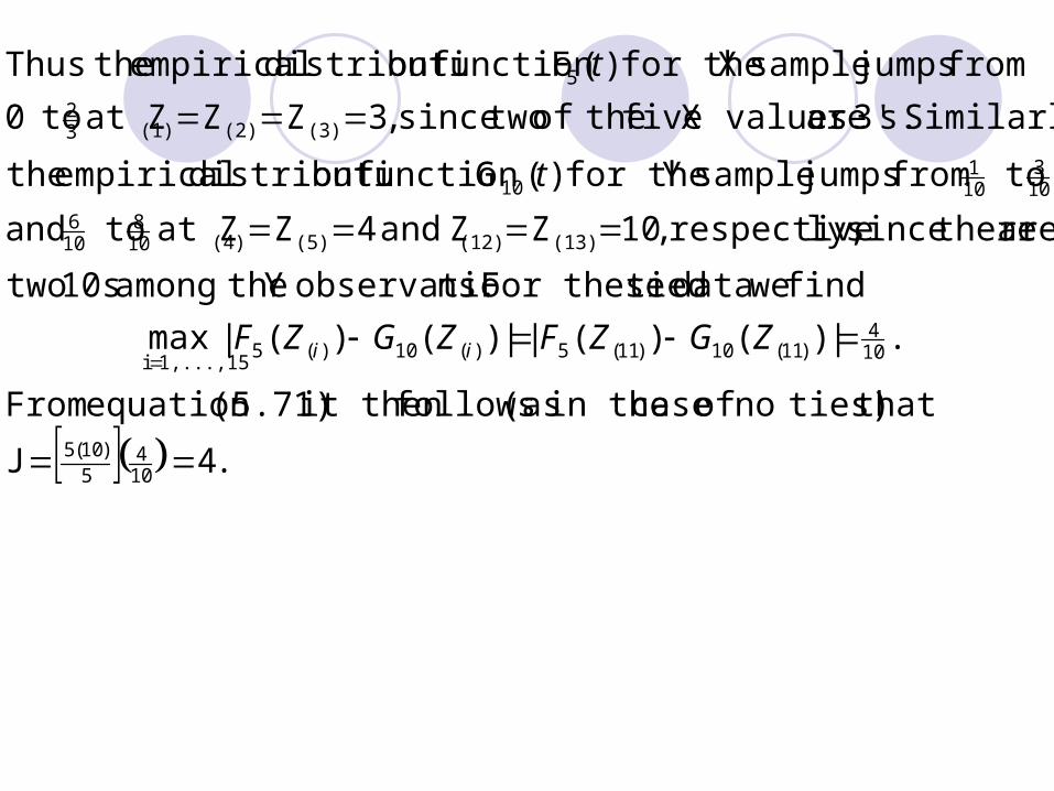
.4J

that ties)no of case in the (as followsit then (5.71)equation From

.|) ( ) (||) ( ) (|max

find wedata tiedFor these ns.observatio Y theamong 10s two

are theresince ly,respective ,10Z Zand 4Zat Z to and

to from jumps sample Y for the )(Gfunction on distributi empirical the

Similarly, s.3' are valuesX five theof twosince ,3ZZat Z to0

from jumps sample X for the )(Ffunction on distributi empirical theThus

104

5)10(5

104

)11(10)11(5)(10)(51,...,15i

(13)(12)(5)(4)108

106

103

101

10

(3)(2)(1)32

5

ZGZFZGZF

t

t

ii

c n,m, allfor )Pr()Pr(

)Pr()Pr(

:HUnder

}D,max{D D JClearly

)]()([maxD

)]()([maxD

|)()(|maxDLet

0

mnmndmn

mndmn

mn

mn

mn

cDcD

cDcD

GF

tGtF

tFtG

tFtG

nmmn

nmmn

nmt

mnt

mnt

(2n,0)}.at ng terminatibefore axis horizontal theabove unitsk

least at ofheight a with paths{}{Devent The n.mwhen

(2n,0)n)-mn,(mat end and (0,0)at start paths sample theAll

4.n 3,m XYYXXYY, Sample

:(1) of Proof

(2) 2

...3

2

2

222

)P(D

(1) 2

2

)P(D

m,nWhen

nn

nn

nn

nk

nk

nk

n

nkn

n

kn

n

kn

n

n

n

kn

n

.)DPr( ),0,(}{D As

1

2

1k-n

2nl)N(k,

2l, and 0between not isk If :1 Lemma

units.k ofheight a

reaching and (2n,2l) to(0,0) from paths ofnumber l)N(k,Let

2

2

nnnn

n

nkn

n

nk

nk kN

kn

n

anyway)k cross tohaspath

each ask reach tohas paths n that therestrictio he(without t

sY' lk-n and sX' lk-n have when wepaths of #

2l)-at(2n,2k end and (0,0)at start that paths of #l)N(k,

k. reaches

lastsit epoint wher theofright thepath to theofportion k that y

line about the reflectingby path ingcorrespond a is thereonce,least at k

level reaching and (2n,2l)at ending and (0,0)fron startingpath any For

Pra) QA278.8 Theory" ricNonparanet of Concepts" Gibbons &(Pratt

: 1 Lemma of Proof

}2Pr{D

}{DPr}{DPr}Pr{D So,

k.- andk both

reaching paths are thereas ,}{D}{D But,

}.{D}{D}{D

nn

nnnnnn

nnnn

nnnnnn

nk

nk

nk

nk

nk

nk

nk

nk

nk

l)k,N(j,-l)N(k,l)k,j,N(not

(3) symmetry by k,0)k,-2N(not

k,-k,0)N(not k,0)k,-N(not }{Din paths of no.

j.reach having

without k, reaching (2n,2l) to(0,0) from paths of no.l)k,j,N(not

first; j k, & j reaching (2n,2l) to(0,0) from paths of no.l)k,N(j,Let

nn

n

k

0.l)j,N(k, and l)-kk,N(j,l)-kN(j,

2l,-2kkjor 2l-2kkjWhen

l).j,N(k,-l)-kN(j,l)-kj,k,N(not

because is This

2l.-2kkjor

(4) 2l-2kkj if l)-kj,k,N(not

reflectionby l)-kk,N(j,l)k,N(j,

k,-2k)k,-N(not 2k-n

2n

k)N(k,-k,-k)N(-k,k)k,-k,N(not

k)k,-k,N(not k-n

2n

k,0)N(-k,-N(k,0)k,0)k,-N(not

(4),& 1 Lemma From

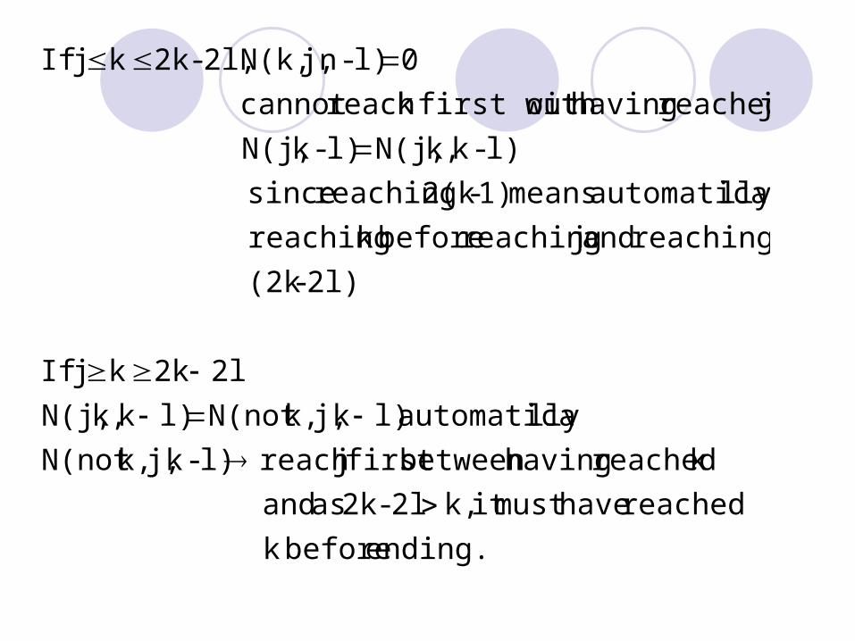
ending. beforek

reached havemust it k,2l-2k as and

k reached havingbetween first jreach l)-kj,k,N(not

llyautomatica l)kj,k,N(not l)kk,N(j,

2l2kkj If

2l)-(2k

reaching and j reaching beforek reaching

llyautomatica means 1)-2(k reaching since

l)-kk,N(j,l)-kN(j,

j reached havingout first withk reach cannot

0l)-nj,N(k, 2l,-2kkj If

(2). implieswhich

...3k-n

2n

2k-n

2n

k-n

2nk,0)k,-N(not

.k,-k,3k)..N(not 3k-n

2nk,-2k)k,-N(not

,Similarly

Large Sample Approximation

n

n

nkn

n

s

nn

nnnnn

nk

e

sDsD

))(1( )1)...(1)(-(1

...

.n as

]2n[sk

)Pr()Pr(

nk

nk

1nk

1-knk

knk

1knk1kn

knk-kn

1)1)...(n-kk)(n(n1)k-1)...(n-n(n

(2n)!k)!(nk)!(nn!n!2n!

2

2

2

n

2nk-n

2n

22

2

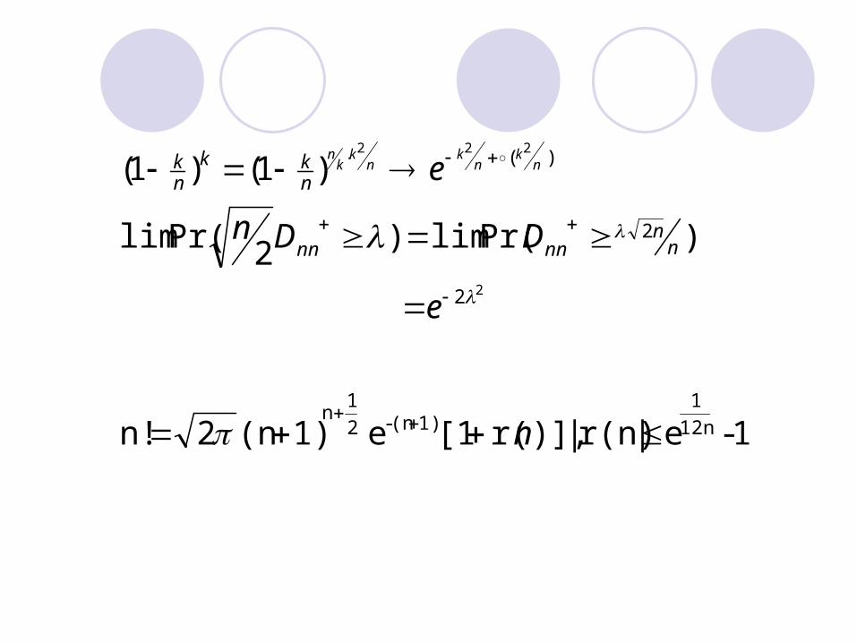
1-e|r(n)| )],r([1e 1)(n2n!

)Pr(lim)2Pr(lim

)1()1(

12n

11)(n-2

1n

2

2

)(

2

222

n

e

DDn

e

nn

nnnn

nkk

nk n

kn

kn

kk

n

e

1

e

1

)1()-(1

1

)1()-(1

1

)1()1()2(

)1()2(

)!()!(

)!(

2

1

)21(

11

)21(

1

2k)1()-k(1

11nk

2

1

12

1

1nk

)1()1(2

1

2

12

22122

2

2

2

nk

nk

kn

nk

kn

knknknkn

nn

n

nkn

n

nk

n

k

n

kkn

kn

n

knk

kn

e

eeknkn

en

knkn

n

22222

21

21

4s2s2s2s2s-

2222

21

12212

1111

)(

1

)(

1

* * *

)]1[()]1[(

])1[(])1[(

)1()1(*)1()1(

)1()1(

eeeee

sn

nssn

ns

n

nsn

ns

kn

kn

nn

nn

kn

n

kn

n

kkkk

kk

.)1(2

)Pr()Pr(

(2), From

]/[

1 n

2nik-n

2n

1

22

kn

i

i

nn

nnnnn sDsD

Hunder G F Note F. of free ison distributi limiting The

.)1()Pr(

)1(2)Pr(

,n as As

0.

22

1

212

2

n

2nik-n

2n

22

22

22

i

siinn

n

i

siinn

n

si

esD

esD

e

1

21

W& Hin J

nmmn

2nm

mn

mnmn

2

*

2

)1(2)Pr(

)Pr(

,n)min(m, as shown that becan It

n.m of case with thesame theare hence

and ,n & m howon dependnot do onsdistributi limitingtheir

that so edstandardizsuitably be tohave D & D n,mWhen

i

isimn

smn

esD

esD

jiij

jijijiG

k*kn

)t,(t

n1kn1n

jiij

jijijiF

k*km

)t,(t

k1km1m

k1

t tif)}F(t1){G(t

t tif)}G(t1){G(t)t,t( where

)(matrix covariance and

))t(G),...(G(tmean thehas ))t(G),...(t(G

t tif)}F(t1){F(t

t tif)}F(t1){F(t)t,(t

)(matrix , covariance and

))t(F),...t((Fmean a has ))t(F),...t((F

(distinct) t... tfixedarbitrary For

onillustrati heuristicA

jiG

jiF

covariance

2111

mean

kk11

0

)t,t()t,t(,)0,...,0,0(~

)(t)(t),...(t)(t

,:HUnder

mnmnnmmn FGFG

GF

§4.6 One Sample Goodness-of-Fit test

i

siin

n

nt

nt

nt

iid

n

esDn

tFtF

tFtF

tFtF

FFH

FXXX

2222/1

0

0n

0n

0n

00

0

21

)1()Pr(lim

,HUnder

|)()(|supD

|)()(|supD

|)()(|supD

Statistic Smirnov-Kolmogorov Sample One

:

.Fon distributi specified a from come data theif test Wish to

df) s(continuou ~,...,,

W.& Hin A.11 Table from found becan

.)1(2

)Pr(

where if Hreject tois

t oneleast at for )()(:H vsHfor test level An

,

1

21

,2/1

,2/1

0

010

2,

2

n

i

Dii

nn

nn

D

e

DDn

DDn

tFtF

n

Confidence Bands for F (unknown d.f.)

1) allfor )()()(Pr(lim

Then

]1,)(min[)(

]0,)(max[)(

n

2/,

2/,

xxUxFxL

xFxU

xFxL

nnn

n

D

nn

n

D

nn

n

n

statistic test Misesvon -reCram

)(])()([C

Ffor fit test -of-goodnessAnother

02

0n

xdFxFxFn n