Chapter 4. The Green Kubo Relations

4.1 The Langevin Equation

4.2 Mori-Zwanzig Theory

4.3 Shear Viscosity

4.4 Green-Kubo Relations for Navier-Stokes Transport

Coefficients

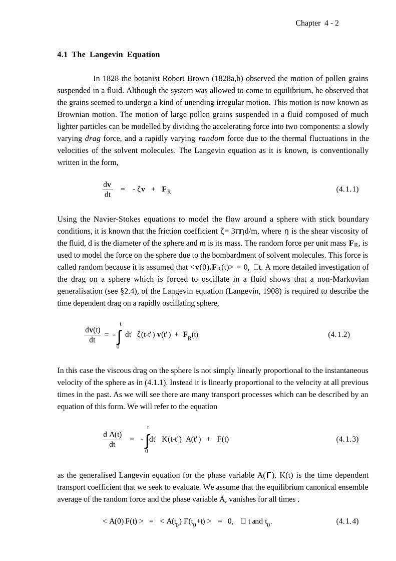
4.1 The Langevin Equation

In 1828 the botanist Robert Brown (1828a,b) observed the motion of pollen grains

suspended in a fluid. Although the system was allowed to come to equilibrium, he observed that

the grains seemed to undergo a kind of unending irregular motion. This motion is now known as

Brownian motion. The motion of large pollen grains suspended in a fluid composed of much

lighter particles can be modelled by dividing the accelerating force into two components: a slowly

varying drag force, and a rapidly varying random force due to the thermal fluctuations in the

velocities of the solvent molecules. The Langevin equation as it is known, is conventionally

written in the form,

dtdv

= - ζv + FR (4.1.1)

Using the Navier-Stokes equations to model the flow around a sphere with stick boundary

conditions, it is known that the friction coefficient ζ= 3πηd/m, where η is the shear viscosity of

the fluid, d is the diameter of the sphere and m is its mass. The random force per unit mass FR, is

used to model the force on the sphere due to the bombardment of solvent molecules. This force is

called random because it is assumed that <v(0).FR(t)> = 0, ∀ t. A more detailed investigation of

the drag on a sphere which is forced to oscillate in a fluid shows that a non-Markovian

generalisation (see §2.4), of the Langevin equation (Langevin, 1908) is required to describe the

time dependent drag on a rapidly oscillating sphere,

dt

dv(t) = - ∫

0

t

dt' ζ(t-t' ) v(t' ) + FR(t) (4.1.2)

In this case the viscous drag on the sphere is not simply linearly proportional to the instantaneous

velocity of the sphere as in (4.1.1). Instead it is linearly proportional to the velocity at all previous

times in the past. As we will see there are many transport processes which can be described by an

equation of this form. We will refer to the equation

dt

d A(t) = - ∫

0

t

dt' K(t-t' ) A(t' ) + F(t) (4.1.3)

as the generalised Langevin equation for the phase variable A(ΓΓΓΓ ). K(t) is the time dependent

transport coefficient that we seek to evaluate. We assume that the equilibrium canonical ensemble

average of the random force and the phase variable A, vanishes for all times .

< A(0) F(t) > = < A(t0) F(t0+t) > = 0, ∀ t and t0. (4.1.4)

Chapter 4 - 2

The time displacement by t0 is allowed because the equilibrium time correlation function is

independent of the time origin. Multiplying both sides of (4.1.3) by the complex conjugate of A(0)

and taking a canonical average we see that,

dt

d C(t) = - ∫

0

t

dt' K(t-t' ) C(t' ) (4.1.5)

where C(t) is defined to be the equilibrium autocorrelation function,

C(t) ≡ < A(t) A* (0) >. (4.1.6)

Another function we will find useful is the flux autocorrelation function φ(t)

φ(t) = < .A(t)

.A* (0) >. (4.1.7)

Taking a Laplace transform of (4.1.5) we see that there is a intimate relationship between the

transport memory kernel K(t) and the equilibrium fluctuations in A. The left-hand side of (4.1.5)

becomes

∫0

∞

dt e-st dt

dC(t) = e

-st C(t) 0

∞ - ∫

0

∞

dt (-se-st) C(t) = s∼C(s) - C(0),

and as the right-hand side is a Laplace transform convolution,

sC~(s) - C(0) = - K

~(s) C

~(s) (4.1.8)

So that

C~(s) =

s + K~(s)

C(0)(4.1.9)

One can convert the A autocorrelation function into a flux autocorrelation function by realising that,

dt2

d2 C(t)

= dtd <

dtdA(t)

A* (0) > = dtd < [iLA(t)] A * (0) >

= dtd < A(t) [-iLA * (0)] > = - < [iLA(t)] [-iLA *(0)] > = - φ(t).

Chapter 4 - 3

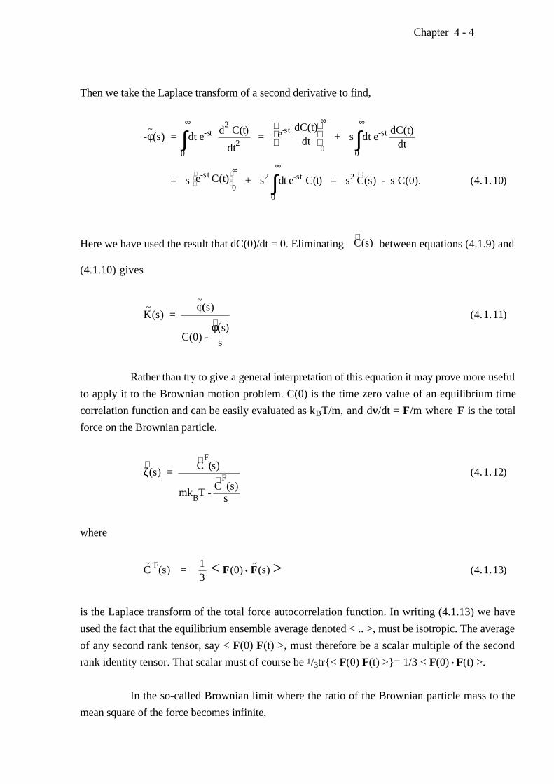
Then we take the Laplace transform of a second derivative to find,

-φ~(s) = ∫

0

∞

dt e-st dt2

d2 C(t)

= e-st

dtdC(t)

0

∞

+ s ∫0

∞

dt e-st dt

dC(t)

= s e-st C(t)

0

∞ + s2 ∫

0

∞

dt e-st C(t) = s2 ∼C(s) - s C(0). (4.1.10)

Here we have used the result that dC(0)/dt = 0. Eliminating ∼C(s) between equations (4.1.9) and

(4.1.10) gives

K~(s) =

C(0) - sφ∼ (s)

φ~(s)

(4.1.11)

Rather than try to give a general interpretation of this equation it may prove more useful

to apply it to the Brownian motion problem. C(0) is the time zero value of an equilibrium time

correlation function and can be easily evaluated as kBT/m, and dv/dt = F/m where F is the total

force on the Brownian particle.

∼ζ(s) =

mkBT - s

∼C

F(s)

∼C

F(s)

(4.1.12)

where

C~ F(s) =

31

< F(0) • F~(s) > (4.1.13)

is the Laplace transform of the total force autocorrelation function. In writing (4.1.13) we have

used the fact that the equilibrium ensemble average denoted < .. >, must be isotropic. The average

of any second rank tensor, say < F(0) F(t) >, must therefore be a scalar multiple of the second

rank identity tensor. That scalar must of course be 1/3tr< F(0) F(t) >= 1/3 < F(0) • F(t) >.

In the so-called Brownian limit where the ratio of the Brownian particle mass to the

mean square of the force becomes infinite,

Chapter 4 - 4

∼ζ(s) = 3mβ

∫0

∞

dt e-st < F(t) • F(0) > (4.1.14)

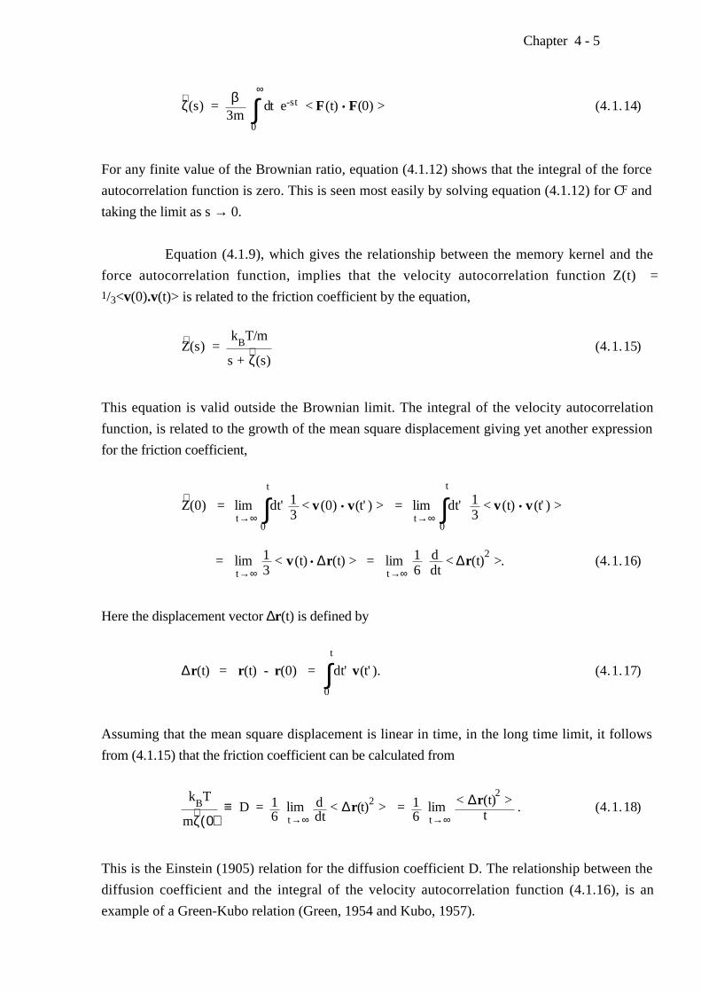
For any finite value of the Brownian ratio, equation (4.1.12) shows that the integral of the force

autocorrelation function is zero. This is seen most easily by solving equation (4.1.12) for CF and

taking the limit as s → 0.

Equation (4.1.9), which gives the relationship between the memory kernel and the

force autocorrelation function, implies that the velocity autocorrelation function Z(t) = 1/3<v(0).v(t)> is related to the friction coefficient by the equation,

∼Z(s) = s +

∼ζ(s)

kBT/m

(4.1.15)

This equation is valid outside the Brownian limit. The integral of the velocity autocorrelation

function, is related to the growth of the mean square displacement giving yet another expression

for the friction coefficient,

∼Z(0) = lim

t→∞ ∫

0

t

dt' 31 < v(0) • v(t' ) > = lim

t→∞ ∫

0

t

dt' 31 < v(t) • v(t' ) >

= limt→∞

31 < v(t) • ∆r(t) > = lim

t→∞ 6

1 dtd < ∆r(t)

2 >. (4.1.16)

Here the displacement vector ∆r (t) is defined by

∆r(t) = r(t) - r(0) = ∫0

t

dt' v(t' ). (4.1.17)

Assuming that the mean square displacement is linear in time, in the long time limit, it follows

from (4.1.15) that the friction coefficient can be calculated from

m

∼ζ(0)

kBT

≡ D = 61 lim

t→∞

dtd < ∆r(t)2 > =

61 lim

t→∞ t

< ∆r(t)2 > . (4.1.18)

This is the Einstein (1905) relation for the diffusion coefficient D. The relationship between the

diffusion coefficient and the integral of the velocity autocorrelation function (4.1.16), is an

example of a Green-Kubo relation (Green, 1954 and Kubo, 1957).

Chapter 4 - 5

It should be pointed out that the transport properties we have just evaluated are

properties of systems at equilibrium. The Langevin equation describes the irregular Brownian

motion of particles in an equilibrium system. Similarly the self diffusion coefficient characterises

the random walk executed by a particle in an equilibrium system. The identification of the zero

frequency friction coefficient 6πηd/m, with the viscous drag on a sphere which is forced to move

with constant velocity through a fluid, implies that equilibrium fluctuations can be modelled by

nonequilibrium transport coefficients, in this case the shear viscosity of the fluid. This hypothesis

is known as the Onsager regression hypothesis (Onsager, 1931). The hypothesis can be inverted:

one can calculate transport coefficients from a knowledge of the equilibrium fluctuations. We will

now discuss these relations in more detail.

Chapter 4 - 6

4.2 Mori-Zwanzig Theory

We will show that for an arbitrary phase variable A(ΓΓΓΓ ), evolving under equations of

motion which preserve the equilibrium distribution function, one can always write down a

Langevin equation. Such an equation is an exact consequence of the equations of motion. We will

use the symbol iL, to denote the Liouvillean associated with these equations of motion. These

equilibrium equations of motion could be field-free Newtonian equations of motion or they could

be field-free thermostatted equations of motion such as Gaussian isokinetic or Nosé-Hoover

equations. The equilibrium distribution could be microcanonical, canonical or even isothermal-

isobaric provided that if the latter is the case, suitable distribution preserving dynamics are

employed. For simplicity we will compute equilibrium time correlation functions over the

canonical distribution function, fc,

fc(ΓΓΓΓ ) =

∫ dΓΓΓΓ e-βH0(ΓΓΓΓ )

e-βH0(ΓΓΓΓ )

(4.2.1)

We saw in the previous section that a key element of the derivation was that the correlation of the

random force, FR(t) with the Langevin variable A, vanished for all time. We will now use the

notation first developed in §3.5, which treats phase variables, A(ΓΓΓΓ ), B(ΓΓΓΓ ), as vectors in 6N-

dimensional phase space with a scalar product defined by ∫dΓΓΓΓ f 0 (ΓΓΓΓ)B(ΓΓΓΓ)A*(ΓΓΓΓ), and denoted as

(B,A*). We will define a projection operator which will transform any phase variable B, into a

vector which has no correlation with the Langevin variable, A. The component of B parallel to A is

just,

P B(ΓΓΓΓ ,t) = (A(ΓΓΓΓ ),A*(ΓΓΓΓ ))

(B(ΓΓΓΓ , t),A*(ΓΓΓΓ )) A(ΓΓΓΓ ). (4.2.2)

This equation defines the projection operator P.

The operator Q=1-P, is the complement of P and computes the component of B

orthogonal to A.

(QB(t),A* ) = (B(t) - (A,A* )

(B(t),A*) A, A* )

= (B(t),A*) - (A,A* )

(B(t),A* ) (A,A* ) = 0 (4.2.3)

In more physical terms the projection operator Q computes that part of any phase variable which is

random with respect to a Langevin variable, A.

Chapter 4 - 7

A*

B

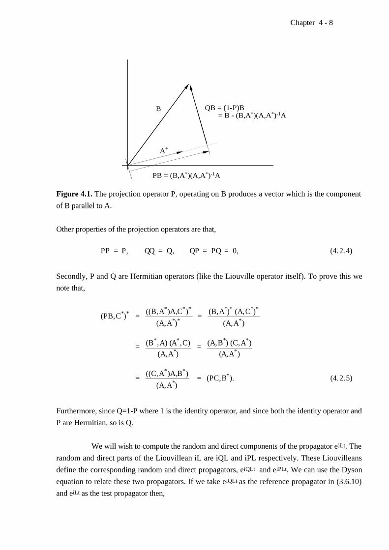
PB = (B,A*)(A,A*)-1A

QB = (1-P)B = B - (B,A*)(A,A*)-1A

Figure 4.1. The projection operator P, operating on B produces a vector which is the component

of B parallel to A.

Other properties of the projection operators are that,

PP = P, QQ = Q, QP = PQ = 0, (4.2.4)

Secondly, P and Q are Hermitian operators (like the Liouville operator itself). To prove this we

note that,

(PB,C*)* = (A,A*)*

((B,A* )A,C* )* =

(A,A* )

(B,A*)* (A,C*)*

= (A,A*)

(B* ,A) (A* ,C) = (A,A* )

(A,B*) (C,A*)

= (A,A*)

((C,A* )A,B* ) = (PC,B* ). (4.2.5)

Furthermore, since Q=1-P where 1 is the identity operator, and since both the identity operator and

P are Hermitian, so is Q.

We will wish to compute the random and direct components of the propagator eiLt . The

random and direct parts of the Liouvillean iL are iQL and iPL respectively. These Liouvilleans

define the corresponding random and direct propagators, eiQLt and eiPLt. We can use the Dyson

equation to relate these two propagators. If we take eiQLt as the reference propagator in (3.6.10)

and eiLt as the test propagator then,

Chapter 4 - 8

eiLt = eiQLt + ∫0

t

dτ eiL(t- τ) iPL eiQLτ. (4.2.6)

The rate of change of A(t), the Langevin variable at time t is,

dt

d A(t) = eiLt iLA = eiLt i(Q + P) LA. (4.2.7)

But,

eiLt iPLA = eiLt (A,A* )

(iLA,A * ) A = (A,A* )

(iLA,A * ) eiLt A ≡ iΩ A(t). (4.2.8)

This defines the frequency iΩ which is an equilibrium property of the system. It only involves

equal time averages. Substituting this equation into (4.2.7) gives,

dt

dA(t) = iΩ A(t) + eiLt iQLA. (4.2.9)

Using the Dyson decomposition of the propagator given in equation (4.2.6), this leads to,

dt

dA(t) = iΩ A(t) + ∫0

t

dτ eiL(t- τ) iPL eiQLτ iQLA + eiQLt iQLA. (4.2.10)

We identify eiQLt iQLA as the random force F(t) because,

(F(t),A*) = (eiQLt iQLA,A* ) = (QF(t),A* ) = 0, (4.2.11)

where we have used (4.2.4). It is very important to remember that the propagator which generates

F(t) from F(0) is not the propagator eiLt , rather it is the random propagator eiQLt. The integral in

(4.2.10) involves the term,

iPL eiQLt

iQLA = iPLF(t) = iPLQF(t)

= (A,A* )

(iLQF(t),A* ) A

= - (A,A* )

(QF(t),(iLA)* ) A

as L is Hermitian and i is anti-Hermitian, (iL)*=(d/dt)*=(dΓΓΓΓ /dt•d/dΓΓΓΓ )∗ =d/dt=iL, (since the

Chapter 4 - 9

equations of motion are real). Since Q is Hermitian,

iPL eiQLt

iQLA = - (A,A* )

(F(t),(QiLA)*) A

= - (A,A* )

(F(t),F(0)* ) A ≡ - K(t) A, (4.2.12)

where we have defined a memory kernel K(t). It is basically the autocorrelation function of the

random force. Substituting this definition into (4.2.10) gives

dt

dA(t) = iΩ A(t) - ∫

0

t

dτ eiL(t-τ)

K(τ) A + F(t)

= iΩ A(t) - ∫0

t

dτ K(τ) A(t-τ) + F(t). (4.2.13)

This shows that the Generalised Langevin Equation is an exact consequence of the equations of

motion for the system (Mori, 1965a, b; Zwanzig, 1961). Since the random force is random with

respect to A, multiplying both sides of (4.2.13) by A*(0) and taking a canonical average gives the

memory function equation,

dt

dC(t) = iΩ C(t) - ∫0

t

dτ K(τ) C(t-τ). (4.2.14)

This is essentially the same as equation (4.1.5).

As we mentioned in the introduction to this section the generalised Langevin equation

and the memory function equation are exact consequences of any dynamics which preserves the

equilibrium distribution function. As such the equations therefore describe equilibrium fluctuations

in the phase variable A, and the equilibrium autocorrelation function for A, namely C(t).

However the generalised Langevin equation bears a striking resemblance to a

nonequilibrium constitutive relation. The memory kernel K(t) plays the role of a transport

coefficient. Onsager's regression hypothesis (1931) states that the equilibrium fluctuations in a

phase variable are governed by the same transport coefficients as is the relaxation of that same

phase variable to equilibrium. This hypothesis implies that the generalised Langevin equation can

be interpreted as a linear, nonequilibrium constitutive relation with the memory function K(t),

given by the equilibrium autocorrelation function of the random force.

Chapter 4 - 10

Onsager's hypothesis can be justified by the fact that in observing an equilibrium

system for a time which is of the order of the relaxation time for the memory kernel, it is

impossible to tell whether the system is at equilibrium or not. We could be observing the final

stages of a relaxation towards equilibrium or, we could be simply observing the small time

dependent fluctuations in an equilibrium system. On a short time scale there is simply no way of

telling the difference between these two possibilities. When we interpret the generalised Langevin

equation as a nonequilibrium constitutive relation, it is clear that it can only be expected to be valid

close to equilibrium. This is because it is a linear constitutive equation.

Chapter 4 - 11

4.3 Shear Viscosity

It is relatively straightforward to apply the Mori-Zwanzig formalism to the calculation

of fluctuation expressions for linear transport coefficients. Our first application of the method will

be the calculation of shear viscosity. Before we do this we will say a little more about about

constitutive relations for shear viscosity. The Mori-Zwanzig formalism leads naturally to a non-

Markovian expression for the viscosity. Equation (4.2.13) refers to a memory function rather than

a simple Markovian transport coefficient such as the Newtonian shear viscosity. We will thus be

lead to a discussion of viscoelasticity (see §2.4).

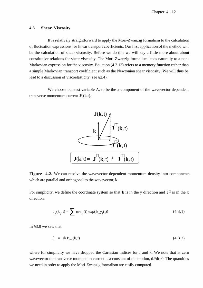
We choose our test variable A, to be the x-component of the wavevector dependent

transverse momentum current J⊥ (k,t).

k

J(k, t)

J

(k, t)

J(k, t)= J⊥(k, t) + J

(k, t)

J⊥(k, t)

Figure 4.2. We can resolve the wavevector dependent momentum density into components

which are parallel and orthogonal to the wavevector, k.

For simplicity, we define the coordinate system so that k is in the y direction and J⊥ is in the x

direction.

Jx(k

y,t) = ∑ mv

xi(t) exp(ik

yy

i(t)) (4.3.1)

In §3.8 we saw that

.J = ik Pyx(k,t) (4.3.2)

where for simplicity we have dropped the Cartesian indices for J and k. We note that at zero

wavevector the transverse momentum current is a constant of the motion, dJ/dt=0. The quantities

we need in order to apply the Mori-Zwanzig formalism are easily computed.

Chapter 4 - 12

The frequency matrix iΩ, defined in (4.2.8), is identically zero. This is always so in the

single variable case as -<A*dA/dt> = 0, for any phase variable A. The norm of the transverse

current is calculated

(J(k),J*(k)) = < ∑

i=1

N

pxi

eiky i

∑j =1

N

pxj

e-iky j

>

= N<px12 > + N(N-1) <p

x1p

x2 e

ik(y1-y2) >

= NmkBT (4.3.3)

At equilibrium pxi is independent of px2 and (y1-y2) so the correlation function factors into the

product of three equilibrium averages. The values of <px1> and <px2> are identically zero. The

random force, F, can also easily be calculated since

P Pyx(k) = < | J(k) |

2>

(Pyx(k),J(-k)) J = 0, (4.3.4)

we can write,

F(0) = iQLJ = (1-P) ik Pyx(k) = ik Pyx(k). (4.3.5)

The time dependent random force (see (4.2.11)), is

F(t) = eiQLt ik Pyx

(k) (4.3.6)

A Dyson decomposition of eQiLt in terms of eiLt shows that,

eiLt = eQiLt + ∫0

t

ds eiL(t-s) PiL eQiLs (4.3.7)

Now for any phase variable B,

PiLB = < J*iLB >

NmkBT

J = -< B(iLJ)

*>

NmkBT

J

= - ik<BPyx

(-k)>Nmk

BT (4.3.8)

J

Chapter 4 - 13

Substituting this observation into (4.3.7) shows that the difference between the propagators eQiLt

and eiLt is of order k, and can therefore be ignored in the zero wavevector limit.

From equation (4.2.12) the memory kernel K(t) is <F(t)F* (0)>/ <AA * >. Using

equation (4.3.6), the small wavevector form for K(t) becomes,

K(t) = k2 Nmk

BT

< Pyx

(k,t) Pyx

(-k,0)>(4.3.9)

The generalised Langevin equation (the analogue of equation 4.2.13) is

lim dt

dJx(k

y, t)

= NmkBT

-k2

∫0

t

ds < Pyx

(ky,s) P

yx(-k

y,0) >

0 J

x(k

y, t-s)

k→0

+ iky P

yx(k

y,t) (4.3.10)

where we have taken explicit note of the Cartesian components of the relevant functions. Now we

know that the rate of change of the transverse current is ik Pyx(k,t). This means that the left hand

side of (4.3.10) is related to equilibrium fluctuations in the shear stress. We also know that J(k)

=∫ dk' ρ(k'-k) u(k'), so, close to equilibrium, the transverse momentum current (our Langevin

variable A), is closely related to the wavevector dependent strain rate γ(k). In fact the wavevector

dependent strain rate γ(k) is -ikJ(k)/ρ(k=0). Putting these two observations together we see that

the generalised Langevin equation for the transverse momentum current is essentially a relation

between fluctuations in the shear stress and the strain rate - a constitutive relation. Ignoring the

random force (constitutive relations are deterministic), we find that equation (4.3.10) can be

written in the form of the constitutive relation (2.4.12),

lim Pyx

(t) = - ∫0

t

ds η(k=0,t-s) γ(k=0,s)k→0

(4.3.11)

If we use the fact that, PyxV = lim(k→0) Pyx(k), η(t) is easily seen to be

η(t) = βV < Pxy

(t) Pxy

(0) > (4.3.12)

Equation (4.3.11) is identical to the viscoelastic generalisation of Newton's law of viscosity

equation (2.4.12).

The Mori-Zwanzig procedure has derived a viscoelastic constitutive relation. No

mention has been made of the shearing boundary conditions required for shear flow. Neither is

Chapter 4 - 14

there any mention of viscous heating or possible nonlinearities in the viscosity coefficient.

Equation (4.3.10) is a description of equilibrium fluctuations. However unlike the case for the

Brownian friction coefficient or the self diffusion coefficient, the viscosity coefficient refers to

nonequilibrium rather than equilibrium systems.

The zero wavevector limit is subtle. We can imagine longer and longer wavelength

fluctuations in the strain rate γ(k). For an equilibrium system however γ(k=0) ≡ 0 and < γ(k=0)

γ∗ (k=0) > ≡ 0. There are no equilibrium fluctuations in the strain rate at k=0. The zero

wavevector strain rate is completely specified by the boundary conditions.

If we invoke Onsager's regression hypothesis we can obviously identify the memory

kernel η(t) as the memory function for planar (ie. k=0) Couette flow. We might observe that there

is no fundamental way of knowing whether we are watching small equilibrium fluctuations at

small but non-zero wavevector, or the last stages of relaxation toward equilibrium of a finite k,

nonequilibrium disturbance. Provided the nonequilibrium system is sufficiently close to

equilibrium, the Langevin memory function will be the nonequilibrium memory kernel. However

the Onsager regression hypothesis is additional to, and not part of, the Mori-Zwanzig theory. In

§6.3 we prove that the nonequilibrium linear viscosity coefficient is given exactly by the infinite

time integral of the stress fluctuations. In §6.3 we will not use the Onsager regression hypothesis.

At this stage one might legitimately ask the question: what happens to these equations if

we do not take the zero wavevector limit? After all we have already defined a wavevector

dependent shear viscosity in (2.4.13). It is not a simple matter to apply the Mori-Zwanzig

formalism to the finite wavevector case. We will instead use a method which makes a direct appeal

to the Onsager regression hypothesis.

Provided the time and spatially dependent strain rate is of sufficiently small amplitude,

the generalised viscosity can be defined as (2.4.13),

Pyx

(k,t) = - ∫0

t

ds η(k, t-s) γ(k,s) (4.3.13)

Using the fact that γ(k,t) = -ikux(k,t) = -ikJ(k,t)/ρ, and that dJ(k,t)/dt = ikPyx(k,t), we can rewrite

(4.3.13) as,

J(k,t) = - ρk

2

∫0

t

ds η(k, t-s) J(k,s)•

(4.3.14)

If we Fourier-Laplace transform both sides of this equation in time, and using Onsager's

Chapter 4 - 15

hypothesis, multiply both sides by J(-k,0) and average with respect to the equilibrium canonical

ensemble we obtain,

C~(k,ω) =

iω + ρ

k2η~(k,ω)

C(k,0)(4.3.15)

where C(k,t) is the equilibrium transverse current autocorrelation function <J(k,t) J(-k,0)> and the

tilde notation denotes a Fourier-Laplace transform in time,

∼C(ω) = ∫0

∞

dt C(t) e-iωt . (4.3.16)

We call the autocorrelation function of the wavevector dependent shear stress,

N(k,t) ≡ Vk

BT

1 < P

yx(k,t) P

yx(-k,0) > (4.3.17)

We can use the relation dJ(k,t)/dt = ikPyx(k,t), to transform from the transverse current

autocorrelation function C(k,t) to the stress autocorrelation function N(k,t) since,

dt2d

2 < J(k,t) J(-k,0) > = - <

.J(k,t)

.J(-k,0) >

= - k2 < Pyx(k,t) Pyx(-k,0) > (4.3.18)

This derivation closely parallels that for equation (4.1.10) and (4.1.11) in §4.1. The reader should

refer to that section for more details. Using the fact that, ρ=Nm/V, we see that,

k2 VkBT N~(k,ω) = ω2 C~(k,ω) + iω C(k,0). (4.3.19)

The equilibrium average C(k,0) is given by equation (4.3.3). Substituting this equation into

equation (4.3.15) gives us an equation for the frequency and wavevector dependent shear viscosity

in terms of the stress autocorrelation function,

η~(k,ω) =

1 - iωρ

k2 N~

(k,ω)

N~(k,ω)

(4.3.20)

Chapter 4 - 16

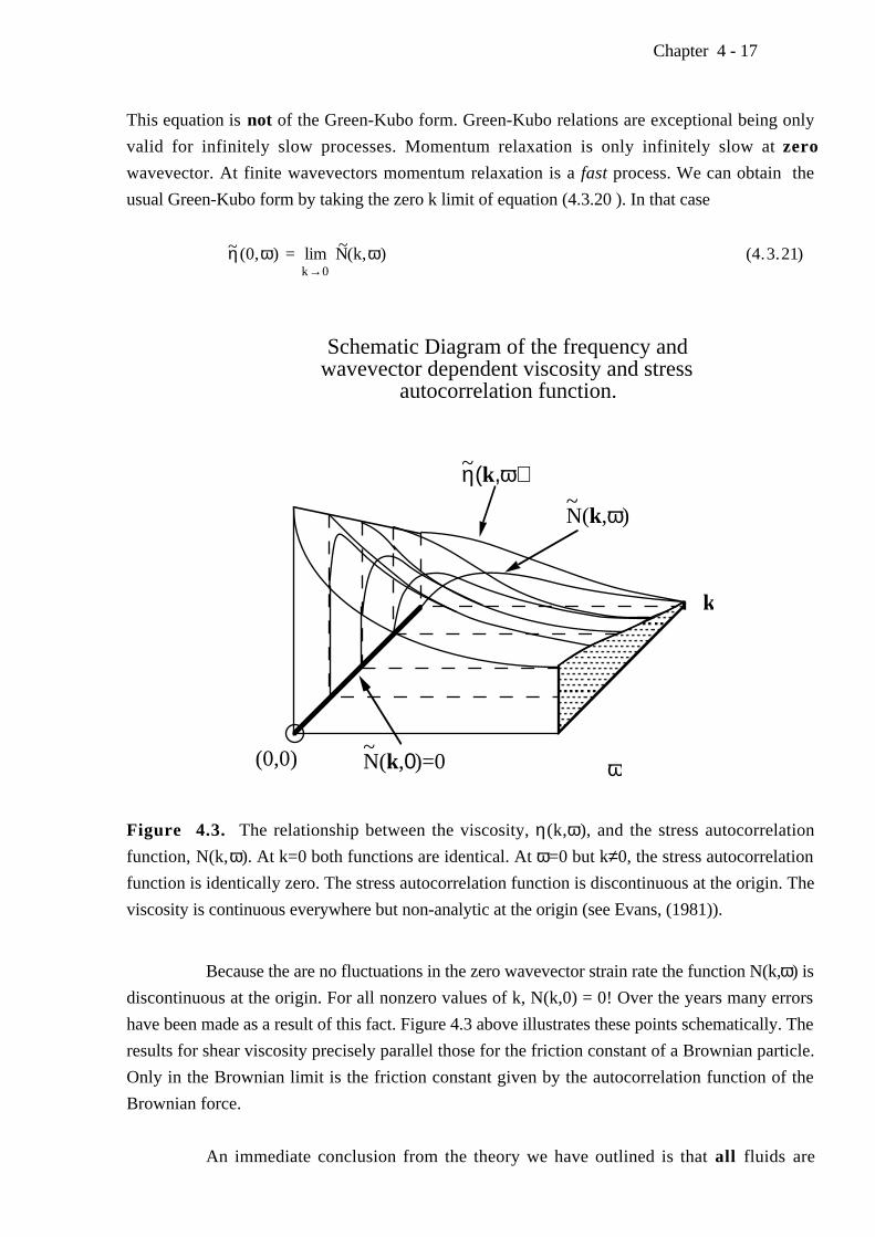
This equation is not of the Green-Kubo form. Green-Kubo relations are exceptional being only

valid for infinitely slow processes. Momentum relaxation is only infinitely slow at zero

wavevector. At finite wavevectors momentum relaxation is a fast process. We can obtain the

usual Green-Kubo form by taking the zero k limit of equation (4.3.20 ). In that case

η~(0,ω) = lim N~(k,ω)k→0

(4.3.21)

k

ω

η(k,ω)~

N(k,ω)~

Schematic Diagram of the frequency and wavevector dependent viscosity and stress

autocorrelation function.

(0,0) N(k,0)=0~

Figure 4.3. The relationship between the viscosity, η(k,ω), and the stress autocorrelation

function, N(k,ω). At k=0 both functions are identical. At ω=0 but k≠0, the stress autocorrelation

function is identically zero. The stress autocorrelation function is discontinuous at the origin. The

viscosity is continuous everywhere but non-analytic at the origin (see Evans, (1981)).

Because the are no fluctuations in the zero wavevector strain rate the function N(k,ω) is

discontinuous at the origin. For all nonzero values of k, N(k,0) = 0! Over the years many errors

have been made as a result of this fact. Figure 4.3 above illustrates these points schematically. The

results for shear viscosity precisely parallel those for the friction constant of a Brownian particle.

Only in the Brownian limit is the friction constant given by the autocorrelation function of the

Brownian force.

An immediate conclusion from the theory we have outlined is that all fluids are

Chapter 4 - 17

viscoelastic. Viscoelasticity is a direct result of the Generalised Langevin equation which is in turn

an exact consequence of the microscopic equations of motion.

Chapter 4 - 18

4 . 4 Green-Kubo Relations for Navier-Stokes Transport Coefficients

It is relatively straightforward to derive Green-Kubo relations for the other Navier-

Stokes transport coefficients, namely bulk viscosity and thermal conductivity. In §6.3 when we

describe the SLLOD equations of motion for viscous flow we will find a simpler way of deriving

Green-Kubo relations for both viscosity coefficients. For now we simply state the Green-Kubo

relation for bulk viscosity as (Zwanzig, 1965),

η = Vk

BT

1 ∫

0

∞

dt < [ p(t)V(t) - <pV> ][ p(0)V(0) - <pV> ] >V

(4.4.1)

The Green-Kubo relation for thermal conductivity can be derived by similar arguments

to those used in the viscosity derivation. Firstly we note from (2.1.26), that in the absence of a

velocity gradient, the internal energy per unit volume ρU obeys a continuity equation, ρdU/dt = -

∇∇∇∇ •JQ. Secondly, we note that Fourier's definition of the thermal conductivity coefficient λ, from

equation (2.3.16a), is JQ = -λ ∇∇∇∇ T. Combining these two results we obtain

ρ dtdU = λ ∇ 2T . (4.4.2)

Unlike the previous examples, both U and T have nonzero equilibrium values; namely, <U> and

<T>. A small change in the left-hand side of equation (4.4.2) can be written as (ρ+∆ρ)

d(<U>+∆U)/dt. By definition d<U>/dt=0, so to first order in ∆, we have ρd∆U/dt. Similarly, the

spatial gradient of <T> does not contribute, so we can write

ρ dt

d∆U = λ ∇ 2 ∆T . (4.4.3)

The next step is to relate the variation in temperature ∆T to the variation in energy per

unit volume ∆(ρU). To do this we use the thermodynamic definition,

V1

∂T∂E |

V =

∂T∂(ρU)

|V

= ρcV (4.4.4)

where cV is the specific heat per unit mass. We see from the second equality, that a small variation

in the temperature ∆T is equal to ∆(ρU)/ρcV. Therefore,

ρ.

∆U = ρcV

λ ∇ 2ρ∆U (4.4.5)

Chapter 4 - 19

If DT ≡ λ/ρcV is the thermal diffusivity, then in terms of the wavevector dependent internal energy

density equation (4.4.5) becomes,

ρ∆.U(k ,t) = - k2D

T ρ∆U(k, t) (4.4.6)

If C(k,t) is the wavevector dependent internal energy density autocorrelation function,

C(k,t) ≡ < ρ∆U(k , t) ρ∆U(-k ,0) > (4.4.7)

then the frequency and wavevector dependent diffusivity is the memory function of energy density

autocorrelation function,

∼C(k,ω) =

iω + k2 ∼D

T(k,ω)

C(k,0)(4.4.8)

Using exactly the same procedures as in §4.1 we can convert (4.4.8) to an expression for the

diffusivity in terms of a current correlation function. From (4.1.7 & 10) if φ = - d2C/dt2 then,

φ(k,t) = k2< JQx

(k,t) JQx

(-k,0) > (4.4.9)

Using equation (4.1.10), we obtain the analogue of (4.1.11),

k2 ∼DT(k,ω) = ∼C(k,ω)

C(k,0) - iω∼C(k,ω)

=

C(k,0) - iω

∼φ(k,ω)

∼φ(k,ω) . (4.4.10)

If we define the analogue of equation (4.3.17), that is φ(k,t) = k2 NQ(k,t), then equation (4.4.10)

for the thermal diffusivity can be written in the same form as the wavevector dependent shear

viscosity equation (4.3.20). That is

∼DT(k,ω) =

C(k,0) - iωk

2

∼N

Q(k,ω)

∼N

Q(k,ω)

. (4.4.11)

Again we see that we must take the zero wavevector limit before we take the zero frequency limit,

and using the canonical ensemble fluctuation formula for the specific heat,

ρcCVk TV

B

= ( , )0 02 (4.4.12)

Chapter 4 - 20

we obtain the Green-Kubo expression for the thermal conductivity

λ = k

BT

2

V ∫

0

∞

dt < JQx

(t) JQx

(0) > . (4.4.13)

This completes the derivation of Green-Kubo formula for thermal transport coefficients. These

formulae relate thermal transport coefficients to equilibrium properties. In the next chapter we will

develop nonequilibrium routes to the thermal transport coefficients.

Chapter 4 - 21