1

Chapter 4 (Part 2):Artificial Neural Networks

CS 536: Machine LearningLittman (Wu, TA)

AdministrationiCML-03: instructional Conference on

Machine Learninghttp://www.cs.rutgers.edu/~mlittman/courses/ml03/iCML03/Weka exercisehttp://www.cs.rutgers.edu/~mlittman/courses/ml03/hw1.pdf

2

Grading Components• HWs (not handed in): 0%• Project paper (iCML): 25%

– document (15%), review (5%),revision(5%)

• Project presentation: 20%– oral (10%), slides (10%)

• Midterm (take home): 20%• Final: 35%

Artificial Neural Networks[Read Ch. 4]

[Review exercises 4.1, 4.2, 4.5, 4.9, 4.11]• Threshold units [ok]• Gradient descent [today]• Multilayer networks [today]• Backpropagation [today?]• Hidden layer representations• Example: Face Recognition• Advanced topics

3

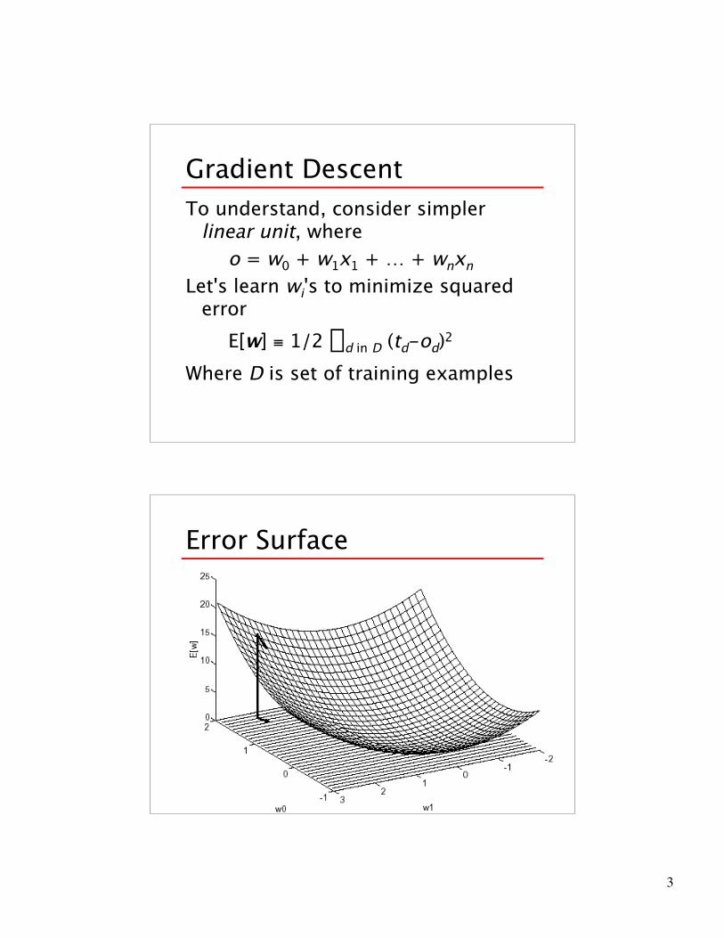
Gradient DescentTo understand, consider simpler

linear unit, whereo = w0 + w1x1 + … + wnxn

Let's learn wi's to minimize squarederror

E[w] ≡ 1/2 Sd in D (td-od)2Where D is set of training examples

Error Surface

4

Gradient DescentGradient—E [w] = [∂E/∂w0,∂E/∂w1,…,∂E/∂wn]

Training rule:Dw = -h —E [w]

in other words:Dwi = -h ∂E/∂wi

Gradient of Error∂E/∂wi

= ∂/∂wi 1/2 Sd (td-od)2= 1/2 Sd ∂/∂wi (td-od)2= 1/2 Sd 2 (td-od) ∂/∂wi (td-od)= Sd (td-od) ∂/∂wi (td-w xd)= Sd (td-od) (-xi,d)

5

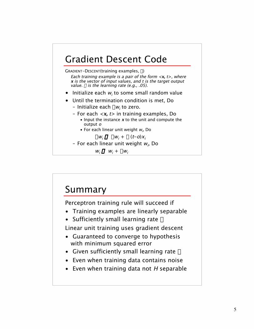
Gradient Descent CodeGRADIENT-DESCENT(training examples, h)

Each training example is a pair of the form <x, t>, wherex is the vector of input values, and t is the target outputvalue. h is the learning rate (e.g., .05).

• Initialize each wi to some small random value• Until the termination condition is met, Do

– Initialize each Dwi to zero.– For each <x, t> in training examples, Do

• Input the instance x to the unit and compute theoutput o

• For each linear unit weight wi, DoDwi ¨ Dwi + h (t-o)xi

– For each linear unit weight wi, Dowi ¨ wi + Dwi

SummaryPerceptron training rule will succeed if• Training examples are linearly separable• Sufficiently small learning rate hLinear unit training uses gradient descent• Guaranteed to converge to hypothesis

with minimum squared error• Given sufficiently small learning rate h• Even when training data contains noise• Even when training data not H separable

6

Stochastic Gradient DescentBatch mode Gradient Descent:Do until satisfied1. Compute the gradient —ED [w]2. w ¨ w - —ED [w]Incremental mode Gradient Descent:Do until satisfied• For each training example d in D

1. Compute the gradient —Ed [w]2. w ¨ w - —Ed [w]

More Stochastic Grad. Desc.ED[w] ≡ 1/2 Sd in D (td-od)2Ed [w] ≡ 1/2 (td-od)2Incremental Gradient Descent can

approximate Batch Gradient Descentarbitrarily closely if h set smallenough

7

Multilayer Networks

Decision Boundaries

8

Sigmoid Unit

s(x) is the sigmoid (s-like) function1/(1 + e-x)

Derivatives of SigmoidsNice property:

d s(x)/dx = s(x) (1-s(x))We can derive gradient decent rules to

train• One sigmoid unit• Multilayer networks of sigmoid

units Æ Backpropagation

9

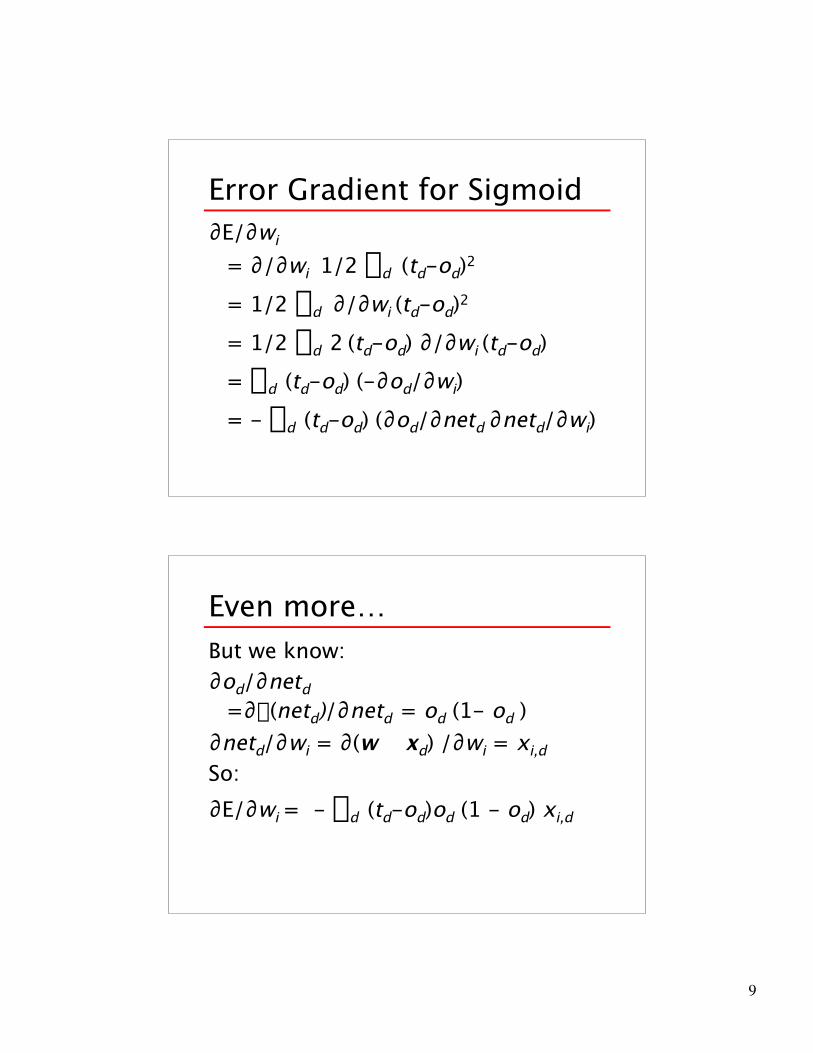
Error Gradient for Sigmoid∂E/∂wi

= ∂/∂wi 1/2 Sd (td-od)2= 1/2 Sd ∂/∂wi (td-od)2= 1/2 Sd 2 (td-od) ∂/∂wi (td-od)= Sd (td-od) (-∂od/∂wi)= - Sd (td-od) (∂od/∂netd ∂netd/∂wi)

Even more…But we know:∂od/∂netd

=∂s(netd)/∂netd = od (1- od )∂netd/∂wi = ∂(w · xd) /∂wi = xi,dSo:∂E/∂wi = - Sd (td-od)od (1 - od) xi,d

10

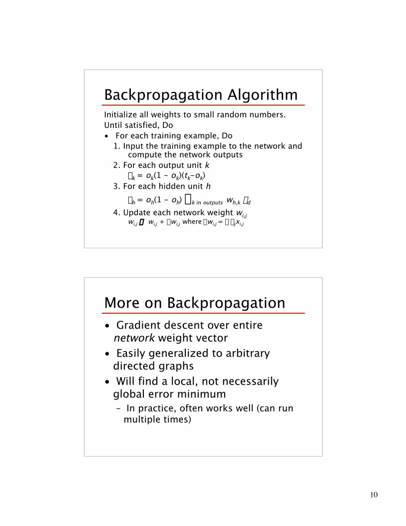
Backpropagation AlgorithmInitialize all weights to small random numbers.Until satisfied, Do• For each training example, Do

1. Input the training example to the network andcompute the network outputs

2. For each output unit kdk = ok(1 - ok)(tk-ok)

3. For each hidden unit h dh = oh(1 - oh) Sk in outputs wh,k dd

4. Update each network weight wi,jwi,j ¨ wi,j + Dwi,j where Dwi,j = h djxi,j

More on Backpropagation• Gradient descent over entire

network weight vector• Easily generalized to arbitrary

directed graphs• Will find a local, not necessarily

global error minimum– In practice, often works well (can run

multiple times)

11

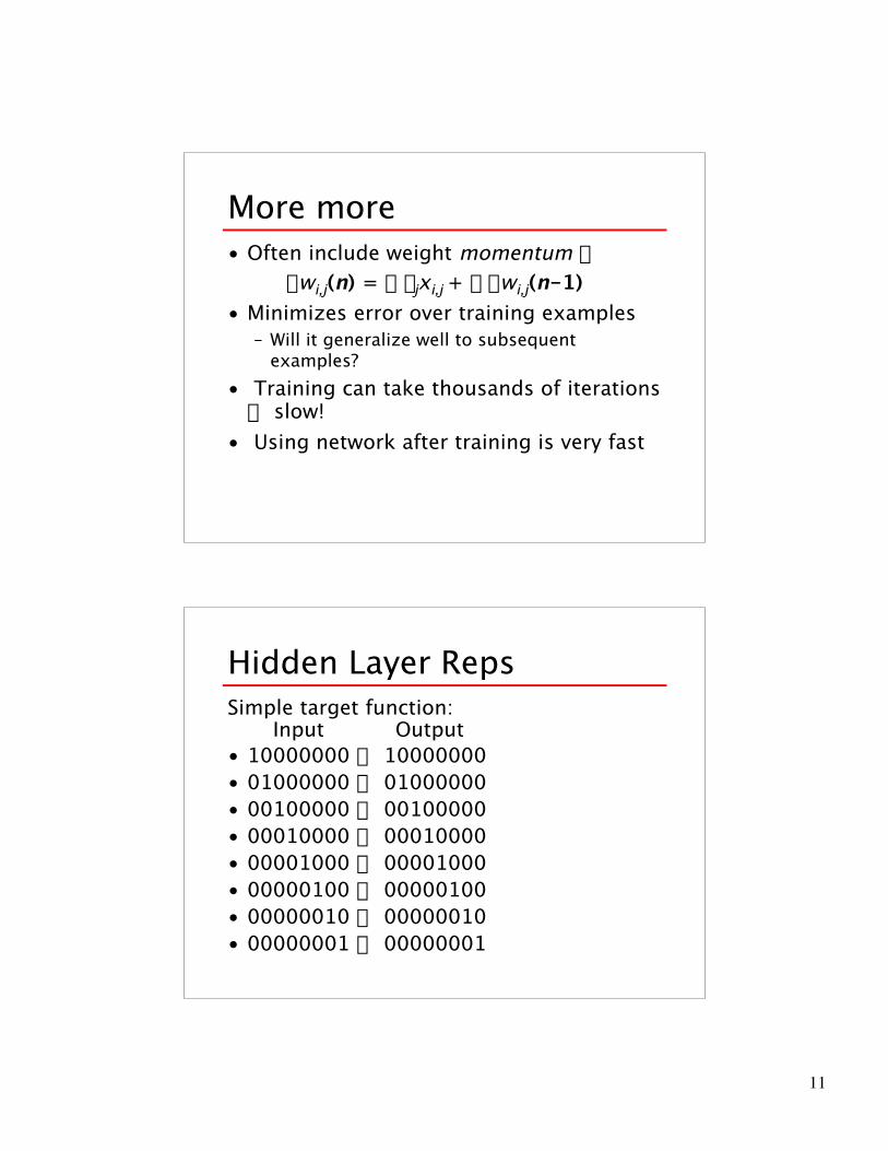
More more• Often include weight momentum a

Dwi,j(n) = h djxi,j + a Dwi,j(n-1)• Minimizes error over training examples

– Will it generalize well to subsequentexamples?

• Training can take thousands of iterationsÆ slow!

• Using network after training is very fast

Hidden Layer RepsSimple target function: Input Output• 10000000 Æ 10000000• 01000000 Æ 01000000• 00100000 Æ 00100000• 00010000 Æ 00010000• 00001000 Æ 00001000• 00000100 Æ 00000100• 00000010 Æ 00000010• 00000001 Æ 00000001

12

Autoencoder

Can the mapping be learned with this network??

Hidden Layer Rep. Input Hidden Values Output• 10000000 Æ .89 .04 .08 Æ 10000000• 01000000 Æ .01 .11 .88 Æ 01000000• 00100000 Æ .01 .97 .27 Æ 00100000• 00010000 Æ .99 .97 .71 Æ 00010000• 00001000 Æ .03 .05 .02 Æ 00001000• 00000100 Æ .22 .99 .99 Æ 00000100• 00000010 Æ .80 .01 .98 Æ 00000010• 00000001 Æ .60 .94 .01 Æ 00000001

13

Training

Training

14

Training

Convergence of BackpropGradient descent to some local

minimum• Perhaps not global minimum...• Add momentum• Stochastic gradient descent• Train multiple nets with different

initial weights

15

More on ConvergenceNature of convergence• Initialize weights near zero• Therefore, initial networks are

near-linear• Increasingly non-linear functions

possible as training progresses

Expressiveness of ANNsBoolean functions:• Every Boolean function can be

represented by network with singlehidden layer

• but might require exponential (innumber of inputs) hidden units

16

Real-valued FunctionsContinuous functions:• Every bounded continuous function can

be approximated, with arbitrarily smallerror, by network with one hidden layer[Cybenko 1989; Hornik et al. 1989]

• Any function can be approximated toarbitrary accuracy by a network with twohidden layers [Cybenko 1988].

Overfitting in ANNs (Ex. 1)

17

Overfitting in ANNs (Ex. 2)

When do you stop training?

Face Recognition

18

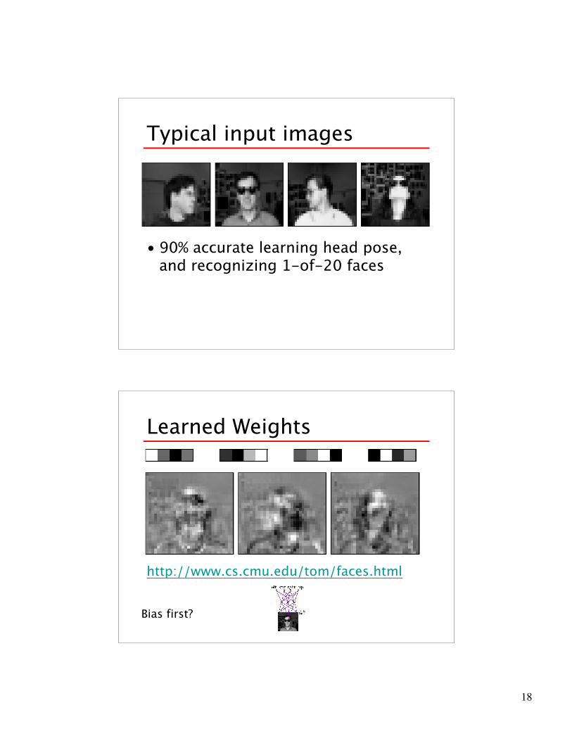
Typical input images

• 90% accurate learning head pose,and recognizing 1-of-20 faces

Learned Weights

http://www.cs.cmu.edu/tom/faces.html

Bias first?

19

Alternative Error FunctionsPenalize large weights:E(w) ≡ 1/2 Sd in D Sk in outputs (tkd-okd)2

+ g Sij wji2

Train on target slopes as well as values:

Tie together weights:• e.g., in phoneme recognition network

Recurrent Networks

20

Unfolding: BPTT