
Chapter 4 Design and Analysis of the Proposed Composite...
86
Chapter 4. Design and analysis of composite post and related structures 53 Chapter 4 Design and Analysis of the Proposed Composite Post and Related Structural Elements In the previous section, the analysis of the steel post was presented. The present section differs greatly from the previous in that the proposed composite post must be designed before any type of analysis treatment can be done. In relation to this project, the original steel post has a particular geometry, material, and boundary conditions which are unchangeable, that is to say this post has been designed previously and all that is required in this project is an analysis of the structure. This analysis brings the project up to the present point where the determined behavioural response is utilised in the initial design of the proposed composite post. The chapter defines the geometry of the composite post, its structural elements, and a number of laminate combination sub-models to be analysed. The analysis is carried out using the FEM with the behavioural response magnitudes of the original post, in particular displacement, being implemented as the constraints imposed on the proposed post model. The authenticity of the FEM model is confirmed by semi-analytic analyses which include CLT and a smeared approach. Additional loading scenarios are also analysed in the chapter while although conservative, they represent loading issues specific to the proposed structure’s service environment. Finally, a design and analysis of a steel resistant moment base is realised. The objective of this related structure is to provide the constrained boundary conditions necessary to enable the post to execute its service requirements. 4.1 Problem Data 4.1.1 Geometry While the overall geometrical constraints are maintained, the geometry of the proposed post differs slightly from the original steel geometrical configuration so as to incorporate general fabrication methods of structures made from composite materials. The original steel structure is composed of two U-section beams (UPN) fixed together by plates. The plates are connected by butt-welding. This specific geometry creates problems if it is to be directly applied in composite materials. A more efficient geometry in terms of fabrication and joining was
Transcript of Chapter 4 Design and Analysis of the Proposed Composite...

Chapter 4. Design and analysis of composite post and related structures 53
Chapter 4
Design and Analysis of the Proposed Composite
Post and Related Structural Elements
In the previous section, the analysis of the steel post was presented. The present section differs
greatly from the previous in that the proposed composite post must be designed before any
type of analysis treatment can be done. In relation to this project, the original steel post has a
particular geometry, material, and boundary conditions which are unchangeable, that is to say
this post has been designed previously and all that is required in this project is an analysis of the
structure. This analysis brings the project up to the present point where the determined
behavioural response is utilised in the initial design of the proposed composite post.
The chapter defines the geometry of the composite post, its structural elements, and a number
of laminate combination sub-models to be analysed. The analysis is carried out using the FEM
with the behavioural response magnitudes of the original post, in particular displacement,
being implemented as the constraints imposed on the proposed post model. The authenticity
of the FEM model is confirmed by semi-analytic analyses which include CLT and a smeared
approach. Additional loading scenarios are also analysed in the chapter while although
conservative, they represent loading issues specific to the proposed structure’s service
environment. Finally, a design and analysis of a steel resistant moment base is realised. The
objective of this related structure is to provide the constrained boundary conditions necessary
to enable the post to execute its service requirements.
4.1 Problem Data
4.1.1 Geometry
While the overall geometrical constraints are maintained, the geometry of the proposed post
differs slightly from the original steel geometrical configuration so as to incorporate general
fabrication methods of structures made from composite materials. The original steel structure
is composed of two U-section beams (UPN) fixed together by plates. The plates are connected
by butt-welding. This specific geometry creates problems if it is to be directly applied in
composite materials. A more efficient geometry in terms of fabrication and joining was

Chapter 4. Design and analysis of composite post and related structures
therefore examined and implemented in the composite model.
geometrical configurations presented in this project. The only difference geometrically between
the two is the inclusion of hole
from this, the overall dimensions are the same in both models.
Within each model there lies a second variation. Each model is split into two sub
are a result of distinct lamin
contains a ply mix of woven fibres (weave) and unidirectional fibres (tape) while the second
sub-model (B) in each model contains plies of unidirectional fibres only. These two different ply
types are described more extensively in Section 4.1.
schematic representation of the two different types of models and their subsequent variations
within due to different laminate composition. In total there are four post designs and will be
denoted by their number/letter comb
composed of laminates containing unidirectional fibre
Figure 4.1: Four different designs of proposed composite post
The new structure consists of four separate structural components
U-profile beams and two identic
through adhesion. The beam flanges are fixed to the inside of the plate surface and are aligned
along the plate edges so as to converg
the second model type are contained in the plate component (mechanized post
incorporated in the free surface
the UPNs. Figure 4.2 shows firstly the four components (including holes in plates of model 2)
separately but in their correct orientation
form the complete post. The diameters of the holes are contained within the area o
not fixed to the beam flanges and appropriately reduce along the leng
the top.
2 Model Types
of composite post and related structures
therefore examined and implemented in the composite model. In all, there are two types of
geometrical configurations presented in this project. The only difference geometrically between
the two is the inclusion of holes or cut-outs in the width of the post in one of the models. Apart
from this, the overall dimensions are the same in both models.
Within each model there lies a second variation. Each model is split into two sub
are a result of distinct laminate configurations for both. The first sub-
contains a ply mix of woven fibres (weave) and unidirectional fibres (tape) while the second
model (B) in each model contains plies of unidirectional fibres only. These two different ply
re extensively in Section 4.1.3 of Materials. Below
schematic representation of the two different types of models and their subsequent variations
within due to different laminate composition. In total there are four post designs and will be
denoted by their number/letter combination, e.g. 1B is the post structure
of laminates containing unidirectional fibres only.
: Four different designs of proposed composite post
of four separate structural components which include two identical
profile beams and two identical plates of varying width. The components
through adhesion. The beam flanges are fixed to the inside of the plate surface and are aligned
along the plate edges so as to converge towards the top of structure. The holes which define
the second model type are contained in the plate component (mechanized post
incorporated in the free surface of the plate, i.e. the plate surface area not directly bonded to
firstly the four components (including holes in plates of model 2)
separately but in their correct orientation and secondly the components joined together to
. The diameters of the holes are contained within the area o
not fixed to the beam flanges and appropriately reduce along the length of the post towards
1) No Holes
1A) Weave + Tape
1B) Tape
2) Holes
2A) Weave +Tape
2B) Tape
54
In all, there are two types of
geometrical configurations presented in this project. The only difference geometrically between
outs in the width of the post in one of the models. Apart
Within each model there lies a second variation. Each model is split into two sub-models which
-model (A) of the two
contains a ply mix of woven fibres (weave) and unidirectional fibres (tape) while the second
model (B) in each model contains plies of unidirectional fibres only. These two different ply
3 of Materials. Below in figure 4.1 is a
schematic representation of the two different types of models and their subsequent variations
within due to different laminate composition. In total there are four post designs and will be
st structure with no holes
: Four different designs of proposed composite post
which include two identical
components are fixed together
through adhesion. The beam flanges are fixed to the inside of the plate surface and are aligned
s the top of structure. The holes which define
the second model type are contained in the plate component (mechanized post-curing) and are
of the plate, i.e. the plate surface area not directly bonded to
firstly the four components (including holes in plates of model 2)
and secondly the components joined together to
. The diameters of the holes are contained within the area of the plate
th of the post towards
1A) Weave + Tape
1B) Tape
2A) Weave +Tape
2B) Tape

Chapter 4. Design and analysis of composite post and related structures 55
A box-type section for the structure was decided upon instead of using an open-type (I-type)
section as its sectional configuration have a more effective resistance to torsion than the open-
type section as all its parts at the periphery of the box section are connected to one another.
Secondly, while no torsional conditions are applied in the project data, the box section is a
design variable that is maintained from the original steel post structure.
Figure 4.2: Separate substructures and complete post
A detailed geometric representation of the structure is shown in figure 4.3. The thicknesses of
the UPNs and plate elements have been omitted as they vary with different types of layer
configuration of the laminate. In this report, there are three distinct types of composite
configurations examined. As with the original steel structure, the geometric sectional
boundaries are identical so as to incorporate the cantilever and the catenary elements without
making any additional adjustments at their connections. The structure stands at a height of 7 m
which is actually 1 m shorter than its steel counterpart. This is due to the distinct boundary
conditions of the two which are described in detail later. The structure’s width varies from 460
mm at its base to 200 mm at the top. The thickness of the post is 140 mm.

Chapter 4. Design and analysis of composite post and related structures 56
Figure 4.3: Dimensions of composite post structure
4.1.2 Boundary Conditions and Loads
The two moment cases of the original steel post outlined in Section 3.1.2 are generated by the
wind pressure exerted onto the post’s surface in directions perpendicular and parallel to the
rail line. The pressures calculated from this section for both load cases provide an approximate
representation of the wind loading that is also applied onto the free surface of the composite
post structure. The pressures for both cases are again outlined below in table 4.1, recalling that
the difference in magnitudes between both cases is assumed to be due to the additional
loading exerted by the catenary assembly in Case 1.

Chapter 4. Design and analysis of composite post and related structures 57
Pressure Load Perpendicular to line
(Case 1)
Parallel to line
(Case 2)
P (N/m2) 3072.886 2188.072
Table 4.1: Pressure P for cases 1 and 2
As outlined in the geometry, the proposed composite post differs from the original steel post in
terms of its method of fixation. While the original post of overall length of 8 m is embedded in a
concrete foundation of a depth of 1 m, the proposed post is instead fixed onto the top of this
same type of concrete pad by a steel moment resistant base as shown in figure 4.4. The overall
height of the proposed post is therefore reduced to 7 m with the bottom 200 mm fixed in the
moment resistant base. For simplification purposes of the composite model this bottom section
of 200 mm is treated as completely fixed, i.e. translations and rotations impeded. A separate
analysis of the combined base and post is carried out later in Section 4.8.
Figure 4.4: Composite post (blue) fixed to steel moment resistant base (grey)
As well as being the overall lighter structure of the two, the composite post with holes
experiences a reduced resultant force R for load Case 2, in comparison to the composite post
with no holes, due to its reduced surface area. However, this reduced surface area
consequently reduces the moment inertia (about the y-axis) and therefore its mechanical
resistance is negatively affected. This effect is analysed in more detail in the second part of
Section 4.1.4. As previously stated in Section 3.1.2, the additional loading effect due to the
catenary assembly is considered as a separate numerical analysis in Section 4.7.2.

Chapter 4. Design and analysis of composite post and related structures 58
4.1.3 Materials
The post is a composite based structure that is composed of two principal components, the
fibre and the matrix. The fibre component consists of a carbon based material. There are two
processes in which to fabricate the carbon fibre, they include the PAN (polyacrylonitrile) and
pitch process. The principal objective of the fibre component is to support approximately 70%
to 90% of the applied loading, and to provide mechanical resistance and stiffness to the
material. The matrix component consists of a polymeric resin which in this case is epoxy. The
objective of the epoxy is to give cohesion and maintain the fibre’s principal direction(s),
transmit loads to the fibres, protect the fibres from environmental degradation and provide
shear resistance between plies. There are two types of carbon/epoxy composite plies utilised in
the analysis depending on the model type, they are defined, with their thickness included, in
table 4.2 below.
Ply type Thickness (mm)
1 Woven fibres (weave fabric) 0.280
2 Unidirectional fibres (tape) 0.184
Table 4.2: Ply types and their thicknesses incorporated in laminates
The first is a carbon fibre weave which contains the same quantity of fibres in orthogonal
directions i.e. 0o and 90
o angles. The weave thereby gives equal mechanical resistance in the
orthogonal angles but consequently the maximum resistance that can be achieved is decreased.
The second type of composite utilised in the model a unidirectional fibre ply composite. The
unidirectional fibre provides a high mechanical resistance in one direction only of the ply or
lamina and an extremely limited resistance in the direction perpendicular to the fibre.
As previously outlined, sub-model A of both models is composed of a combination of woven
and unidirectional plies with the bulk of the structure to be composed principally of the weave
composite while the unidirectional composite is to be incorporated in areas/directions of high
tension and large displacements. Sub-model B of both models is composed solely of
unidirectional plies. To account for the limited transversal mechanical resistance of the
unidirectional ply, the laminate configuration requires off-axis and transversal orientation of
the ply to be included.
In the both types of composites utilised the resin introduction during ply fabrication is the
same, which is that the resin component is impregnated into the lamina in a fresh/uncured
state and therefore requires a system of curing to gain consistency [3], [9].

Chapter 4. Design and analysis of composite post and related structures 59
4.1.3.1 Elastic Properties
The material properties for both composites to be inputted in the model are orthotropic. The
state of plane stress in the ply causes the stress associated with the transversal direction to be
equal to zero ( 031233 === σσσ ) thereby reducing the associated properties in the
compliance matrix S. The relevant elastic properties for both composite orthotropic materials
are listed below in table 4.3. These values are typical elastic constants of carbon/epoxy-based
composites utilised in aeronautical applications and have been taken from an experimental and
numerical analysis of a mixed laminate (weave and tape) cylindrical stiffened composite panel
tested at the TEAMS facility in conjunction with the School of Engineering, University of Seville,
Spain. The elastic properties include: Young’s Modulus in the both in-plane orthogonal
directions (E11 and E22); the shear modulus (G12); and Poisson’s ratio (v12). Both the longitudinal
and transversal elastic properties influence the total stiffness of the composite. The elastic
properties for the two types of composites utilised in the project are as follows:
Property Weave Fabric
Composite Ply
Unidirectional Tape
Composite Ply
E11 (GPa) 61 131
E22 (GPa) 61 9.75
G12 (GPa) 4.9 4.65
G13 (GPa) 4.9 4.65
G23 (GPa) 3 3
v12 0.05 0.3
Table 4.3: Elastic properties of weave and unidirectional composites
4.1.3.2 Mechanical Strength Properties
The strength of the composite takes into account longitudinal, transversal and shear strengths.
These mechanical strength properties include tensile resistance in the direction of the fibres XT,
resistance to compression in the direction of the fibres XC, tensile resistance in the transverse
direction to the fibres YT, and resistance to compression in the transverse direction to the fibres
YC and shear resistance S. These mechanical strength properties, supported by a selected failure
criterion, will allow for the prediction of failure in the structure. There are three predefined
failure criteria in the ANSYS program which include Maximum Strain, Maximum Stress and Tsai-
Wu Failure Criterion. Additional types of failure criteria will be later proposed by the author
through the application of a macro-written code applicable to the ANSYS program. Table 4.4
gives the mechanical strength values for ply types.

Chapter 4. Design and analysis of composite post and related structures 60
Properties Weave Fabric
Composite
Unidirectional Fibre
Composite
MPa MPa
XT 460 2220
XC 435 1300
YT 460 60
YC 435 240
S 155 108
Table 4.4: Mechanical strength properties of weave and unidirectional composites
4.1.4 Ply Orientation and Laminate Design
Unlike materials with isotropic characteristics, composites can include an additional design
variable which is ply orientation. The elastic and mechanical properties outlined above clearly
indicate that the stiffness and strength of a composite depend on the orientation of the fibres.
A laminate’s mechanical capabilities can be varied to account for direction of loading by
changing the fibre orientation of the plies while not affecting the overall thickness of the
laminate. With the provision of using stiffeners in a structure, a higher modulus of elasticity can
be applied to the flange part of the stiffener by concentrating the fibre direction of the plies
along its longitude. It is therefore possible to tailor a laminate to the specific conditions applied
to the problem.
As it has been stated before, the project presents the results of two general types of laminates:
The first is a combination of woven and unidirectional plies; and the second is a laminate
containing unidirectional plies only. The difference in structural behaviour between the two
laminate types is directly associated to the type of ply used, quantity and its orientation.
Both of the types of composites utilised have their own application purposes. The woven fabric
allows easy processing as it is produced in prepreg laminas and can be more readily applied and
wrapped into relatively complex shapes than the unidirectional composite. The matrix of the
unidirectional composite tends to separate from the fibre in its weak transversal direction when
applied to irregular shaped surfaces. The main advantage of the unidirectional fibre composite
is that it is utilised in the directions of large stresses and displacements allowing for maximum
manipulation of strength in the most critically anticipated directions. A number of plies are
orientated off the global axes; these include orientations of 45o and -45
o which increases the
shear strength of the laminate and reduces torsion within the structure.
The configurations of each plate and UPN component for the two models are shown
respectively below in table 4.5 and table 4.6. Within the laminate configuration, each ply’s
orientation is described by the angle (in degrees) written in normal size font. Angles that are

Chapter 4. Design and analysis of composite post and related structures 61
underlined define the weave ply while the remaining angles not underlined define the tape ply.
The subscript number relates to the multiple of the number of plies defined within the bracket
pair. Finally, subscript s implies that the configuration is symmetric.
It is worth noting at this point that all laminates shown are symmetric which implies a reduction
in the number of independent elastic constants from 21 which characterises anisotropic
materials to 13 independent constants which is termed as a monoclinic laminate material. From
viewing the configurations of the laminates in sub-models A (weave + tape) for both models, it
is evident that no 90o plies have been defined in the configuration. Mechanical resistance in the
transversal direction is gained through inclusion of the weave ply as it gives equal mechanical
resistance in the orthogonal angles so by only defining the 0o, it is implied that equal resistance
is attained in its orthogonal angle, which in this instance is 90o. Angled plies of +45
o and -45
o are
defined in equal quantities so as to maintain equivalent proportions of each angle in the
laminate.
On a final observation of the configurations, it is worth highlighting that only the unidirectional
ply is orientated at +/-45o in all laminates, this is due to a fabrication constraint imposed on the
weave ply. During lamination, the post’s substantial length of 7 m causes an issue of ply join-up.
At an angle of 45o, a number of plies are required to be laid-up together at their edges in order
to completely cover the laminate. Plies cannot be jointly laid-up together end to end through
the direction of the fibre as this creates a discontinuity and stress are not transferred through
the entire layer. For this particular reason, the weave ply cannot be jointly laid-up as one of its
orthogonal axes of mechanical resistance would be rendered discontinuous. See Section 5.2 on
the lay-up process for additional information.
Model 1 Substructure Ply Configuration
A Weave + Tape Plate [(0/0)2/(0/45/0/-45)3/(0)2]s
Beam [(0/0)2/(0/45/0/-45)4/(0/0)2]s
B Tape Plate [(0/45/90/-45/(0)4)2]s
Beam [(0/45/90/-45/(0)4/(0/45/90/-45)2/(0)6]s
Table 4.5: Laminate configuration for post with no holes (Model 1)
Model 2 Substructure Ply Configuration
A Weave + Tape Plate [(0/0)4/(0/45/0/-45)3]s
Beam [(0/0)4/(0/45/0/-45)4/(0/0)2]s
B Tape Plate [(0/45/90/-45/(04))2/(0)2]s
Beam [(0/45/90/-45/(04))2/(0/45/90/-45)2/(0)8]s
Table 4.6: Laminate configuration for post with holes (Model 2)

Chapter 4. Design and analysis of composite post and related structures 62
Tables 4.7 and 4.8 presents a summarised view of the design considerations for the laminate
configurations including overall percentage thickness of both the plate and beam components
and percentage of fibres orientated off-axis, or at +/-45o. In the cases of combined weave and
tape laminates, the percentage off-axis laminates is not considered by the number of plies but
rather by the thickness of such orientated fibres. Other data presented include the number of
plies and thickness for each laminate.
The objective of the laminate configuration design is to maintain equivalent proportions (%
thickness and % +/-45o) between both sub-models (A and B) for each model (1 and 2) while also
maintaining equivalent magnitudes of the critical design control, which in this project is the
maximum displacement permitted. While the variation in the quantity of plies/thickness
between sub-models A and B is a result of the different mechanical resistance provoked by
distinct ply combinations, proportionally both sub-models are maintained approximately the
same. In all models, the overall percentage thickness of the plate and the beam are
approximately 42-43% and 57-58%, respectively. A slight difference in the proportion of +/-45o
occurs between both models but is maintained relatively equal for the sub-models A and B. The
slight difference in proportions arises due to the requirement of maintaining +45o and -45
o at
equal quantities while the total number of plies in the laminate varies between both models.
Model 1 Substructure
No. of
plies
Thickness
(mm)
Overall %
Thickness % +/-45o
A Weave + Tape Plate 36 8.352 43 27
Beam 48 11.136 57 26.4
B Tape Plate 32 5.888 42 25
Beam 44 8.096 58 27.3
Table 4.7: Laminate design of post in Model 1
Model 2 Substructure
No. of
plies
Thickness
(mm)
Overall %
Thickness % +/-45o
A Weave + Tape Plate 40 9.28 42 23.8
Beam 56 12.992 58 22.6
B Tape Plate 36 6.624 43 22.2
Beam 48 8.832 57 25
Table 4.8: Laminate design of post in Model 2

Chapter 4. Design and analysis of composite post and related structures 63
4.2 Finite Element Model
The following section relates to the most efficient approach, as regarded by the author, to
create an accurate representation of the newly designed post structure in composite materials.
The following approach considers the most suitable element type, meshing requirements and
application of boundary conditions. Due to the orthotropic nature of the composite materials
analysed in this model and the complexity of the geometry, issues encountered with ply
orientation are emphasised extensively in the following.
4.2.1 Element Type
As in the case of the original structure, ANSYS is the preferred finite element program to be
used for modelling. One type of element is employed in this composite model, namely
SHELL181. Shell elements are designed to efficiently model thin structures. Structures
fabricated from composite materials by stacking methods of plies to create laminates are well
defined by shell elements. The SHELL181 element is a 4-node finite strain shell which is suitable
for analyzing thin to moderately thick shell structures. The element contains six degrees of
freedom which include translations in the x, y and z directions, and rotations about the x, y and
z-axes. Figure 4.5 shows the quadrilateral element with its coordinate direction with respect to
the configuration of the nodes (i, j, k, l). The coordinate system is directly related to the
configuration of the nodes where the z-axes is positive and transversal in an element when the
nodes are defined in an anti-clockwise manner, commencing at node i and moving out from the
x-axes towards the subsequent node j [8].
Figure 4.5: 4-node SHELL181 element
A number of elemental key options settings utilised in this model include applying a full
integration analysis (KEYOPT(3) = 2). This option is recommended as it is highly accurate (even
with coarse meshes) in that its application is well suited to cantilever-type problems which are
dominated by in-plane bending. The second key option setting utilised for this element stores

Chapter 4. Design and analysis of composite post and related structures 64
data for top and bottom for all layers in the laminate (KEYOPT(8) = 1). This permits the user to
obtain more accurate interlaminar results (e.g. stresses and strains) caused by different ply
types and orientations. Data for a specific layer is attained by calling on that layer through the
LAYER command. In relation to this project and briefly outlined in its objectives, this key option
setting enables the author to apply any type of desired failure criteria created in macro-style
parametric language (APDL), contained in the ANSYS program. This process is described in
detail later in Section 4.4. A typical laminate section with distinct interlaminar stress results (σx)
is shown in figure 4.6.
Figure 4.6: Interlaminar stress distribution through laminate section
4.2.2 Model Development Method
The complete post structure is divided essentially into four elemental sub-structures which
include two U-profile beams and two plates joined to the flanges of the beams as shown
previously in figure 1. The model is further subdivided into planar areas as shown in figure 4.7
which are themselves defined by keypoints (KP), lines (L) and areas (AL). For ease of analysis,
the plate area and to the flange area of the beam which are considered adhesively joined
together are considered unique and as one area. As a result, the laminate configuration at this
new unified area includes the laminate configuration of the plate plus the laminate
configuration of the flange.
Laminate Thickness

Chapter 4. Design and analysis of composite post and related structures 65
Figure 4.7: Post segment showing separated planar areas for lamination
The local coordinate system (LOCAL) defines the ply orientation of the laminate in question
with its relevant capabilities shown in figure 4.9. The origin of the local coordinate system is
defined by three points on the global Cartesian coordinate system and its orientation through
rotation of Euler angles. This permits each area to orientate the direction of the composite
fibres independently. Each area is meshed individually or collectively depending on whether or
not two or more areas share (1) the same configuration and (2) orientation. Before meshing of
the area, elemental attributes need to be assigned to that area and are done so by the AATT
command. From here the section information is associated with a section ID number through
the SECTYPE command which also defines the type of element (SHELL) and the name to be
given to that particular section, e.g. the first constructed area is ‘AREA1’. The geometry data
describing this section type is defined by the SECDATA command. It describes the lamina
configuration of the section by the thickness of each shell layer, material type and the angle (in
degrees) of the already-defined local coordinate system of the layer element.
A simplified sketch of the cross section of the structure is shown below figure 4.8. In total, there
are 8 planar areas that make up the outer boundary of the structure which highlighted in red in
the figure below. Their dimensions are equivalent to those of the original steel post, thereby
maintaining the same profile as has been outlined as a project constraint. From this, lamination
of all areas occurs from the areas surface towards the centroide of the cross section. As a
result, each section’s defined shell layers or configuration originates on the plane marked in red
and advances or stacks up in accordance to the sections own local coordinate system. This
method of lay-up is achieved by offsetting each section to the origin of their local z-axis through
the SECOFFSET command. Note that the SECOFFSET command is determined by the node
orientation of the element (i, j, k, l).

Chapter 4. Design and analysis of composite post and related structures 66
Figure 4.8: Section of structure with individual sections according to lamina lay-up direction
Orientation issues arise when attempting to represent laminates in a 3-D model. An example of
this is incurred with the orientation of a single layer about the UPN beam section. As described
in Section 5.5.2 of fabrication, the plies of the beam are laminated onto and around a suitable
mould profile. Three planar surface areas of the mould are to be covered by the layer. Figure
4.9 shows the layer and its fibre orientation before and after lamination. Before lamination and
in the first image, one local coordinate system defines the complet layer. In order to maintain
fibre orientation throughout lamination of a single layer around the three planar surfaces of the
mould the layer needs to be subdived into same number of local axes as the amount of
distinctly orientated planar axes, and in this case are three axes which are shown in the second
image of figure 4.9. Each of the three local coordinate systems are different and are defined as
so through the LOCAL command. While attention is required in defining the local coordinates,
the ply configuration or stacking sequence for the three laminates remain the same.
A complication arises in the stacking sequence due to the simplification of the unique surface
defined earlier between the plate area and beam flange adhered together. Taking the example
in bottom figure again, the top local coordinate system (x1, y1, z1) equivalent to the coordinate
system for the combined top flange/plate area defines this laminate configuration adequately.
However, the combined bottom flange/plate area becomes problematic in that the flange
configuration is adequately defined by the local coordinate system (x3, y3, z3) while the plate
configuration is not. The orientation of the fibres in top and bottom areas of the third image
describes issue. According to both sets of local coordinates in these areas (1 and 3), if an
abitrary layer is defined the same for both plate areas the fibre orientation would be opposite
to each other on the global axes as clearly evident in the final image of figure 7. To overcome
this event, the plate stacking of off-axis plies must be altered by 90o. For example, if a layer in
both the top and bottom plate is orientated 45o on the global axes the top layer, with local
coordinate system (x1, y1, z1), is defined at 45o while the bottom layer is defined as -45
o in
relation to its appropriate local coordinate system (x3, y3, z3).

Chapter 4. Design and analysis of composite post and related structures 67
Figure 4.9: Fibre orientation in laminated UPN beam
In relation to meshing of the structure, both U-profile beams are regular in shape and their
areas that make up the sub-structure are mapped meshed (forming straight-sided elements)
with a specific number of divisions made on the selected lines. In relation plate structures in
Model 2 where holes are incorporated in the plates, meshing requirements are more
specialised. As shown previously in figure 4.7 and below in figure 4.8, the plate components are
divided into 3 areas: 2 of which coincide with the area of the beam flange (blue), and the third
is the remaining area between the two beam flanges (green). This third area shares the same
line number with the two bordering flange/plate areas and thus is divided into the same
number of elements in its longitude so that boundary nodes between the 3 plate areas
Chapter 4. Design and analysis of composite post and related structures 68
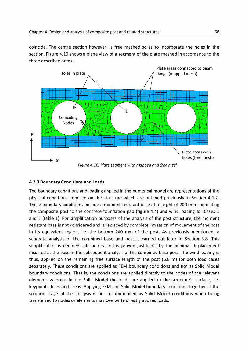
coincide. The centre section however, is free meshed so as to incorporate the holes in the
section. Figure 4.10 shows a plane view of a segment of the plate meshed in accordance to the
three described areas.
Figure 4.10: Plate segment with mapped and free mesh
4.2.3 Boundary Conditions and Loads
The boundary conditions and loading applied in the numerical model are representations of the
physical conditions imposed on the structure which are outlined previously in Section 4.1.2.
These boundary conditions include a moment resistant base at a height of 200 mm connecting
the composite post to the concrete foundation pad (figure 4.4) and wind loading for Cases 1
and 2 (table 1). For simplification purposes of the analysis of the post structure, the moment
resistant base is not considered and is replaced by complete limitation of movement of the post
in its equivalent region, i.e. the bottom 200 mm of the post. As previously mentioned, a
separate analysis of the combined base and post is carried out later in Section 3.8. This
simplification is deemed satisfactory and is proven justifiable by the minimal displacement
incurred at the base in the subsequent analysis of the combined base-post. The wind loading is
thus, applied on the remaining free surface length of the post (6.8 m) for both load cases
separately. These conditions are applied as FEM boundary conditions and not as Solid Model
boundary conditions. That is, the conditions are applied directly to the nodes of the relevant
elements whereas in the Solid Model the loads are applied to the structure’s surface, i.e.
keypoints, lines and areas. Applying FEM and Solid Model boundary conditions together at the
solution stage of the analysis is not recommended as Solid Model conditions when being
transferred to nodes or elements may overwrite directly applied loads.
Coinciding
Nodes
Plate areas connected to beam
flange (mapped mesh)
Plate areas with
holes (free mesh)
Holes in plate
Chapter 4. Design and analysis of composite post and related structures 69
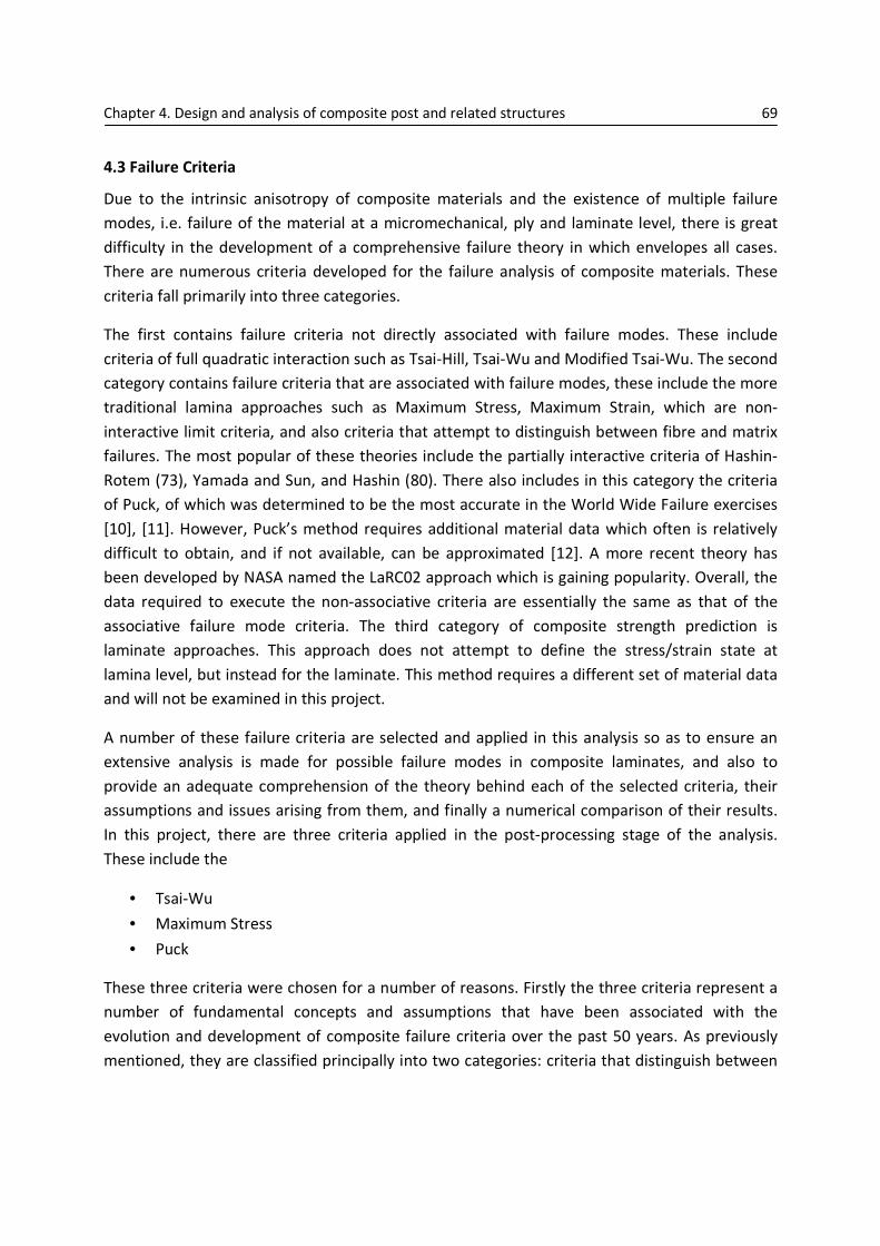
4.3 Failure Criteria
Due to the intrinsic anisotropy of composite materials and the existence of multiple failure
modes, i.e. failure of the material at a micromechanical, ply and laminate level, there is great
difficulty in the development of a comprehensive failure theory in which envelopes all cases.
There are numerous criteria developed for the failure analysis of composite materials. These
criteria fall primarily into three categories.
The first contains failure criteria not directly associated with failure modes. These include
criteria of full quadratic interaction such as Tsai-Hill, Tsai-Wu and Modified Tsai-Wu. The second
category contains failure criteria that are associated with failure modes, these include the more
traditional lamina approaches such as Maximum Stress, Maximum Strain, which are non-
interactive limit criteria, and also criteria that attempt to distinguish between fibre and matrix
failures. The most popular of these theories include the partially interactive criteria of Hashin-
Rotem (73), Yamada and Sun, and Hashin (80). There also includes in this category the criteria
of Puck, of which was determined to be the most accurate in the World Wide Failure exercises
[10], [11]. However, Puck’s method requires additional material data which often is relatively
difficult to obtain, and if not available, can be approximated [12]. A more recent theory has
been developed by NASA named the LaRC02 approach which is gaining popularity. Overall, the
data required to execute the non-associative criteria are essentially the same as that of the
associative failure mode criteria. The third category of composite strength prediction is
laminate approaches. This approach does not attempt to define the stress/strain state at
lamina level, but instead for the laminate. This method requires a different set of material data
and will not be examined in this project.
A number of these failure criteria are selected and applied in this analysis so as to ensure an
extensive analysis is made for possible failure modes in composite laminates, and also to
provide an adequate comprehension of the theory behind each of the selected criteria, their
assumptions and issues arising from them, and finally a numerical comparison of their results.
In this project, there are three criteria applied in the post-processing stage of the analysis.
These include the
• Tsai-Wu
• Maximum Stress
• Puck
These three criteria were chosen for a number of reasons. Firstly the three criteria represent a
number of fundamental concepts and assumptions that have been associated with the
evolution and development of composite failure criteria over the past 50 years. As previously
mentioned, they are classified principally into two categories: criteria that distinguish between

Chapter 4. Design and analysis of composite post and related structures
fibre failure and matrix failure (direct failure mode) and those that do
failure criteria directly associated with failure modes can be sub
categories: interactive and non
types is the existence (or non
and the influence of the transversal stress component for
describes the formation of the discussed categories and given are the criteria associated with
each type.
Figure 4.11: Categorisation of failure criteria applied in analysis
The second for choosing the above criteria is due to the presence of two types of composite
plies utilised in the design of the struc
(tape) composites. Issues arise with determining an appropriate failure criterion for each of the
two ply types. For instance, the direct
the application to unidirectional composites and not for woven
may therefore be called into question with the application of this criterion for the analysis of
the mixed ply laminates of M
for the application to the wove
criterion of Tsai-Wu [13].
The final reason for choosing these particular criteria is down to the discretion of the author.
The high accuracy of the Puck criterion in the World Wide Exercise a
Maximum Stress criterion in FEM commercial programs and industry contributed to these
criteria inclusion.
In this post-processing analysis of the project, the above criteria are executed by two different
methods. They include analysis through
• Predefined criteria in ANSYS
• Macro-style parametric language in ANSYS (APDL)
Failure Mode
(Criterion)
of composite post and related structures
fibre failure and matrix failure (direct failure mode) and those that do
failure criteria directly associated with failure modes can be sub-divided further into two
categories: interactive and non-interactive limit criteria. The difference between these two
types is the existence (or non-existence) of association between in-plane stress components
and the influence of the transversal stress component for a particular failure mode. Figure 4.11
describes the formation of the discussed categories and given are the criteria associated with
: Categorisation of failure criteria applied in analysis
The second for choosing the above criteria is due to the presence of two types of composite
plies utilised in the design of the structure, namely woven fibre (weave) and unidirectional fibre
pe) composites. Issues arise with determining an appropriate failure criterion for each of the
two ply types. For instance, the direct-interactive criterion of Puck was originally developed for
the application to unidirectional composites and not for woven composites. Accuracy of results
may therefore be called into question with the application of this criterion for the analysis of
odels 1B and 2B. Of the three presented, the criterion most suited
for the application to the woven fibre (in-plane stress) is the non-direct, fully inter
The final reason for choosing these particular criteria is down to the discretion of the author.
The high accuracy of the Puck criterion in the World Wide Exercise and the extensive use of the
Maximum Stress criterion in FEM commercial programs and industry contributed to these
processing analysis of the project, the above criteria are executed by two different
alysis through
Predefined criteria in ANSYS
style parametric language in ANSYS (APDL)
Failure Mode
Non-Direct
(Tsai-Wu)
Direct
Non-Interactive
(Max. Stress)
Interactive
(Puck)
70
fibre failure and matrix failure (direct failure mode) and those that do not (non-direct). The
divided further into two
interactive limit criteria. The difference between these two
plane stress components
a particular failure mode. Figure 4.11
describes the formation of the discussed categories and given are the criteria associated with
: Categorisation of failure criteria applied in analysis
The second for choosing the above criteria is due to the presence of two types of composite
) and unidirectional fibre
pe) composites. Issues arise with determining an appropriate failure criterion for each of the
interactive criterion of Puck was originally developed for
composites. Accuracy of results
may therefore be called into question with the application of this criterion for the analysis of
odels 1B and 2B. Of the three presented, the criterion most suited
direct, fully interactive
The final reason for choosing these particular criteria is down to the discretion of the author.
nd the extensive use of the
Maximum Stress criterion in FEM commercial programs and industry contributed to these
processing analysis of the project, the above criteria are executed by two different
Interactive
(Max. Stress)
Interactive
(Puck)
Chapter 4. Design and analysis of composite post and related structures 71
Of the three failure criteria to be applied in the analysis only the Maximum Stress and Tsai-Wu
criteria are readily available in the ANSYS FEM program. As a result, the third criterion (Puck) is
written as a macro file in APDL (ANSYS Parametric Design Language) and is executed in the
post-processing stage of the analysis. As stated previously, this parametric script coding is
described in detail in Section 4.4. For validity purposes of the macro-written criteria, the
Maximum Stress and Tsai-Wu criteria are also written in APDL and compared with failure
results of the predefined equivalent criteria in ANSYS.
All failure criteria results are presented as failure index values where a value greater or equal to
one signifies failure.
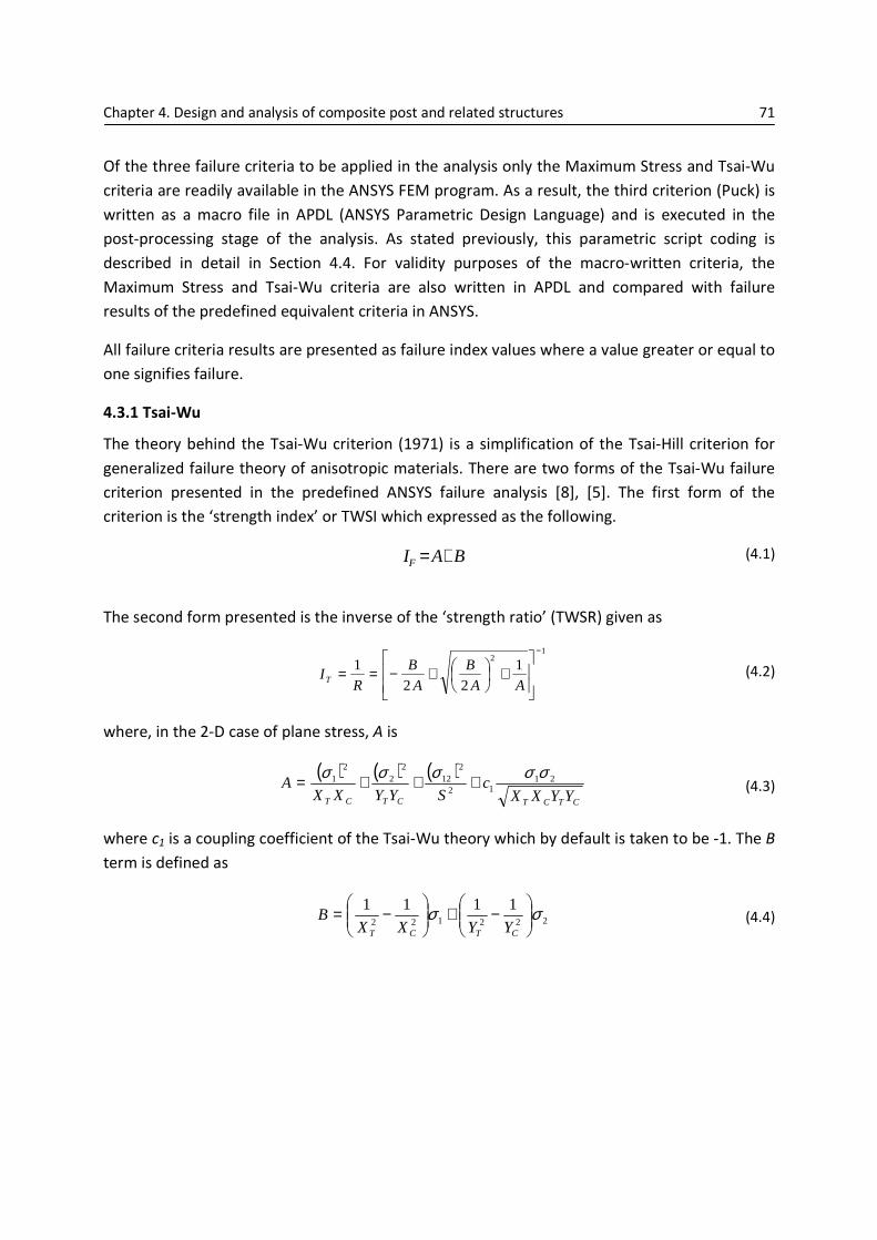
4.3.1 Tsai-Wu
The theory behind the Tsai-Wu criterion (1971) is a simplification of the Tsai-Hill criterion for
generalized failure theory of anisotropic materials. There are two forms of the Tsai-Wu failure
criterion presented in the predefined ANSYS failure analysis [8], [5]. The first form of the
criterion is the ‘strength index’ or TWSI which expressed as the following.
BAIF += (4.1)
The second form presented is the inverse of the ‘strength ratio’ (TWSR) given as
12
122
1−
+
+−==AA
B
A
B
RIT
(4.2)
where, in the 2-D case of plane stress, A is
( ) ( ) ( )
CTCTCTCT YYXXc
SYYXXA 21
12
212
22
21 σσσσσ +++= (4.3)
where c1 is a coupling coefficient of the Tsai-Wu theory which by default is taken to be -1. The B
term is defined as
222122
1111 σσ
−+
−=
CTCT YYXXB (4.4)

Chapter 4. Design and analysis of composite post and related structures 72
4.3.2 Maximum Stress
As previously mentioned, the maximum stress criterion does not consider any interaction
between stress/strains acting in the lamina and dictates failure to occur when the stress in any
direction exceeds the strength in that direction. As a result, this type of criterion under-predicts
the strength when combined in-plane stresses are acting on the composite. This type of
criterion is a simple, straightforward way to predict failure of composites. This more traditional
criterion predicts no material fracture, for a state of tension, occurs if:
TX<11σ ( )011≥σ (4.5a)
TY<22σ ( )022 ≥σ (4.6b)
S<12σ (4.6c)
And for a state of compression if:
CX<11σ ( )011<σ (4.7a)
CY<22σ ( )022<σ (4.7b)
Where one or more of the inequalities are not met fracture occurs in the material according to
the mechanism associated to that equation in which the inequality has not been met [5].
4.3.3 Puck
The Puck failure criterion is one type of criterion that is associated with failure modes. The
criterion distinguishes between fibre failure (FF) and inter-fibre failure (IFF). In relation IFF or
failure of the matrix, the in-plane failure parallel to the fibres is governed by the three stress
vector components associated with that plane which include the normal stress acting on the
plane, and two planar stresses, one acting parallel and the other perpendicular to the fibre. The
criterion proposes that the two shear stresses always promote fracture, while the normal stress
only promotes fracture if it is in a traction state and has the adverse effect in compression, i.e.
it impedes fracture [12].
IFF contains three distinct modes of failure: mode A is when perpendicular transversal cracks
appear in the ply under transversal tensile stress with or without in-plane shear stress; Mode B
also implies transversal cracks, but are a caused by in-plane shear stress with small transverse
compression stress; and finally Mode C denotes oblique cracks onset (typically of angle 53o in

Chapter 4. Design and analysis of composite post and related structures 73
carbon/epoxy composites) when the material is under significant transversal compression. The
FF yields one failure index which assumes that fibre failure only depends on longitudinal
tension [14]. It is defined as
TX<11σ ( )011≥σ (4.8a)
CX<11σ
( )011<σ (4.8b)
The three failure modes in the IFF imply that it yields three separate index failures. The
particular IFF mode to be activated for analysis depends on the stress state of the lamina in
question. For instance, mode A is activated if the transversal stress is positive. It is expressed as
11 212
2
2
1212 =+
−+
Sp
YS
Yp
S TT
T
T σσσ
( )022 ≥σ (4.9)
where T
p12 is the slope of the failure curve for 022≥σ at the point 022=σ , also known as a
fitting parameter. Without experimental values, the parameter is assumed to be 0.3 which is
representative of carbon based composites. In relation to negative transverse stress 022<σ ,
either Mode B or Mode C is activated, depending on the relationship between in-plane shear
stress and transversal stress. The selection of either mode is defined by the limit of the relation
YA/SA where
−+= 121
2 1212 S
Yp
p
SY C
A C
C
(4.10)
C
pSS A 221+= (4.11)
and
A
A
S
Ypp
CC 122 = (4.12)
where C
p12 is another fitting parameter but which corresponds to the interlaminar shear
strength S. A value of 0.2 is selected to represent this parameter [14]. The failure index and its
limitation YA/SA for Mode B are defined as
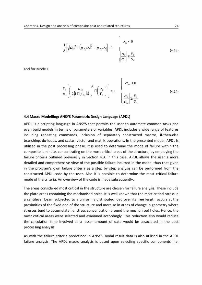
Chapter 4. Design and analysis of composite post and related structures 74
( ) 11
2122
2122
12 =
++ σσσ
CCpp
S
≤
<
A
A
S
Y
12
2
22 0
σσ
σ
(4.13)
and for Mode C
( ) 112
2
2
2
2
12
2
=
+
+−
C
C
YSp
Y
C
σσσ
≥
<
A
A
S
Y
12
2
22 0
σσ
σ
(4.14)
4.4 Macro Modelling: ANSYS Parametric Design Language (APDL)
APDL is a scripting language in ANSYS that permits the user to automate common tasks and
even build models in terms of parameters or variables. APDL includes a wide range of features
including repeating commands, inclusion of separately constructed macros, if-then-else
branching, do-loops, and scalar, vector and matrix operations. In the presented model, APDL is
utilised in the post processing phase. It is used to determine the mode of failure within the
composite laminate, concentrating on the most critical areas of the structure, by employing the
failure criteria outlined previously in Section 4.3. In this case, APDL allows the user a more
detailed and comprehensive view of the possible failure incurred in the model than that given
in the program’s own failure criteria as a step by step analysis can be performed from the
constructed APDL code by the user. Also it is possible to determine the most critical failure
mode of the criteria. An overview of the code is made subsequently.
The areas considered most critical in the structure are chosen for failure analysis. These include
the plate areas containing the mechanised holes. It is well known that the most critical stress in
a cantilever beam subjected to a uniformly distributed load over its free length occurs at the
proximities of the fixed end of the structure and more so in areas of change in geometry where
stresses tend to accumulate i.e. stress concentration around the mechanised holes. Hence, the
most critical areas were selected and examined accordingly. This reduction also would reduce
the calculation time involved as a lesser amount of data would be associated in the post
processing analysis.
As with the failure criteria predefined in ANSYS, nodal result data is also utilised in the APDL
failure analysis. The APDL macro analysis is based upon selecting specific components (i.e.
Chapter 4. Design and analysis of composite post and related structures 75
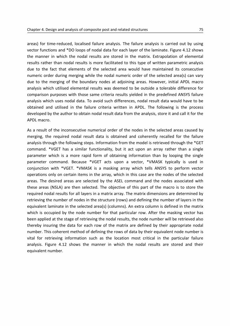
areas) for time-reduced, localised failure analysis. The failure analysis is carried out by using
vector functions and *DO loops of nodal data for each layer of the laminate. Figure 4.12 shows
the manner in which the nodal results are stored in the matrix. Extrapolation of elemental
results rather than nodal results is more facilitated to this type of written parametric analysis
due to the fact that elements of the selected area would have maintained its consecutive
numeric order during merging while the nodal numeric order of the selected area(s) can vary
due to the merging of the boundary nodes at adjoining areas. However, initial APDL macro
analysis which utilised elemental results was deemed to be outside a tolerable difference for
comparison purposes with those same criteria results yielded in the predefined ANSYS failure
analysis which uses nodal data. To avoid such differences, nodal result data would have to be
obtained and utilised in the failure criteria written in APDL. The following is the process
developed by the author to obtain nodal result data from the analysis, store it and call it for the
APDL macro.
As a result of the inconsecutive numerical order of the nodes in the selected areas caused by
merging, the required nodal result data is obtained and coherently recalled for the failure
analysis through the following steps. Information from the model is retrieved through the *GET
command. *VGET has a similar functionality, but it act upon an array rather than a single
parameter which is a more rapid form of obtaining information than by looping the single
parameter command. Because *VGET acts upon a vector, *VMASK typically is used in
conjunction with *VGET. *VMASK is a masking array which tells ANSYS to perform vector
operations only on certain items in the array, which in this case are the nodes of the selected
areas. The desired areas are selected by the ASEL command and the nodes associated with
these areas (NSLA) are then selected. The objective of this part of the macro is to store the
required nodal results for all layers in a matrix array. The matrix dimensions are determined by
retrieving the number of nodes in the structure (rows) and defining the number of layers in the
equivalent laminate in the selected area(s) (columns). An extra column is defined in the matrix
which is occupied by the node number for that particular row. After the masking vector has
been applied at the stage of retrieving the nodal results, the node number will be retrieved also
thereby insuring the data for each row of the matrix are defined by their appropriate nodal
number. This coherent method of defining the rows of data by their equivalent node number is
vital for retrieving information such as the location most critical in the particular failure
analysis. Figure 4.12 shows the manner in which the nodal results are stored and their
equivalent number.
Chapter 4. Design and analysis of composite post and related structures 76
Figure 4.12: Matrix layout for nodal stress results of each layer
Below is a segment of the macro that defines the number of layers (36) in the laminate, the
maximum amount of nodes in the structure, the relative areas to be selected and their
associated nodes.
*SET,NUMPLY,36 !36 LAMINAS *SET,NUMCOL,37
*GET,NMAX,NODE,,NUM,MAX
!SELECCIONAR AREAS: PLATES ASEL,S,AREA,,12 ASEL,A,AREA,,16
NSLA,S,1
At this point, the nodal stresses are to be retrieved from the model’s results database. This is
done, as previously mentioned through the *VGET command. To use *VGET with masking, the
following steps need to be performed:
1. Define the masking vector by its dimensions with the *DIM command
2. Define the regular array to hold results of interest with the *DIM command
3. Fill the masking vector with the selected nodes *VGET,,NODE,1,NSEL
4. Activate the masking array with *VMASK
5. Fill the regular array with the nodes selected using *VGET
The following is a continuation of the macro above where the previously outlined steps are
executed to obtain the nodal stress data in the x-direction of the model’s global axes. The script
below combines vector function and *DO loop capabilities where the function commands
*VMASK and *VGET are repeated for each layer of the laminate through the LAYER command
thereby only obtaining data for each layer of the selected areas and leaving the rest a null. This
segment of the macro is repeated for obtaining stresses in the y and xy directions.

Chapter 4. Design and analysis of composite post and related structures 77
*DEL,SXMASK *DEL,SXARRAY
*DIM,SXMASK,ARRAY,NMAX *DIM,SXARRAY,ARRAY,NMAX,NUMCOL
*VFILL,SXARRAY(1,1),RAMP,1,1
*VGET,SXMASK(1),NODE,1,NSEL !GET SELECTED NODES
*DO,j,1,NUMPLY,1
LAYER,j *VMASK,SXMASK(1) *VGET,SXARRAY(1,j+1),NODE,1,S,X
*ENDDO
The results are directed to a file by the /OUTPUT command. The masking command is once
again applied here so as to preserve the file for only information of the selected nodes.
*MWRITE writes the obtained results to the file in a formatted sequence. Below is the segment
which writes the stresses (x-direction) into a file. The /NOPR command suppresses the
expanded interpreted input data listing. This command reduces the file to the leave only the
matrix of results which is directly applicable to the failure criterion analysis part of the macro.
The precision of results is handled by the FORTRAN format F contained in the brackets.
/NOPR /OUTPUT,SXARRAY,FILE *VMASK,SXMASK(1) *MWRITE,SXARRAY(1,1),,,,JIK (37F12.6) /OUTPUT
The failure criteria analysis initiated by recalling the result data from the previously written files
through the *VREAD command. The array is defined by its dimensions with the *DIM
command. The process of reading a specific results file (σx) is described below.
*DEL,SX *DIM,SX,ARRAY,NODOS,NUMCOL *VREAD,SX(1,1),SXARRAY,FILE,,JIK,NUMCOL,NODOS (37F12.6)
Before the criterion can be applied, the stresses must be rotated to their principal directions. In
order to rotate the stresses from the orientated global coordinates to the principal axis (1,2)
the angle (in degrees) of each layer needs to be defined in the macro by using the *VFILL
command. The angles are then converted into radians. This is realised by using an APDL vector
operation command *VOPER where the vector of angles is multiplied by its radian equivalent.
Again, this vector operation reduces the calculation time that would be incurred if a do-loop

Chapter 4. Design and analysis of composite post and related structures 78
process was to be used instead. The transformation of orientated stresses to principal stresses
is performed by the following matrix expression.
−−
−=
xy
y
x
σ
σ
σ
θθθθθθ
θθθθ
θθθθ
σ
σ
σ
.
sincossin.cossin.cos
sin.cos2cossin
sin.cos2sincos
22
22
22
12
2
1
;
[ ]
=
xy
y
x
T
σ
σ
σ
σ
σ
σ
.
12
2
1
(4.15)
where T is the matrix of transformation. Resolving the transformation above, the stresses in the
principal axis in plane stress are.
θθσθσθσσ sin.cos2sincos 221 xyyx ++=
θθσθσθσσ sin.cos2cossin 222 xyyx −+=
( )θθσθθσθθσσ 2212 sincossin.cossin.cos −++−= xyyx
(4.16)
where sine and cosine of each angle is carried out by another vector operation (*VFUN). These
three equations above are incorporated in the macro in the form of a do-loop process which
incorporates the off-axis stresses for each node (i) of all layers (j) at their respective angle of
orientation θ (j).
At this stage of the macro the principal stresses have been calculated for each layer of each
element and the failure criterion can now be applied. Below is shown a segment of the
Maximum Stress criterion in which it determines if failure occurs due to breakage of the fibre
caused by traction. As this part of the criterion determines the possibility of failure caused by
traction, it therefore implies that nodal stress results need to be separated in terms of their
state (in compression/tension) before they can be applied to the criterion. The separation is
achieved by an if-else statement which simply defines the stress state as being negative or
positive and is then applied accordingly to the criterion in question. For example, in the
criterion of failure of the fibre in tension the if-else statement utilises the stresses greater than
zero i.e. tensile stresses, and set the compressive stresses as null.
All of the three criteria applied in the APDL macro have been written so as to locate whether
failure occurs in each of the mechanisms and in the event of failure occurring in two or more
mechanisms, the script would locate in which of the mechanisms failure would occur initially.
After determining the primary mechanism of failure the script then relays to the user the most
critical node and layer within the laminate.

Chapter 4. Design and analysis of composite post and related structures 79
!----------------------------------------------------------- ! MAXIMA TENSION: TRACCION EN DIRECCION DE LAS FIBRAS (Xt) !-----------------------------------------------------------
*DEL,S1_TRAC *DEL,VALORCRIT_TRAC1 *DIM,S1_TRAC,ARRAY,NODOS,NUMPLY
*DO,i,1,NODOS,1
*DO,j,1,NUMPLY,1 *IF,S1(i,j),GT,0,THEN S1_TRAC(i,j)=S1(i,j) *ELSE S1_TRAC(i,j)=0 *ENDIF *ENDDO
*ENDDO
VALORCRIT_TRAC1=S1_TRAC(1,1)/XT LAMINACRIT_TRAC1=1 NODOCRIT_TRAC1=1
*DIM,TRAC1,ARRAY,NODOS,NUMPLY
*DO,i,1,NODOS,1
*DO,j,1,NUMPLY,1 TRAC1(i,j)=S1_TRAC(i,j)/XT *IF,TRAC1(i,j),GE,VALORCRIT_TRAC1,THEN VALORCRIT_TRAC1=S1_TRAC(i,j)/XT LAMINACRIT_TRAC1=j NODOCRIT_TRAC1=SX(i,1) *ENDIF *ENDDO
*ENDDO
Chapter 4. Design and analysis of composite post and related structures 80
4.5 Results
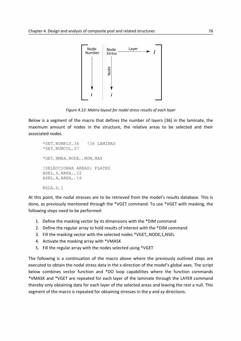
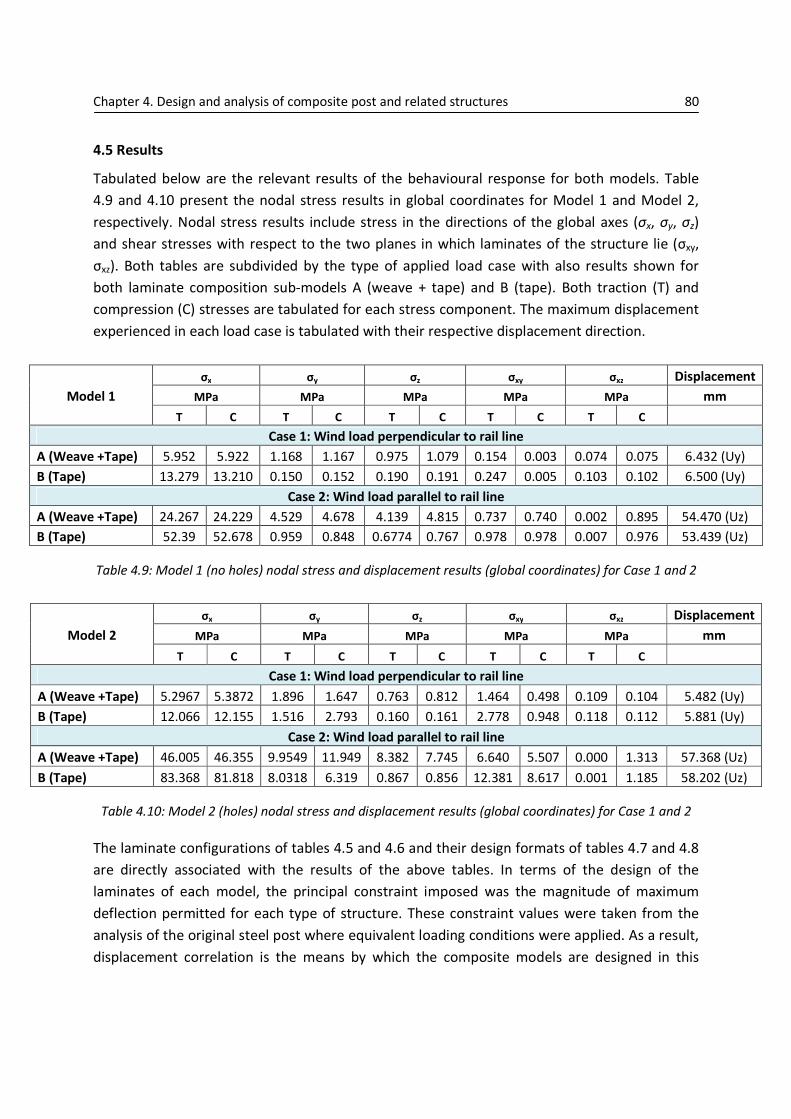
Tabulated below are the relevant results of the behavioural response for both models. Table
4.9 and 4.10 present the nodal stress results in global coordinates for Model 1 and Model 2,
respectively. Nodal stress results include stress in the directions of the global axes (σx, σy, σz)
and shear stresses with respect to the two planes in which laminates of the structure lie (σxy,
σxz). Both tables are subdivided by the type of applied load case with also results shown for
both laminate composition sub-models A (weave + tape) and B (tape). Both traction (T) and
compression (C) stresses are tabulated for each stress component. The maximum displacement
experienced in each load case is tabulated with their respective displacement direction.
σx σy σz σxy σxz Displacement
Model 1 MPa MPa MPa MPa MPa mm
T C T C T C T C T C
Case 1: Wind load perpendicular to rail line
A (Weave +Tape) 5.952 5.922 1.168 1.167 0.975 1.079 0.154 0.003 0.074 0.075 6.432 (Uy)
B (Tape) 13.279 13.210 0.150 0.152 0.190 0.191 0.247 0.005 0.103 0.102 6.500 (Uy)
Case 2: Wind load parallel to rail line
A (Weave +Tape) 24.267 24.229 4.529 4.678 4.139 4.815 0.737 0.740 0.002 0.895 54.470 (Uz)
B (Tape) 52.39 52.678 0.959 0.848 0.6774 0.767 0.978 0.978 0.007 0.976 53.439 (Uz)
Table 4.9: Model 1 (no holes) nodal stress and displacement results (global coordinates) for Case 1 and 2
σx σy σz σxy σxz Displacement
Model 2 MPa MPa MPa MPa MPa mm
T C T C T C T C T C
Case 1: Wind load perpendicular to rail line
A (Weave +Tape) 5.2967 5.3872 1.896 1.647 0.763 0.812 1.464 0.498 0.109 0.104 5.482 (Uy)
B (Tape) 12.066 12.155 1.516 2.793 0.160 0.161 2.778 0.948 0.118 0.112 5.881 (Uy)
Case 2: Wind load parallel to rail line
A (Weave +Tape) 46.005 46.355 9.9549 11.949 8.382 7.745 6.640 5.507 0.000 1.313 57.368 (Uz)
B (Tape) 83.368 81.818 8.0318 6.319 0.867 0.856 12.381 8.617 0.001 1.185 58.202 (Uz)
Table 4.10: Model 2 (holes) nodal stress and displacement results (global coordinates) for Case 1 and 2
The laminate configurations of tables 4.5 and 4.6 and their design formats of tables 4.7 and 4.8
are directly associated with the results of the above tables. In terms of the design of the
laminates of each model, the principal constraint imposed was the magnitude of maximum
deflection permitted for each type of structure. These constraint values were taken from the
analysis of the original steel post where equivalent loading conditions were applied. As a result,
displacement correlation is the means by which the composite models are designed in this
Chapter 4. Design and analysis of composite post and related structures 81
project. The displacements shown in the above table of results confirm this type of correlation.
Values of displacement for the set of sub-models A and B, in their respective case types, are
approximately equal with the largest variation between a sub-model set being just over 1 mm.
However, while the displacements of sub-model sets are equal, differences emerge in terms of
their maximum stresses experienced. With regards to the stress maximums along the direction
of the beam caused by bending (σx), each sub-model set demonstrate differences in magnitude
of approximately 100% between the A and B laminate types. Such variations in magnitude are
caused by variations in
1. Laminate stiffness
2. Sectional inertia
Laminate sub-model A for each case is composed of plies of woven and unidirectional fibres
whereas sub-model B is entirely compose of plies of unidirectional fibres. The differences in the
elastic constants of both types of plies can be appreciated by recalling table 3. It must be noted
that the elastic modulus is not the same as stiffness. It is instead a property of the constituent
material whereas stiffness is a property of the laminate structure. That is to say, the modulus is
an intensive property of the material whereas stiffness is an extensive property which is
dependent on the material, ply orientation, shape and boundary conditions of the structure. As
a consequence, the higher stiffness of the laminate B in the direction of the beam length
induces an increased load transfer and higher stress magnitude than that of the mixed ply
laminate of A. In order to maintain a comparable maximum displacement magnitude in the
lower stiffness laminate A to that of B, two approaches need to be performed: the first is by
adding additional woven plies to the laminate thereby increasing the inertia of the section to a
certain extent and the second is orientating unidirectional fibres along the direction of the
beam’s length.
Figures 4.14 and 4.15 show the stress variation in the x-direction σx around post section of
Model 1 for load Case 1 and load Case 2, respectively. Results for both sub-models A and B are
together for each load case. The section shown is equal to the section 40 mm above the fixed
end of the beam. Figure 4.13 depicts a sketch of the equivalent section with the dimensional
path related to the graphical figures defined also.

Chapter 4. Design and analysis of composite post and related structures 82
Figure 4.13: Beam section dimension for stress variation path
The figure below represents the loading perpendicular to the rail line in which stress maximums
in the x-direction are experienced over the thickness segments of the post structure with one
side in a state of tension and the opposing side of equal magnitude in compression. Between
these, the stress varies approximately linearly along the width of the structure with stresses
equal to zero occurring for both laminate A and B at the centre of the post’s width.
Figure 4.14: Stress Variation in post section at 40 mm above constraint boundary conditions
(Case 1)
0 200 400 600 800 1000-15
-10
-5
0
5
10
15
Length (mm)
Str
ess
(MP
a)
Stress Variation in Post Section for Case 1
1A:Weave & Tape
1B: Tape
Chapter 4. Design and analysis of composite post and related structures 83
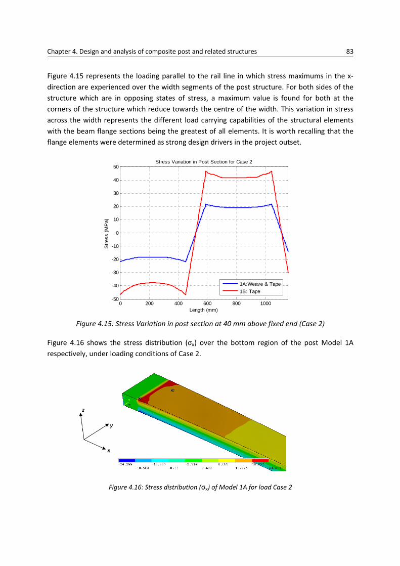
Figure 4.15 represents the loading parallel to the rail line in which stress maximums in the x-
direction are experienced over the width segments of the post structure. For both sides of the
structure which are in opposing states of stress, a maximum value is found for both at the
corners of the structure which reduce towards the centre of the width. This variation in stress
across the width represents the different load carrying capabilities of the structural elements
with the beam flange sections being the greatest of all elements. It is worth recalling that the
flange elements were determined as strong design drivers in the project outset.
Figure 4.15: Stress Variation in post section at 40 mm above fixed end (Case 2)
Figure 4.16 shows the stress distribution (σx) over the bottom region of the post Model 1A
respectively, under loading conditions of Case 2.
Figure 4.16: Stress distribution (σx) of Model 1A for load Case 2
0 200 400 600 800 1000-50
-40
-30
-20
-10
0
10
20
30
40
50
Length (mm)
Str
ess
(MP
a)
Stress Variation in Post Section for Case 2
1A:Weave & Tape
1B: Tape

Chapter 4. Design and analysis of composite post and related structures 84
Large variations are presented between the maximum stresses between Model 1 and Model 2
for load Case 2. The cause for such differences is the presence of holes in the plate elements of
the structure. These cut-outs provoke a stress concentration factor at the edge of the laminate.
As describe in Section 2, the stress concentration is caused by the combination of the fibre
direction and the load direction in which the material is subjected. The complexity of stress
analysis around the hole’s edge increases with the introduction of additional plies in the
laminate with various orientations. The stress concentrations occurring in such regions are
areas of concern and are therefore analysed using various strength criteria for failure analysis
as outlined previously in Section 4.3. Figure 4.18 shows the variation of nodal stress in the x-
direction around the hole edge for laminate sub-models A and B. The sketch in figure 4.17
depicts where the starting point and direction of the graphical stress distribution in figure 4.18.
Figure 4.17: Sketch of circumferential path for stress variation around hole
Figure 4.18: Stress variation in laminate around bottom hole for Model 2A and 2B, load case 2
0 100 200 300 400 500 600 700 800
0
10
20
30
40
50
60
70
80
90
Circumference (mm)
Str
ess
(MP
a)
Stress (sigmax) Distribution Around Bottom Plate Hole
2A) Weave + Tape
2B) Tape

Chapter 4. Design and analysis of composite post and related structures 85
Figure 4.19 shows the stress distribution (σx) over the bottom region of the post Model 2A
respectively, under loading conditions of Case 2.
Figure 4.19: Stress distribution (σx) of Model 2A for load Case 2
Tables 4.11 to 4.16 present the failure criteria results for both the predefined ANSYS failure
criteria and for the APDL macro failure criteria. Criteria include Tsai-Wu and Maximum Stress
for the predefined FEM program, and Tsai-Wu, Maximum Stress and Puck for the macro. Only
the most critical failure criteria results of the two models are presented below so as to reduce
the quantity of result information displayed. These critical failure values occur in Model 2
where the cut-outs/holes in the plate components creates stress concentrations in the laminate
bordering these regions as can be seen in the stress distribution of figure 4.17.
The failure criteria results are presented as failure index values where a value of one or above
signifies failure in one of the laminate’s layers. Both sets of results are obtained from nodal
stress data of each layer. Regions of high stress concentrations are analysed through one of the
defined failure criteria firstly by the APDL macro and secondly, by the predefined criteria in
ANSYS. By initially carrying out the failure analysis by the criteria written in the macro,
additional information such as the failure mode type and particular layer of failure are
attainable. The equivalent criterion analysis is then carried out in the ANSYS program in which
the user can define the desired layer for analysis, i.e. the layer at which failure has occurred in
the macro analysis. Failure index values and their node location are obtained and compared to
those of the macro.
Table 4.11 and 4.12 both present the most critical failure index values for the Tsai-Wu and
Maximum Stress, respectively, for laminate sub-model A analysed by both the ANSYS program
and the macro, with their % difference calculated and presented in the final column. Also
included are the node and layer number at which the critical index value occurs. Additional

Chapter 4. Design and analysis of composite post and related structures 86
information can be obtained from the APDL macro for the Maximum Stress criterion that
includes the mode in which the critical index value occurs. Table 4.13 presents the failure
analysis results for the Puck criterion defined in the APDL macro. Information including critical
node and layer number are obtained from the analysis. The macro also outputs the failure type
(FF or IFF) and in the case of the IFF, its mode number (1, 2, 3) for the most critical index value.
Tsai-Wu: Model 2A ANSYS Macro (APDL) % Difference
FPF Index Value 0.13800 0.13816 0.1%
Node 15322 15322
Layer 34 34
Table 4.11: Tsai-Wu Index failures for Model 2A in FEM (ANSYS) and macro program (APDL)
Max Stress: Model 2A ANSYS Macro (APDL) % Difference
FPF Index Value 0.12216 0.12223 (Yt) 0.05%
Node 15322 15322
Layer 34 34
Table 4.12: Maximum Stress Index failures for Model 2A in FEM (ANSYS) and macro program (APDL)
Puck: Model 2A Macro (APDL)
FPF Index Value 0.12303
Failure Mode 1 (IFF)
Node 15322
Layer 34
Table 4.13: Puck Index failure for Model 2A in macro program (APDL)
Tables 4.14 to 4.15 below present the equivalent result format as for the set of tables above,
however this time the results presented are for the model composed of laminate sub-model B.
Again, the Tsai-Wu and Maximum Stress criteria are given in the first two tables for both the
ANSYS and APDL analysis. The third table contains the results of the Puck criterion for the APDL
analysis only.
Tsai-Wu: Model 2B ANSYS Macro (APDL) % Difference
FPF Index Value 0.11787 0.11770 0.14%
Node 12728 12728
Layer 1 1
Table 4.14: Tsai-Wu Index failures for Model 2B in FEM (ANSYS) and macro program (APDL)

Chapter 4. Design and analysis of composite post and related structures 87
Max Stress: Model 2B ANSYS Macro (APDL) % Difference
FPF Index Value 0.10917 0.10902 0.13%
Node 12728 12728
Layer 1 1
Table 4.15: Maximum Stress Index failures for Model 2B in FEM (ANSYS) and macro program (APDL)
Puck: Model 2B Macro (APDL)
FPF Index Value 0.10902
Mode FF
Node 12728
Layer 1
Table 4.16: Puck Index failure for Model 1B in macro program (APDL)
All of the above criteria results demonstrate that failure does not occur in any of the structures
(i.e. index failure < 1). However, it is worth noting that the more critical index failures occur for
the sub-model A (weave + tape) even though the stress concentrations around the holes shown
in figure 4.19 are greater in sub-model B (tape).
The index result values for the predefined ANSYS criteria and APDL macro criteria are identical
for each criterion with only minute differences between the results occurring due to variation
of precisions.

Chapter 4. Design and analysis of composite post and related structures 88
4.6 Validation of Numerical Model
Two procedures have been implemented to verify the adequacy of the FEM model. These
include
1. Classical Lamination Theory (CLT) for Narrow Beams [15], [16], [17]
2. Smeared Approach
Both procedure types compare stress results for a given section of the post with those obtained
in the FEM model. The accuracy of both the CLT and Smeared Approach validation methods are
analysed in terms of their axial stiffness, curvature and bending stiffness results with the
effectiveness and restrictions of each of the procedures considered.
4.6.1 Classical Lamination Theory for Narrow Beam
The response of the beam is dependent on the width to height ratio of the beam’s section. A
beam of a small ratio is defined as being ‘narrow’ while that of a large section ratio is defined as
a ‘wide’ beam. The difference in response for both beam types is related to the significance of
the induced lateral curvature caused by the beam subjected to axial bending. For the narrow
beam the axial strain distribution gives rise to a significant amount of deformation of the cross-
section which is induced due to the Poisson effect. Figure 4.20 shows a simplified
representation of the response of a narrow beam. As a result, loading Nx and moment Mx acting
on the axial directions are considered while lateral moment is concluded as being equal to zero.
In summary, the initial conditions of a narrow beam,
0==== xyyxyy MMNN
0≠yK (4.17)
Figure 4.20: Narrow composite beam deformed cross-section

Chapter 4. Design and analysis of composite post and related structures
The Classical Laminate Theory (CLT) of Chapter Two is applied
validity of the numeric model of the FEM.
stiffness, bending stiffness and stres
figure 4.21. The process includes the CLT described in Chapter Two up to determination of the
extension, coupling and bending stiffness. From that point, the narrow beam conditions are
implemented and the responses are subsequently determined in the order shown in the
flowchart. The CLT validation is written using MATLAB parametric language.
Figure 4.21: Classical Laminate Theory
The theory described below relates t
of the flowchart in figure 4.21.
load-deformation relation can be summarized as
or as its inverse
Material Data + Structural
Configuration
Axial Stiffness (EA) Bending Stiffness (EI)
Centroid (ZC)
of composite post and related structures
The Classical Laminate Theory (CLT) of Chapter Two is applied in this section
validity of the numeric model of the FEM. Comparable response results such as the axial
stiffness, bending stiffness and stresses are calculated using the process shown as a flowchart in
figure 4.21. The process includes the CLT described in Chapter Two up to determination of the
extension, coupling and bending stiffness. From that point, the narrow beam conditions are
d and the responses are subsequently determined in the order shown in the
flowchart. The CLT validation is written using MATLAB parametric language.
: Classical Laminate Theory (CLT) process for narrow beam
The theory described below relates to the Narrow Beam Theory step and the subsequent steps
of the flowchart in figure 4.21. Recalling the constitutive equations in (2.50) and (2.51), the
can be summarized as
=
kDB
BA
M
N oε.
=
M
N
db
ba
k T
o
.ε
Compliance Matrix [S]
Reduced Stiffness [Q]
Narrow Beam Theory
Inverse Compliance
Matrix
NX, MX, MXY
εX, εY, εXY
kX, kY, kXY
σ = Q.ε
89
in this section to verify the
Comparable response results such as the axial
ses are calculated using the process shown as a flowchart in
figure 4.21. The process includes the CLT described in Chapter Two up to determination of the
extension, coupling and bending stiffness. From that point, the narrow beam conditions are
d and the responses are subsequently determined in the order shown in the
flowchart. The CLT validation is written using MATLAB parametric language.
(CLT) process for narrow beam
o the Narrow Beam Theory step and the subsequent steps
Recalling the constitutive equations in (2.50) and (2.51), the
(4.18)
(4.19)
Transformed Stiffness [Q]
Extension [A] Coupling [B] Bending [D]

Chapter 4. Design and analysis of composite post and related structures 90
Applying the initial conditions of the narrow beam, where Ny= Nxy= My= Mxy = 0, the relation is
reduced to the following equations
xxox MbNa 1111 +=ε
xxx MdNbk 1111 +=
(4.20)
or its matrix form as
=
x
x
x
ox
M
N
db
ba
k.
1111
1111ε
(4.21)
And inverting back the matrix as the load-deformation relation
=
−
x
ox
x
x
kdb
ba
M
N ε.
1
1111
1111 =>
=
x
ox
x
x
kDB
BA
M
N ε.
'
''
11
11
(4.22)
where
11
211
11
1
1'
d
ba
A−
=
(4.23)
11
111111
1
1'
b
dab
B−
=
(4.24)
11
211
11
1
1'
a
bd
D−
=
(4.25)
The load-deformation relation of equation (4.22) for the plate and flange laminates in the xy-
plane (i = 1, 2, 3, 4) can be expressed by the following two equations.
ixio
ixiix kBAN ,,1,,1, '' += ε
ixio
ixiix kDBM ,,1,,1, '' += ε
(4.26)
However, for the web laminate in the xz plane (i = 5), no radius of curvature exists.
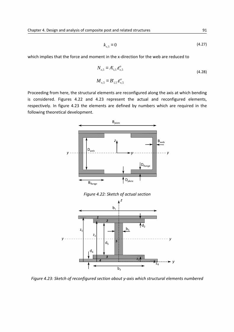
Chapter 4. Design and analysis of composite post and related structures 91
05, =xk (4.27)
which implies that the force and moment in the x-direction for the web are reduced to
oxx AN 5,5,15, ' ε=
oxx BM 5,5,15, ' ε=
(4.28)
Proceeding from here, the structural elements are reconfigured along the axis at which bending
is considered. Figures 4.22 and 4.23 represent the actual and reconfigured elements,
respectively. In figure 4.23 the elements are defined by numbers which are required in the
following theoretical development.
Figure 4.22: Sketch of actual section
Figure 4.23: Sketch of reconfigured section about y-axis which structural elements numbered
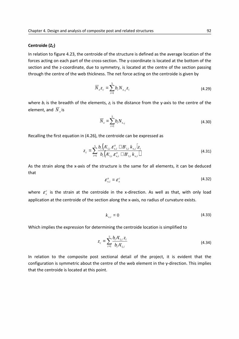
Chapter 4. Design and analysis of composite post and related structures 92
Centroide (ZC)
In relation to figure 4.23, the centroide of the structure is defined as the average location of the
forces acting on each part of the cross-section. The y-coordinate is located at the bottom of the
section and the z-coordinate, due to symmetry, is located at the centre of the section passing
through the centre of the web thickness. The net force acting on the centroide is given by
∑=
=5
1,
iiixicx zNbzN (4.29)
where bi is the breadth of the elements, zi is the distance from the y-axis to the centre of the
element, and xN is
∑=
=5
1,
iixix NbN (4.30)
Recalling the first equation in (4.26), the centroide can be expressed as
( )( )∑
= ++
=5
1 ,,1,,1
,,1,,1
''
''
i ixio
ixii
iixio
ixiic kBAb
zkBAbz
εε
(4.31)
As the strain along the x-axis of the structure is the same for all elements, it can be deduced
that cx
oix εε =, (4.32)
where cxε is the strain at the centroide in the x-direction. As well as that, with only load
application at the centroide of the section along the x-axis, no radius of curvature exists.
0, =ixk (4.33)
Which implies the expression for determining the centroide location is simplified to
∑=
=5
1 ,1
,1
'
'
i ii
iiic Ab
zAbz
(4.34)
In relation to the composite post sectional detail of the project, it is evident that the
configuration is symmetric about the centre of the web element in the y-direction. This implies
that the centroide is located at this point.

Chapter 4. Design and analysis of composite post and related structures 93
Axial Stiffness (EA)
In relation to calculating the axial stiffness, an axial force is applied at the centroide of the
entire section. The entire force in the x-direction can be written as
cxx AEN ε= (4.35)
where AE is the equivalent axial stiffness of the entire section. Substituting the equations
(4.26) and (4.28) into (4.30), the total force is
( ) ( )ox
iixi
oixiix AbkBAbN 5,5,15
4
1,,1,,1 ''' εε +
+= ∑=
(4.36)
and recalling the conditions of the axial force in (4.32) and (4.33), the total force can be written
as
( ) cx
iiix AbN ε
= ∑
=
5
1,1' (4.37)
where the total axial stiffness is
( )ii
i AbAE ,1
5
1
'∑=
=
(4.38)
Bending Stiffness (EI)
The axial bending stiffness can be determined by a moment applied at the centroide which is
equal to the bending stiffness multiplied by the curvature experienced at the centroide and is
given in the following expression.
cx
cxx kDM = (4.39)
The total moment is made up of moment and force components, in the x-direction, of the five
sectional elements.
( ) 5,
4
1,,, x
iiixiixiix MzNbMbMC
++=∑=
(4.40)
where the moment at the web (i = 5) is
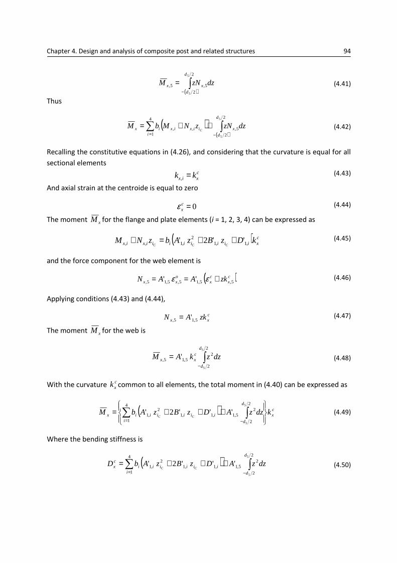
Chapter 4. Design and analysis of composite post and related structures 94
( )∫
−
=2
2
5,5,
5
5
d
d
xx dzzNM
(4.41)
Thus
( )( )∫∑
−=
++=2
2
5,
4
1,,
5
5
d
d
xi
iixixix dzzNzNMbMC
(4.42)
Recalling the constitutive equations in (4.26), and considering that the curvature is equal for all
sectional elements
cxix kk =, (4.43)
And axial strain at the centroide is equal to zero
0=cxε (4.44)
The moment xM for the flange and plate elements (i = 1, 2, 3, 4) can be expressed as
( ) cxiiiiiiiixix kDzBzAbzNM
CCC ,1,12
,1,, ''2' ++=+ (4.45)
and the force component for the web element is
( )cx
cx
oxx zkAAN 5,5,15,5,15, '' +== εε (4.46)
Applying conditions (4.43) and (4.44),
cxx zkAN 5,15, '= (4.47)
The moment xM for the web is
dzzkAMd
d
cxx ∫
−
=2
2
25,15,
5
5
'
(4.48)
With the curvature cxk common to all elements, the total moment in (4.40) can be expressed as
( ) cx
d
diiiiiiix kdzzADzBzAbM
CC
+++= ∫∑−=
2
2
25,1
4
1,1,1
2,1
5
5
'''2'
(4.49)
Where the bending stiffness is
( ) dzzADzBzAbDd
diiiiiii
cx CC ∫∑
−=
+++=2
2
25,1
4
1,1,1
2,1
5
5
'''2'
(4.50)

Chapter 4. Design and analysis of composite post and related structures 95
Knowing the bending stiffness and total moment, the curvature can be found by manipulating
the above equation into the form below.
cx
xcx
D
Mk =
(4.51)
The stresses and strains are calculated using equations in (2.44) and (2.45) of Chapter Two, and
are recalled as
+
=
ixy
iy
ix
ik
oixy
oiy
oix
kixy
iy
ix
k
k
k
z
,
,
,
,
,
,
,
,
,
,
γ
ε
ε
ε
ε
ε
(4.52)
[ ] [ ] [ ]kikki Q εσ = (4.53)
The relation of the laminate force and moments to strains and curvatures, which is expressed in
the equations of (4.26), is used to determine the force and moments at a specific laminate. The
bending stiffness conditions of (4.43) and (4.44) are implemented in the equations of (4.26).
The strains and curvatures are calculated by the inverse constitute relation in (4.19). The
transformed stiffness ijQ is calculated for each layer of the laminate and subsequently
multiplied by the strain of the corresponding layer. Note that the curvature component of the
strain in (4.52) is dependent on the distance of the particular layer of interest from the
centroide (zk). This process is carried out for each laminate element in the section. Using the
bending stiffness approach, the steps in determining the stresses and strains are summarised as
follows.
1. Calculate the bending stiffnesscxD
2. Knowing the moment xM , calculate the curvature cxk from equation (4.51)
3. Applying bending stiffness conditions in (4.43) and (4.44), find the force Nx and
moments Mx and Mxy using equations in (4.26)
4. Determine strains and curvatures from the deformation-load relation in (4.19)
5. Multiply the transformed stiffness matrix ijQ of a particular layer by its corresponding
strains and curvatures to determine the stresses in that layer.

Chapter 4. Design and analysis of composite post and related structures 96
4.6.2 The Smeared Approach
The smeared approach involves determining the equivalent axial Elastic Modulus Ex for the
composite section. This approach is based on the assumption that the equivalent Elastic
Modulus is constant throughout the laminate. While it is a more simplistic method of
determining responses, it does not consider the effect of the stacking sequence of the laminate.
Knowing the elastic constants values in principal directions (1, 2) and orientation of the fibres
for a given layer, the equivalent axial Elastic Modulus Ex for off-axis fibres can be determined
from the relation of the transformed compliances ijS in (2.32).
ki
ki
ki
ki
x EEGEEθθθνθ 4
22
22
11
12
12
4
11
sin1
sincos21
cos11 +
−+= (4.54)
where i is the laminate element (plate, flange, or web) and k is the particular layer in the
laminate. The equivalent axial Elastic Modulus is calculated by multiplying the transformed
stiffness in (4.54) in each layer by its corresponding layer thickness and dividing by the overall
thickness of the laminate.
∑=
=5
1
,,
iki
ki
kix
ixt
tEE (4.55)
The total equivalent axial stiffness is gotten by summing the equivalent stiffness of each
element (i = 1, 2, 3, 4, 5).
∑=
=5
1,
iiix AEAE (4.56)
where Ai is the sectional area. Similarly, the bending stiffness is calculated by summing the
individual sectional elements.
∑=
=5
1,
iiix IEIE (4.57)
As this approach is based on the assumption that the equivalent Elastic Modulus is constant
throughout the laminate, the centroide zi is always located at the mid-plane of each laminate.
The centroide of the entire section is found by the summation of all the laminate stiffnesses
multiplied by their corresponding centroide, and dividing them by the total stiffness equivalent.
( )∑
=
=5
1 ,
,
i iix
iiixc AE
zAEz (4.58)

Chapter 4. Design and analysis of composite post and related structures 97
At this point, the maximum stresses for a given point in the section are determined. To
incorporate the variation of equivalent stiffness between the sectional elements, the equivalent
width technique is used. From equation (4.55), the equivalent axial Elastic Modulus for the
plate element (sections 1 and 4) is determined to be the stiffer than the beam elements
(sections 2, 3, and 5). That implies that to maintain an equivalent stiffness throughout the
entire section, the geometric sectional properties of the plate elements must be altered by a
factor of n where
beam
plate
E
En = (4.59)
Consider the two sectional drawings in figures 4.23 and 4.24, the first figure shows the original
section with elements of varying stiffness (Ex,plate, Ex,beam) whereas the second figure depicts the
equivalent section in which all elements have the same stiffness value (Ex,beam) and also shows
the necessary geometric transformation to maintain the mechanical properties of the original
section. Note that due to symmetry, the section elements below the plane y-y are considered
to take on the same transformation of their symmetric counterparts above. This also implies
that the centroide zc remains at the centre of the entire section.
Figure 4.24: Original section configuration, elements of varying stiffness

Chapter 4. Design and analysis of composite post and related structures 98
Figure 4.25: Transformed section configuration, elements of equivalent stiffness
The inertia Iyy of the entire section is recalculated, implementing this time the transformation in
figure 4.24. The stress at the plate extremity is calculated using the beam bending relationship
multiplied by the transformation factor n.
=
I
yMn i
i
.σ (4.60)
4.6.3 Results Comparison
One composite model type is used for the results comparison. The model type chosen is the
composite structure without holes and laminates of unidirectional fibres only, i.e. Model 1B. As
the structure is of variable section along its length, the section dimensions above the fixed end
are chosen. This is equivalent to the section at 200 mm above the bottom of the post. The
loading is of Load Case 2, i.e. wind loading parallel to the rail line which has an equivalent total
moment M of 17790 Nm about the y-axis.
Table 4.17 presents the results for the both the CLT and Smeared Approach validation models.
The results include the centroide location, axial stiffness, curvature, and bending stiffness. A
percentage difference between the two sets of results is made also. Note that the FEM results
are not included in this table as the structure’s variable section along its length affects the axial
stiffness, curvature, and bending results.

Chapter 4. Design and analysis of composite post and related structures 99
Units CLT for Narrow
Beams
Smeared
Approach
% Difference
Centroide (zc) mm 70 70 0.0%
Axial Stiffness (EA)x N 8.3999e8 8.8244e8 5.1%
Curvature (kc)x mm
-1 5.7853e-6 5.3755e-6 7.1%
Bending Stiffness (EI)x Nmm2
3.0578e12 3.2908e12 7.6%
Table 4.17: Behavioural response result comparison for CLT for narrow beams and the smeared approach
As both the entire structural section and each laminate element are symmetric about the y-
plane, the centroide distances are the same for both the CLT and Smeared Approach analyses.
Variation between both validation models occurs for the axial stiffness, curvature and bending
stiffness. This occurs due to the presence of extension, coupling and bending parameters (A’i,
B’i, D’j) in the CLT model while the Smeared Approach is an analogous method of elastic
equivalents (Ex) and sectional properties (area and moment inertia) used to determine intrinsic
laminate response. As all the laminates are symmetric about one plane (y-plane) they can be
classified as monoclinic, which causes the coupling terms B’I to be reduced to zero meaning that
only extension and bending terms remain. The difference between the two models increases if
the ply stacking sequence is altered to an un-symmetric configuration where coupling returns
to the load-deformation relation.
The maximum stresses of the plate element in a state of tension are tabulated below in table
4.18. They include results for the FEM, CLT, and Smeared Approach. Both the FEM and CLT
results are presented at a layer level while the Smeared Approach stress result is of a laminate
level. Both the FEM and CLT results are the maximum tensile stresses experienced and occur in
the top layer (0o) of the top laminate, i.e. the layer furthest from the centroide of the section.
The higher stiffness caused by the ply orientation and its distance from the centroide confirms
that maximum stresses would develop in this zone of the cross-section. The minute difference
between both results (1.24%) would indicate that the approximation made in the FEM model of
the composite post is valid. The large variation between the Smeared Approach and FEM/CLT
models indicates the limitations incurred by assuming equivalent elastic properties for a
laminate as opposed to a layer analysis made in the CLT for Narrow Beams. The Smeared
Approach does not account the for the stress variations between layers and consequently
underestimates the maximum stress incurred in the section.
Location σx (N/mm2)
FEM Top Plate (1) 0o Ply 52.390
CLT for Narrow Beams Top Plate (1) 0o Ply 53.046
Smeared Approach Top Plate (Laminate) 38.637
Table 4.18: Stress result comparison for FEM, CLT for narrow beams, and the smeared approach

Chapter 4. Design and analysis of composite post and related structures 100
4.7 Analysis Under Other Various Loading Types
The primary objective of the design-analysis for the proposed post is to ensure behavioural
response compliance between it and the original post, i.e. both the original and proposed post
have similar maximum deflections and factor of safety magnitudes for stresses (σmax/ σult). This
objective was undertaken using equivalent loading conditions for both structures. After
determining an adequate design for the proposed structure, a subsequent or secondary load
analysis can be considered. This secondary load analysis composes of
1. Dynamic loading
2. Loading hypothesis
Both of these additional types of loading account for conditions that are experienced by the
post structure at instantaneous, temporary, and permanent levels. The loading types are
caused by the post’s proximity to moving trains (dynamic loading), by related structural
components joined to the post (load hypothesis) and additional loading related to seasonal
changes (loading hypothesis).
4.7.1 Dynamic Loading
4.7.1.1 Background and Development
It is well known that relatively-high to high velocity trains can exert aerodynamic loading on
objects in their proximity. An isolated train passing through the air induces a complicated flow
field that are best simulated in computational fluid mechanics (CDF) simulations and finite
volume numerical methods. However, in order to simulate a typical aerodynamic pressure
exerted on the post structure a number of papers related to this phenomenon [18], [19], [20]
were analysed and an appropriate pressure loading consistent with the conditions of the
project was applied dynamically in ANSYS.
The overall resistance R to movement (on level track) that needs to be overcome by the
traction effort of the locomotive is a result of rolling friction between wheel and rail, bearing
resistance, train dynamic loses and air resistance, and are presented in the following empirical
expression.
A
A
S
Ypp
CC 122 = (4.61)
where A and B.V are the mechanical resistances and C.V2 is the aerodynamic resistance. By
specifically analysing this external aerodynamic resistance part of the expression, it can be
further expressed in terms of the coefficient C:
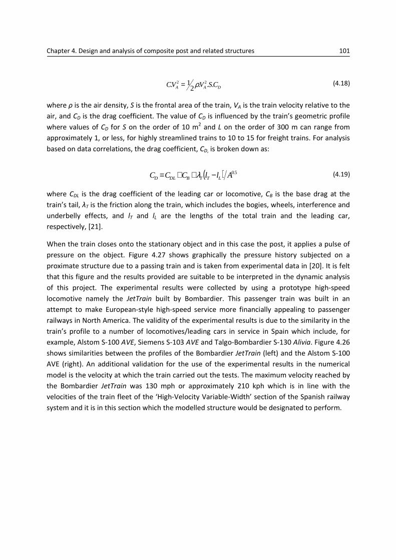
Chapter 4. Design and analysis of composite post and related structures 101
DAA CSVVC ...21. 22 ρ=
(4.18)
where ρ is the air density, S is the frontal area of the train, VA is the train velocity relative to the
air, and CD is the drag coefficient. The value of CD is influenced by the train’s geometric profile
where values of CD for S on the order of 10 m2 and L on the order of 300 m can range from
approximately 1, or less, for highly streamlined trains to 10 to 15 for freight trains. For analysis
based on data correlations, the drag coefficient, CD, is broken down as:
( ) 5.0AllCCC LTTBDLD −++= λ
(4.19)
where CDL is the drag coefficient of the leading car or locomotive, CB is the base drag at the
train’s tail, λT is the friction along the train, which includes the bogies, wheels, interference and
underbelly effects, and lT and lL are the lengths of the total train and the leading car,
respectively, [21].
When the train closes onto the stationary object and in this case the post, it applies a pulse of
pressure on the object. Figure 4.27 shows graphically the pressure history subjected on a
proximate structure due to a passing train and is taken from experimental data in [20]. It is felt
that this figure and the results provided are suitable to be interpreted in the dynamic analysis
of this project. The experimental results were collected by using a prototype high-speed
locomotive namely the JetTrain built by Bombardier. This passenger train was built in an
attempt to make European-style high-speed service more financially appealing to passenger
railways in North America. The validity of the experimental results is due to the similarity in the
train’s profile to a number of locomotives/leading cars in service in Spain which include, for
example, Alstom S-100 AVE, Siemens S-103 AVE and Talgo-Bombardier S-130 Alivia. Figure 4.26
shows similarities between the profiles of the Bombardier JetTrain (left) and the Alstom S-100
AVE (right). An additional validation for the use of the experimental results in the numerical
model is the velocity at which the train carried out the tests. The maximum velocity reached by
the Bombardier JetTrain was 130 mph or approximately 210 kph which is in line with the
velocities of the train fleet of the ‘High-Velocity Variable-Width’ section of the Spanish railway
system and it is in this section which the modelled structure would be designated to perform.

Chapter 4. Design and analysis of composite post and related structures 102
Figure 4.26: Bombardier JetTrain and Alstom S-100 AVE
In relation to the graph in figure 4.27, above the zero mark represents the positive pressure
exerted on an adjacent structure and below zero represents the negative pressure or vacuum
created. Maximum values on the graph range from approximately 0.06 psig to 0.09 psig or
413.68 Pa and 620.58 Pa, respectively. The concluding information gathered by the reports
allowed the author to make a more conservative representation of the pressure exerted on the
post as train velocities. It is worth highlighting that this proposed post would not be designated
for such rail High-Velocity only corridors, can reach up to 350 kph (Siemens S-103 AVE) but for
the general rail lines (via general) of reduce velocity capacities.
Aerodynamic pressures, which include a Factor of Safety of 2.0, utilised in the numerical
program include a maximum pressure value of 1.2 MPa at the point at which the nose of the
leading car reaches the structure and, in a relatively instantaneous moment, a pulse of vacuum
of 1.4 MPa which has the opposite directional loading effect and occurs when the nose of the
train immediately passes the structure. As a result, the numerical model intends to simulate an
equivalent pressure change applied on the structure. Figure 4.28 is a representation of the load
history inputted into the transient analysis of the numerical model. The pressure history below
also highlights an interesting phenomenon that consists of a number of relatively large pressure
variations contained within the passing of the nose and tail of the train. The figure shows two
pressure spikes sustained in the negative portion of the pressure curve. These variations are
directly related to the discontinuities of the train, i.e. the inter-car gaps of the passing train.
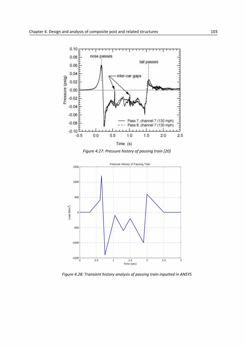
Chapter 4. Design and analysis of composite post and related structures 103
Figure 4.27: Pressure history of passing train [20]
Figure 4.28: Transient history analysis of passing train inputted in ANSYS
0 0.5 1 1.5 2 2.5 3-1500
-1000
-500
0
500
1000
1500
Time (sec)
Load
(N
/m2 )
Pressure History of Passing Train

Chapter 4. Design and analysis of composite post and related structures 104
4.7.1.2 Modal Analysis
Modal analysis is used to determine the vibration characteristics (natural frequencies and mode
shapes) of a structure. It also can be a starting point for another, more detailed, dynamic
analysis, such as a transient dynamic analysis, a harmonic response analysis, or a spectrum
analysis. Modal analysis uses the structure’s overall mass and stiffness to determine the various
periods that it will naturally resonate at. This issue is important in the design stage of the
structure as dynamic loading such as wind and aerodynamic pulse loading from passing trains
can cause the structure to vibrate and if this excitation coincides with the natural frequency of
the structure resonance will occur which can be detrimental to the structure’s performance.
Following the modal analysis, a transient analysis of the post structure is carried out. Tables
4.19 and 4.20 show the first three natural frequencies of the composite structure calculated in
ANSYS (ANTYPE, MODAL) and also below are the mode shapes of their natural frequencies for
Model 1A [8].
Mode 1A 1B
(Hz) (rad/s) (Hz) (rad/s)
1 6.335 39.805 8.768 55.089
2 19.617 123.257 15.355 96.478
3 158.415 995.349 176.572 1109.433
Table 4.19: Modal analysis, first three natural frequencies of post in Model 1
Mode 2A 2B
(Hz) (rad/s) (Hz) (rad/s)
1 4.249 26.694 5.151 32.364
2 12.941 81.311 15.375 96.607
3 45.721 287.272 64.859 407.522
Table 4.20: Modal analysis, first three natural frequencies of post in Model 2
Figure 4.29: Mode 1 shape for 1B

Chapter 4. Design and analysis of composite post and related structures 105
Figure 4.30: Mode 2 shape for 1B
Figure 4.31: Mode 3 shape for 1B
4.7.3 Transient Analysis
Transient dynamic analysis (sometimes called time-history analysis) is a technique used to
determine the dynamic response of a structure under the action of any general time-dependent
loads. The basic equation of motion solved by the transient analysis is:
[ ][ ] [ ][ ] [ ][ ] )(tFuKuCuM =++ &&&
(4.20)
where M is the mass matrix, C is the damping matrix, K is the stiffness matrix, u is the nodal
displacement vector, u& is the nodal velocity vector, and u&& is the nodal acceleration vector.
In this project, the transient analysis is used to determine the time-varying stresses and
displacements in the structure as it responds to a prescribed variable load history. The
experimental load-history curve shown in figure 4.27 is applied in the transient analysis in
ANSYS. Figure 4.28 shows the approximated, more conservative load history converted from
psig to N/m2. The transient analysis involves loads which are functions of time, and thus are
divided into load steps. For each load step, the load and time values are specified with the
option to specify whether the load is applied as a ramp function (KBC,0) or as a step function

Chapter 4. Design and analysis of composite post and related structures 106
(KBC,1). The time value is specified after the load is applied via the TIME command. The load-
history curve is solved by employing time integration of the equations of motion with the
integration time step (ITS) used as the time increment in this process. The size of time
increment step determines the accuracy of the transient solution where the smaller the
increment the more accurate the solution [22]. There are three methods of transient analysis
available which include Full, Reduced and Mode Superposition Method and are implemented
through the TRNOPT command. The one used in this analysis is the Full Method as it permits all
types of non-linearities however it is much more CPU intensive than the other two methods as
the full system matrices are used [23].
In most structures, damping is present in some form. The problem of dissipating the energy in
structures is an important feature in mechanical design in terms of vibration control, noise and
fatigue endurance. The amplitude and frequency of vibration in a structure is controlled by the
applied excitation and the response of the structure to that particular excitation. Damping
becomes important in the structure when the response is close to the natural/resonant
frequency or if the vibration response is short term. Energy dissipation mechanisms are
separated into classes: the first is damping in the structure due to friction at joints. While this
source is usually dominant in metal structures it does not contribute significantly to composite
structures as joints are tended to be kept to a minimum or are adhesively bonded. The second
class and more predominant of the two is inherent material damping [24]. For fibre reinforced
composite materials, material damping is dependent on two mechanism types: at a microscale
level, the energy dissipation is induced by viscoelastic behaviour of the matrix, damping at the
fibre-matrix interface, and damping due to damage. The second type is at the laminate level
where energy dissipation is dependent on the constituent properties, the ply orientation,
interlaminar effects, and stacking sequence [25].
In relation of the finite element model, damping is provided by Rayleigh damping equation
which is represented by the expression
KMC βα +=
(4.21)
where C is the damping matrix, M is the mass matrix and K is the stiffness matrix. The
parameters α and β are inputted into the program through the ALPHAD (mass damping) and
BETAD (material damping) commands, respectively. The parameters α and β are unknowns but
are related to the modal damping ratio ξ. The modal damping ratio is the ratio of actual
damping to the critical damping for a particular mode of vibration. If ωi is the natural frequency
(as calculated previously in the modal analysis) of mode i, then α and β satisfy the relation

Chapter 4. Design and analysis of composite post and related structures 107
22
i
ii
βωωαξ +=
(4.22)
Figure 4.32 below describes the influence of each of the parameters over a range of natural
frequencies. For damping of at low frequencies, α plays a more dominant role whereas higher
frequencies are damped more by the β parameter and to a lesser extent by α-damping.
Figure 4.32: Influence of α and β over a range of natural frequencies
To specify both α and β for a given damping ratio, it can be assumed that the sum of the two
damping functions is nearly constant over a range of frequencies. Therefore, given a modal
damping ratio ξ and a frequency range ωi and ωj, two simultaneous equations can be solved for
α and β [8].
22
i
i
βωωαξ +=
22j
j
βωωαξ +=
(4.23)
In relation to the transient analysis presented in the project, only one model type and material
configuration was analysed. This is predominantly due to the intensive computational demands
required to carry out a full transient analysis on models with a large quantity of elements such
is the case in this project. The structure without holes composed of only laminates with
unidirectional material (1B) was analysed. To specify both α and β for a given damping ratio,
the first two modal natural frequencies (ω1 and ω2) of the model were taken from table 4.19
and solved in the above simultaneous equations. The damping ratio ξ of carbon fibre
composites is known to approximately 0.01 [26]. The values yielded from the above
simultaneous equations include 0.7 and 0.00132 for the α-damping and β-damping,
respectively.

Chapter 4. Design and analysis of composite post and related structures 108
It must be stressed that the relevant data for damping of a particular composite laminate
structure requires a certain degree of vibration damping experiments at a laminate and possibly
a structural level. The above damping parameter values accumulated are approximations and
their response results obtained in the transient analysis are viewed with caution. A number of
additional transient analyses were carried out with varying α and β values so as to show the
influence of both types of damping on the structure. Figure 4.33 shows the vibration response
of Model 1B caused by the given excitation in figure 4.28 for different values of the α and β
parameters. Figure 4.34 shows the stress variation in the x-direction at the bottom of the
structure (node 4553), close to the fixed end of the beam caused by the same load history.
The behaviour responses of the figures below indicate the importance of dynamic response
analysis. The initial two loadings applied to the structure occur in opposite directions, which
simulates a positive-negative pressure condition caused by the passing train. This load pair
induces an initial displacement of 32.14 mm and a subsequent displacement in the opposite
direction of 79.2 mm from its stationary position. The range of displacement of the pair is equal
to 111.34 mm and occurs over a time interval of 0.11 s whereas the maximum displacement for
this model in the static analysis was 53.439 mm. Dynamic ranges of this magnitude over a large
number of cycles can merit the need for a fatigue analysis. As this structure is intended for only
temporary substitution of a fail post structure, its service life duration is relatively low and for
that reason a fatigue analysis is not considered.
In terms of the effect α and β damping values, the analysis demonstrates that both damping
parameters influence the overall damping of the structure. The vibration response below shows
that in the case of reduced α and β damping values, the damping is significantly less than that
of the two cases where alternately one of the damping values is reduced. In both these cases,
the damping response is quite similar.
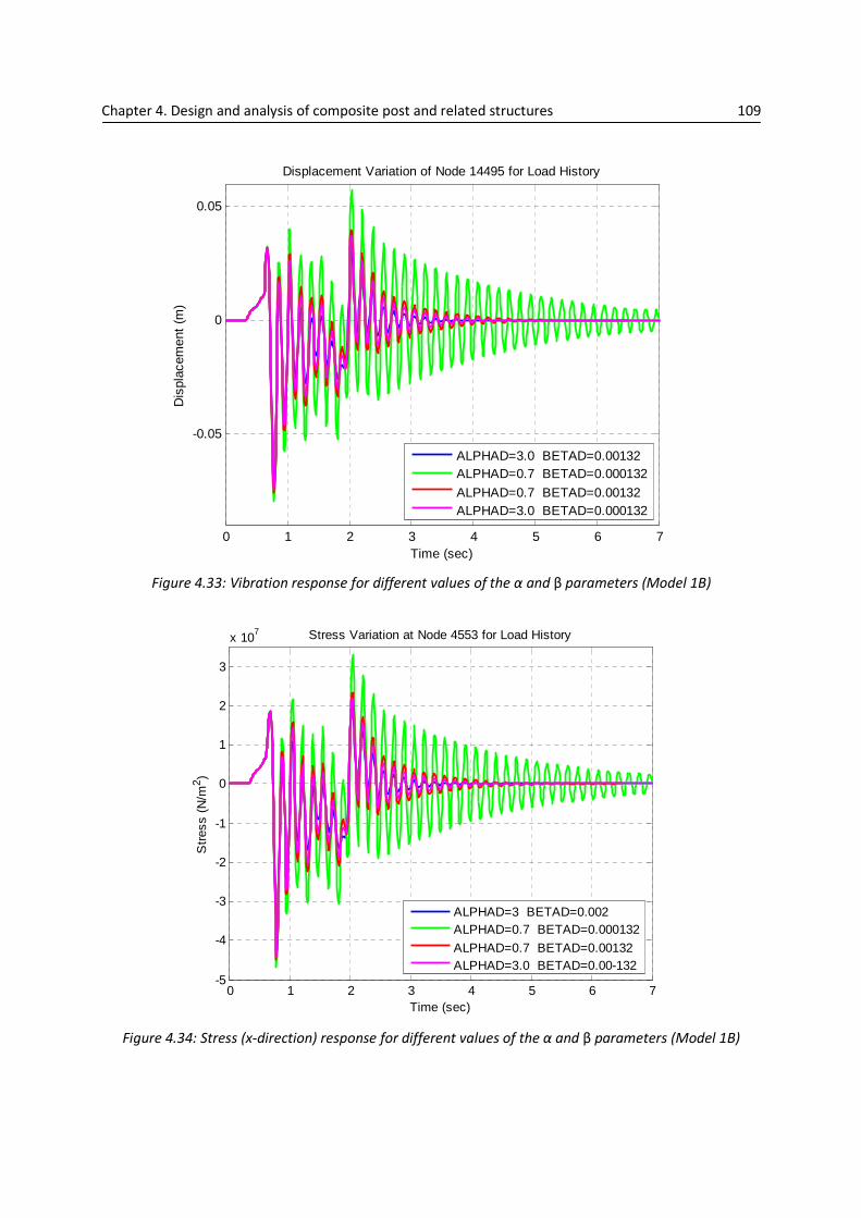
Chapter 4. Design and analysis of composite post and related structures 109
Figure 4.33: Vibration response for different values of the α and β parameters (Model 1B)
Figure 4.34: Stress (x-direction) response for different values of the α and β parameters (Model 1B)
0 1 2 3 4 5 6 7
-0.05
0
0.05
Time (sec)
Dis
plac
emen
t (m
)Displacement Variation of Node 14495 for Load History
ALPHAD=3.0 BETAD=0.00132ALPHAD=0.7 BETAD=0.000132
ALPHAD=0.7 BETAD=0.00132ALPHAD=3.0 BETAD=0.000132
0 1 2 3 4 5 6 7-5
-4
-3
-2
-1
0
1
2
3
x 107
Time (sec)
Str
ess
(N/m
2 )
Stress Variation at Node 4553 for Load History
ALPHAD=3 BETAD=0.002ALPHAD=0.7 BETAD=0.000132
ALPHAD=0.7 BETAD=0.00132ALPHAD=3.0 BETAD=0.00-132

Chapter 4. Design and analysis of composite post and related structures 110
As part of the post’s dynamic design-analysis, the frequency response generated by the
excitation is determined and compared with the natural modal frequencies of that structure.
The objective at this stage of the design-analysis is to ensure that the response frequency does
not coincide with the natural frequencies of the structure, as resonance would occur and the
behavioural response maximums of the structure would be amplified.
The frequency is determined by Fast Fourier Transform (FFT). A sample of vibration or discrete
signal is taken from the response analysis in figure 4.33. In this case, the sample taken extends
over a time domain of 4.5 s that begins at the moment the post is free to vibrate, i.e. after the
application of the transient load history of figure 4.28. Figure 4.35 and 4.36 shows the extent of
the sample used in the FFT taken from the original vibration response. Of the four amplitude-
varying responses in figure 4.33, the response with the damping originally calculated from the
above simultaneous equations (4.23) is analysed in the FFT, recalling that the α-damping and β-
damping values are equal to 0.7 and 0.00132, respectively.
Figure 4.35: Extent of sampling frequency taken from the dynamic response (Model 1B)
0 1 2 3 4 5 6 7
-0.05
0
0.05
Time (sec)
Dis
plac
emen
t (m
)
Displacement Variation of Node 14495 for Load History
ALPHAD=0.7 BETAD=0.000132

Chapter 4. Design and analysis of composite post and related structures 111
Figure 4.36: Sampling frequency from the dynamic response (Model 1B)
The FFT is a faster version of the Discrete Fourier Transform (DFT) which utilizes alternative
algorithms to carry out the same operation as DFT but in a substantially reduced time period.
The FFT function in MATLAB is an effective tool for computing the discrete Fourier transform of
a signal and is therefore used to carry out the discretisation of the sample taken here where the
transform is given by the following expression.
( ) ( ) nk tjwn
N
nk etxX −
−
=∑=
1
0ω
(4.24)
where x(tn) is the input signal amplitude (real or complex), tn is sampling (sec), X(ωk) spectrum
of x at frequency ωk, and N is the number of time samples. Additional variables of the algorithm
include the sampling interval T (sec) and its inverse, the sampling rate fs (Hz) [27].
Only the positive frequency spectrum is considered in the analysis. Figure 4.37 presents the
discrete frequency domain representation of the sampled signal. Note that windowing, filtering
among other techniques were not applied in this analysis. These techniques are relevant for
analysis of more complex discrete signals [28].
2.5 3 3.5 4 4.5 5 5.5 6 6.5 7-0.04
-0.03
-0.02
-0.01
0
0.01
0.02
0.03
0.04Dynamic Response Post-Load History
time (seconds)
y(t)
ALPHAD=0.7 BETAD=0.000132

Chapter 4. Design and analysis of composite post and related structures 112
Figure 4.37: Discrete frequency spectrum from vibration response of Model 1B in transient analysis
From initial examination of the dynamic response sample in figure 4.36, it is quite evident that
the periodic response composes of approximately six cycles per second, or 6 Hz. This
observation is confirmed by the FFT analysis of the sample where figure 4.37 above shows the
discrete frequency components with maximum amplitude occurring at 5.9867 Hz. While they
do not coincide, both the response frequency and first natural mode frequency ω1 lie within
close range of each other resulting in possible amplification of the behavioural response.
However, other relative structural components such as the attached cantilever assembly and
electrification equipment are not considered in this dynamic analysis. Such components would
impede the structure from suffering from detrimental resonance.
0 1 2 3 4 5 6 7 8 9 100
1
2
3
4
5
6
7x 10
-3
X= 5.9867Y= 0.0060523
Freq (Hz)
Am
plitu
dePositive frequency for FFT
Chapter 4. Design and analysis of composite post and related structures 113
4.7.2 Load Hypothesis
The objective of the load hypothesis is to examine the mechanical behaviour of the structure
considering various combinations of loading associated to the structure. These combinations
are presented as cases. As it has already been stated, the only loading condition provided in the
project outline is a moment at the base of the structure which is a result of wind loading. Other
loading types that the post is subjected to, which are modelled in the following loading
hypothesis, include:
• Permanent loading
o Catenary cantilever support
o Catenary assembly
• Temporary loading
o Wind loading
o Ice loading
Other types of loading, but not considered in this analysis, include the transversal loading effect
due to posts located at rail curves, stresses induced longitudinally in the line as a result of
temperature change, construction and maintenance loading.
4.7.2.1 Permanent Loading
There are numerous types of patented designs of the cantilever support which can be broadly
classified into two groups: lattice and tubular. The main difference between both groups is that
the tubular support is in direct contact with the high voltage catenary assembly while the lattice
support is not. In the lattice support, insulators are situated between the catenary assembly
and the support itself while, in the tubular support assembly, insulators between the post and
support prevent the transfer of voltage to the post from the tubular support. The main
parameters that dictate the cantilever’s profile and connection points on the post are the
height of the contact wire and its offset distance, the height of the support wire, the span
between the posts, and the distance from the post to the centre of the track.
In this analysis, the lattice cantilever support and catenary assembly similar to that in figure 1
are to be considered with the objective of proposing an appropriate equivalent loading and
reaction diagram. The lattice support is made up of two steel UPNs (80x45x5 mm) welded
together to form an I-section profile. The support is made of steel (7900 kg/m3) and its self
weight is calculated and shown schematically ahead in figure 4.38.

Chapter 4. Design and analysis of composite post and related structures
Figure 4.38: Post structure complete with cantilever and catenary assembly
The catenary assembly is the overhead lines used to transmit electrical energy to the train
through a pantograph connected to the locomotive.
600, 750, 1500 and 3000 V in direct current (DC) and 25 kV in alternate current (AC).
catenary assembly consists of a mechanical support wire and an electrical contact wire which
are connected together by a series of droppers which are all supported
support and contact wire are kept in a state of tension independent of temperature. The
spacing between the droppers is 4.50 m with the distance between two consecutive posts
known as the span. The span can vary from between 30 m to
of curvature of the rail line. Figure
components of the assembly include electrical insulators
Figure
The permanent loading of the cantilever assembly consists of the total weight of the bronze
support wire (8300 kg/m3) of sectional area 65 mm
wire (107 mm2) both of which are made from copper (8960
distributed load W of the contact wire (kg/m) and the length of two adjacent spans,
of composite post and related structures
: Post structure complete with cantilever and catenary assembly
The catenary assembly is the overhead lines used to transmit electrical energy to the train
through a pantograph connected to the locomotive. The power systems employed in Spain are
750, 1500 and 3000 V in direct current (DC) and 25 kV in alternate current (AC).
catenary assembly consists of a mechanical support wire and an electrical contact wire which
are connected together by a series of droppers which are all supported by the posts. Both the
support and contact wire are kept in a state of tension independent of temperature. The
spacing between the droppers is 4.50 m with the distance between two consecutive posts
known as the span. The span can vary from between 30 m to 70 m and depends on the degree
. Figure 4.39 shows a simplistic view of the catenary assembly. Other
components of the assembly include electrical insulators, stabiliser and bracing arm.
Figure 4.39: Simplistic scheme of catenary assembly
of the cantilever assembly consists of the total weight of the bronze
) of sectional area 65 mm2, the droppers (38.5 mm
) both of which are made from copper (8960 kg/m3). Knowing the uniformly
of the contact wire (kg/m) and the length of two adjacent spans,
114
: Post structure complete with cantilever and catenary assembly
The catenary assembly is the overhead lines used to transmit electrical energy to the train
The power systems employed in Spain are
750, 1500 and 3000 V in direct current (DC) and 25 kV in alternate current (AC). The typical
catenary assembly consists of a mechanical support wire and an electrical contact wire which
by the posts. Both the
support and contact wire are kept in a state of tension independent of temperature. The
spacing between the droppers is 4.50 m with the distance between two consecutive posts
and depends on the degree
shows a simplistic view of the catenary assembly. Other
and bracing arm.
of the cantilever assembly consists of the total weight of the bronze
, the droppers (38.5 mm2) and the contact
). Knowing the uniformly
of the contact wire (kg/m) and the length of two adjacent spans, li and li+1,

Chapter 4. Design and analysis of composite post and related structures 115
the total weight supported by one cantilever corresponds to half of that of the two adjacent
spans.
( )2
. 1++= iicontactcontact
llWP (4.24)
The weight of the support wire is similarly calculated to that in equation (4.24). Because the
wire is not linear but parabolic in shape, an additional 5% of the span is added to the support
wire’s length so as to account for this non linear shape.
( ) ( )05.1.2
. 1supsup
++= iiport
port
llWP (4.25)
The final element of the catenary assembly load is the dropper. The number of droppers
supported by each cantilever is calculated simply in equation (4.26). A span of 45 m is chosen
for this analysis and with a dropper spacing of 4.50 m, the number of droppers supported by
the cantilever is 11.
1+=spacing dropper
spann (4.26)
The total weight contributed by the droppers is calculated by multiplying the dropper linear
load (kg/m) by the average dropper length, and subsequently by the number of droppers per
span n.
averagedropperdropper lWnP ..= (4.27)
These three load parts of the catenary assembly are summed together to form a total vertical
load applied on the cantilever as depicted in figure 4.41.
4.7.2.2 Temporary Loading
As already defined, the temporary loading accounted for in this analysis includes wind and ice
loading. The wind loading consists of two parts: the first part, which has been dealt with in the
preliminary analysis, is the horizontal loading on the post in both directions; the second part is
the horizontal loading of the catenary assembly, transversal to the post. The ice loading also
consists of two parts: the first is ice loading on the vertical surface of the post due to blizzard-
type conditions; and the second is ice loading on the catenary wires. In relation to the wind
loading, the horizontal wind pressure acting on the surface of one of the cylindrical wire
elements of the catenary assembly and its resulting force component are shown in figure 4.40.
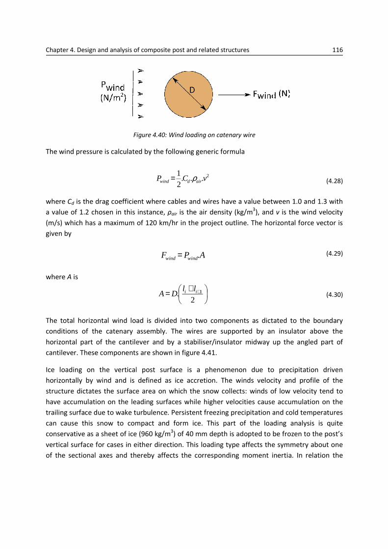
Chapter 4. Design and analysis of composite post and related structures
Figure
The wind pressure is calculated by the following generic formula
where Cd is the drag coefficient where cables and wires have a value between 1.0 and 1.3 with
a value of 1.2 chosen in this instance,
(m/s) which has a maximum of 120 km/hr in the project outline. The horizontal force vector is
given by
where A is
The total horizontal wind load is divided into two components as dictated to the boundary
conditions of the catenary assembly. The wires are supported by an insulator above the
horizontal part of the cantilever and by a stabiliser/insulator midway up the a
cantilever. These components are shown in figure 4
Ice loading on the vertical post surface is a phenomenon due to precipitation driven
horizontally by wind and is defined as ice accretion
structure dictates the surface area on which the snow collects: winds of low velocity tend to
have accumulation on the leading surfaces while higher velocities cause accumulation on the
trailing surface due to wake turbulence. Persistent freezing precipitation and c
can cause this snow to compact and form ice. This part of the loading analysis is quite
conservative as a sheet of ice (960 kg/m
vertical surface for cases in either direction. This lo
of the sectional axes and thereby affects the corresponding mom
of composite post and related structures
Figure 4.40: Wind loading on catenary wire
The wind pressure is calculated by the following generic formula
2...21
vCP airdwind ρ=
is the drag coefficient where cables and wires have a value between 1.0 and 1.3 with
his instance, ρair is the air density (kg/m3), and
(m/s) which has a maximum of 120 km/hr in the project outline. The horizontal force vector is
APF windwind .=
+= +
2. 1ii ll
DA
The total horizontal wind load is divided into two components as dictated to the boundary
conditions of the catenary assembly. The wires are supported by an insulator above the
horizontal part of the cantilever and by a stabiliser/insulator midway up the a
cantilever. These components are shown in figure 4.41.
Ice loading on the vertical post surface is a phenomenon due to precipitation driven
and is defined as ice accretion. The winds velocity and profile of the
dictates the surface area on which the snow collects: winds of low velocity tend to
have accumulation on the leading surfaces while higher velocities cause accumulation on the
trailing surface due to wake turbulence. Persistent freezing precipitation and c
can cause this snow to compact and form ice. This part of the loading analysis is quite
conservative as a sheet of ice (960 kg/m3) of 40 mm depth is adopted to be frozen to the post’s
vertical surface for cases in either direction. This loading type affects the symmetry about one
of the sectional axes and thereby affects the corresponding moment inertia. In relation the
116
(4.28)
is the drag coefficient where cables and wires have a value between 1.0 and 1.3 with
), and v is the wind velocity
(m/s) which has a maximum of 120 km/hr in the project outline. The horizontal force vector is
(4.29)
(4.30)
The total horizontal wind load is divided into two components as dictated to the boundary
conditions of the catenary assembly. The wires are supported by an insulator above the
horizontal part of the cantilever and by a stabiliser/insulator midway up the angled part of
Ice loading on the vertical post surface is a phenomenon due to precipitation driven
. The winds velocity and profile of the
dictates the surface area on which the snow collects: winds of low velocity tend to
have accumulation on the leading surfaces while higher velocities cause accumulation on the
trailing surface due to wake turbulence. Persistent freezing precipitation and cold temperatures
can cause this snow to compact and form ice. This part of the loading analysis is quite
) of 40 mm depth is adopted to be frozen to the post’s
ading type affects the symmetry about one
ent inertia. In relation the
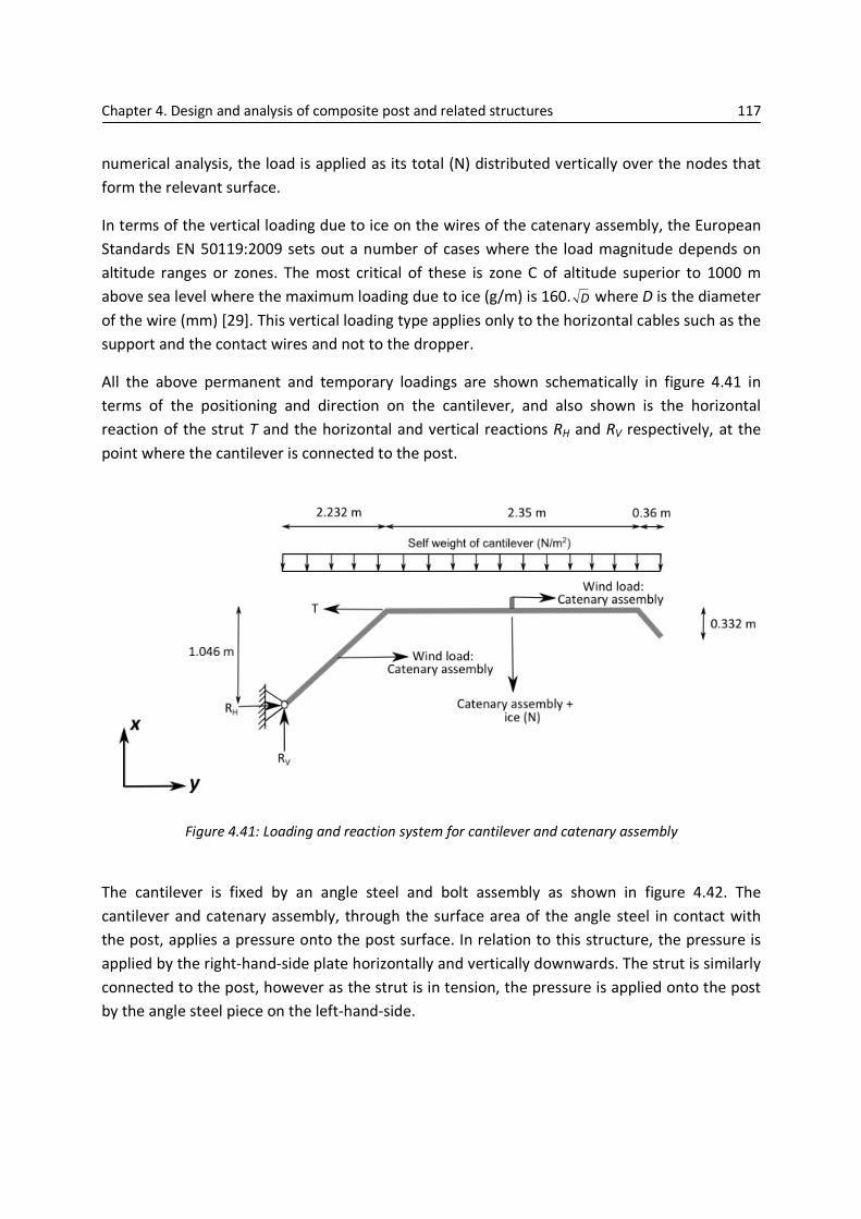
Chapter 4. Design and analysis of composite post and related structures 117
numerical analysis, the load is applied as its total (N) distributed vertically over the nodes that
form the relevant surface.
In terms of the vertical loading due to ice on the wires of the catenary assembly, the European
Standards EN 50119:2009 sets out a number of cases where the load magnitude depends on
altitude ranges or zones. The most critical of these is zone C of altitude superior to 1000 m
above sea level where the maximum loading due to ice (g/m) is 160. D where D is the diameter
of the wire (mm) [29]. This vertical loading type applies only to the horizontal cables such as the
support and the contact wires and not to the dropper.
All the above permanent and temporary loadings are shown schematically in figure 4.41 in
terms of the positioning and direction on the cantilever, and also shown is the horizontal
reaction of the strut T and the horizontal and vertical reactions RH and RV respectively, at the
point where the cantilever is connected to the post.
Figure 4.41: Loading and reaction system for cantilever and catenary assembly
The cantilever is fixed by an angle steel and bolt assembly as shown in figure 4.42. The
cantilever and catenary assembly, through the surface area of the angle steel in contact with
the post, applies a pressure onto the post surface. In relation to this structure, the pressure is
applied by the right-hand-side plate horizontally and vertically downwards. The strut is similarly
connected to the post, however as the strut is in tension, the pressure is applied onto the post
by the angle steel piece on the left-hand-side.
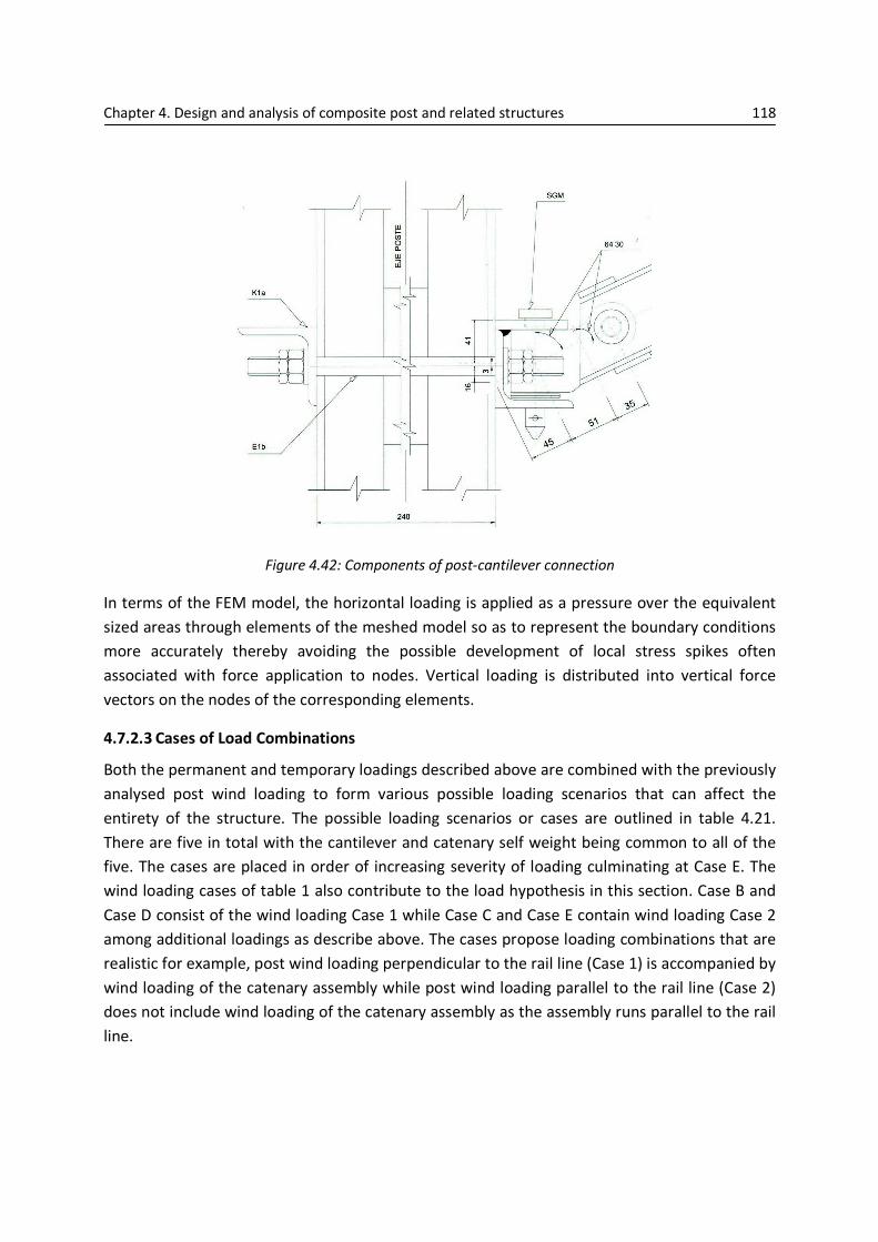
Chapter 4. Design and analysis of composite post and related structures 118
Figure 4.42: Components of post-cantilever connection
In terms of the FEM model, the horizontal loading is applied as a pressure over the equivalent
sized areas through elements of the meshed model so as to represent the boundary conditions
more accurately thereby avoiding the possible development of local stress spikes often
associated with force application to nodes. Vertical loading is distributed into vertical force
vectors on the nodes of the corresponding elements.
4.7.2.3 Cases of Load Combinations
Both the permanent and temporary loadings described above are combined with the previously
analysed post wind loading to form various possible loading scenarios that can affect the
entirety of the structure. The possible loading scenarios or cases are outlined in table 4.21.
There are five in total with the cantilever and catenary self weight being common to all of the
five. The cases are placed in order of increasing severity of loading culminating at Case E. The
wind loading cases of table 1 also contribute to the load hypothesis in this section. Case B and
Case D consist of the wind loading Case 1 while Case C and Case E contain wind loading Case 2
among additional loadings as describe above. The cases propose loading combinations that are
realistic for example, post wind loading perpendicular to the rail line (Case 1) is accompanied by
wind loading of the catenary assembly while post wind loading parallel to the rail line (Case 2)
does not include wind loading of the catenary assembly as the assembly runs parallel to the rail
line.
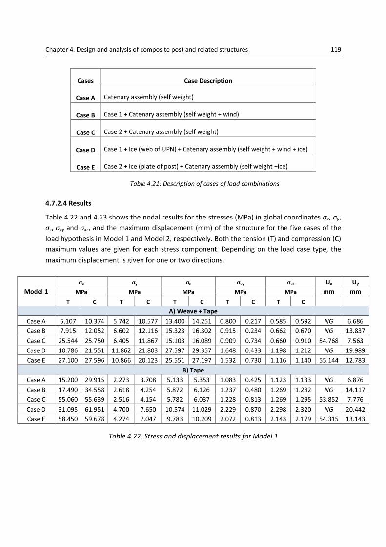
Chapter 4. Design and analysis of composite post and related structures 119
Cases Case Description
Case A Catenary assembly (self weight)
Case B Case 1 + Catenary assembly (self weight + wind)
Case C Case 2 + Catenary assembly (self weight)
Case D Case 1 + Ice (web of UPN) + Catenary assembly (self weight + wind + ice)
Case E Case 2 + Ice (plate of post) + Catenary assembly (self weight +ice)
Table 4.21: Description of cases of load combinations
4.7.2.4 Results
Table 4.22 and 4.23 shows the nodal results for the stresses (MPa) in global coordinates σx, σy,
σz, σxy and σxz, and the maximum displacement (mm) of the structure for the five cases of the
load hypothesis in Model 1 and Model 2, respectively. Both the tension (T) and compression (C)
maximum values are given for each stress component. Depending on the load case type, the
maximum displacement is given for one or two directions.
σx σy σz σxy σxz Uz Uy
Model 1 MPa MPa MPa MPa MPa mm mm
T C T C T C T C T C
A) Weave + Tape
Case A 5.107 10.374 5.742 10.577 13.400 14.251 0.800 0.217 0.585 0.592 NG 6.686
Case B 7.915 12.052 6.602 12.116 15.323 16.302 0.915 0.234 0.662 0.670 NG 13.837
Case C 25.544 25.750 6.405 11.867 15.103 16.089 0.909 0.734 0.660 0.910 54.768 7.563
Case D 10.786 21.551 11.862 21.803 27.597 29.357 1.648 0.433 1.198 1.212 NG 19.989
Case E 27.100 27.596 10.866 20.123 25.551 27.197 1.532 0.730 1.116 1.140 55.144 12.783
B) Tape
Case A 15.200 29.915 2.273 3.708 5.133 5.353 1.083 0.425 1.123 1.133 NG 6.876
Case B 17.490 34.558 2.618 4.254 5.872 6.126 1.237 0.480 1.269 1.282 NG 14.117
Case C 55.060 55.639 2.516 4.154 5.782 6.037 1.228 0.813 1.269 1.295 53.852 7.776
Case D 31.095 61.951 4.700 7.650 10.574 11.029 2.229 0.870 2.298 2.320 NG 20.442
Case E 58.450 59.678 4.274 7.047 9.783 10.209 2.072 0.813 2.143 2.179 54.315 13.143
Table 4.22: Stress and displacement results for Model 1

Chapter 4. Design and analysis of composite post and related structures 120
σx σy σz σxy σxz Uz Uy
Model 2 MPa MPa MPa MPa MPa mm mm
T C T C T C T C T C
A) Weave + Tape
Case A 4.379 8.432 4.201 8.089 10.538 11.335 0.850 0.393 0.462 0.465 NG 5.755
Case B 7.023 9.785 4.830 9.255 12.049 12.963 1.022 0.379 0.522 0.526 NG 12.083
Case C 41.885 46.247 12.168 12.592 11.876 12.592 2.918 3.436 0.520 1.365 61.596 6.509
Case D 9.290 17.505 8.678 16.673 21.701 23.347 1.801 0.739 0.945 0.953 NG 17.378
Case E 43.613 48.789 12.322 15.218 20.091 21.631 2.818 3.618 0.880 1.400 61.977 11.002
B) Tape
Case A 12.755 25.937 1.577 2.888 4.256 4.469 1.195 0.547 0.938 0.974 NG 6.149
Case B 15.840 29.921 1.812 3.313 4.868 5.113 1.437 0.530 0.020 0.020 NG 12.858
Case C 92.593 102.480 2.674 3.231 4.795 5.043 3.777 4.469 1.059 1.268 60.522 6.951
Case D 26.093 53.671 3.251 5.958 8.767 9.206 2.532 1.031 1.920 1.940 NG 18.516
Case E 96.663 108.540 2.951 5.483 8.113 8.525 3.557 4.723 1.790 1.822 60.574 11.749
Table 4.23: Stress and displacement results for Model 2
From observation of the above results, the largest displacement change experienced occurs for
in the y-direction (towards the rail line) caused by Case D. For both Model 1 and Model 2
subjected to load Case D, the displacement increases 3.14 times from that experienced for load
Case 1 of tables 4.9 and 4.10 However, this increase is still relatively small with only a
magnitude change of 13.942 mm and 12.636 mm for Models 1 and 2, respectively.
The introduction of the cantilever and contributing loads from the catenary assembly creates
new load conditions on the structure. Recalling the loading-reaction diagram of figure 4.35, the
resultant forces from the post-cantilever connection can be represented as those in the figure
below where T is the horizontal strut force and FH and FV represent the horizontal and vertical
force components at the pin joint of the cantilever. Both the horizontal forces T and FH are
applied as pressures over a region of elements that simulate the post-cantilever connection
shown in figure 4.43. Often such loads can be applied as forces directly to a node set however
local stress concentrations can occur as a result. On the other hand, the application of the
equivalent pressure over a set of elements reduces this undesired stress spiking effect. Finally,
the vertical force component FV is applied to the nodes that make up the element set on which
the FH force component is applied as a pressure.

Chapter 4. Design and analysis of composite post and related structures 121
Figure 4.43: Stress concentrations (σx) at post-cantilever connection
The application of loading combinations in directions parallel and perpendicular to the rail line
causes the post to suffer a twisting effect as can be observed from the stress distribution (σx)
diagram of the structure below in figure 4.44. Such loading combinations are found in Case C
and Case E where the wind pressure is parallel to the rail line and the self-weight of the
catenary assembly causes a moment about the z-axis at the top of the structure. The stress
variation across the post section is captured graphically in figure 4.45. As before, the section is
taken 40 mm above the fixed end making again the sketch of the section in figure 4.13
applicable in this instance. The stress path demonstrates the effects caused by the twisting in
the section where the stress variation is not symmetrical about the centre of the post’s width as
was observed for load Case 2 in figure 4.15.
T
FH
Fv
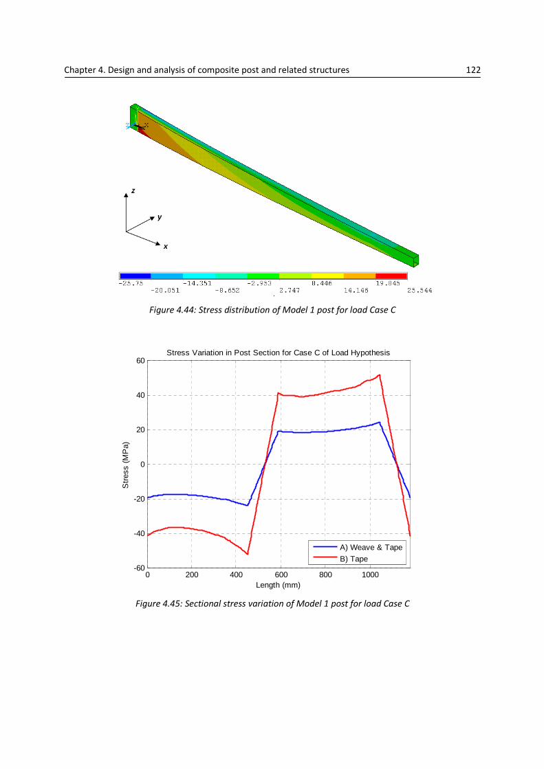
Chapter 4. Design and analysis of composite post and related structures 122
Figure 4.44: Stress distribution of Model 1 post for load Case C
Figure 4.45: Sectional stress variation of Model 1 post for load Case C
0 200 400 600 800 1000-60
-40
-20
0
20
40
60
Length (mm)
Str
ess
(MP
a)
Stress Variation in Post Section for Case C of Load Hypothesis
A) Weave & Tape
B) Tape

Chapter 4. Design and analysis of composite post and related structures 123
4.8 Design and Analysis of a Proposed Steel Moment Base
The proceeding section details the intermediate design-analysis of the moment resistant base
accompanying the composite post structure. This type of mechanical fixation was chosen above
other types for the following reasons
� New concrete foundation not required
� Rapid mounting and dismounting process of post
� Relatively light, can be carried manually
� Relatively cheap fabrication costs
� Reusable
� Can be designed and analysed with a high level of accuracy.
As briefly described in Section 4.1.2, the proposed composite post differs from the original steel
post in terms of its method of fixation which subsequently alters the overall height of the
structure and the boundary conditions imposed. The proposed structural fixation consists of
mounting the post onto the top of the original post’s concrete foundation by the steel moment
resistant base. The base itself is secured to the concrete pad and to the composite post by bolt
connections. The model brings together three different element types with the motivation for
their implentation and their description outlined below.
4.8.1 Proposed Base Description
The base’s preliminary design is based on the classical moment resistant base design for post
type structures where overturning of the structure is impeded by plate components fixed
transversally to the axis of overturning. Carbon steel S275JR similar to the original post, is the
material of choice because of its mechanical properties as outlined previously in table 3.3 of the
original steel post analysis. Steel was also chosen for the relative ease in which it can be
fabricated into complex mechanical structures including. Figure 4.46 shows an image of the
proposed base structure developed in the numerical model. Also included are the separate area
components which determine the required meshing characteristics in the latter stages.

Chapter 4. Design and analysis of composite post and related structures 124
Figure 4.46: Image of proposed steel base taken from the numerical model
The geometry of the structure is shown as CAD drawings below in figures 4.47 to 4.49. The
main features of the base include a flat plate in contact with the surface of the foundation,
vertical thin-walled section at a height of 200 mm and an inner section with the ‘equivalent’
outer dimensions of the post structure. The word equivalent is used with caution as the inner
dimension of the vertical walls of the base are fabricated to the same outer dimensions of the
post plus a tolerance. This extra-dimensional tolerance factors in discrepancies that come about
during fabrication, these include residual stresses and therefore deformations experienced in
the steel base caused during fabrication (welding and cutting), and deformations and
curvatures in the composite post which can occur during the curing process as a result of
unsymmetrical laminates, and fibre alignment discrepancies.
As already mentioned above, the base includes plate components connected at their thickness
to the vertical wall face and to the horizontal plate. The majority of moment resistance in the
structure is provided by these plates. In terms of dimensions, the plate component has a width
of 75 mm which tapers at one side inwards towards its height of 150 mm. These moment plates
are fabricated such that the taper does not reach its bottom or top. This ‘blunting’ of the taper
removes the likely occurrence, during loading, of stress concentrations of infinitesimal
magnitudes caused by severe geometric discontinuities. Bolt holes in the horizontal plate are
situated outside the section wall and between the moment plates. In total, there are ten bolt
holes in the horizontal plate. The bolt holes that connect the base and post are situated in the
base’s vertical walls spaced between the moment plates. Each of the longitudinal and
transversal walls consists of four and two bolts holes, respectively.

Chapter 4. Design and analysis of composite post and related structures 125
Figure 4.47: Longitudinal view of moment resistant base
Figure 4.48: Transversal view of moment resistant base
Figure 4.49: Plan view of moment resistant base

Chapter 4. Design and analysis of composite post and related structures 126
4.8.2 Finite Element Model
The steel base is considered as a solid structure. The SOLID45 element is therefore
implemented as it is appropriately used for the 3-D modelling of solid structures. This solid first-
order element is defined by eight nodes having three degrees of freedom at each node:
translations in the nodal x, y, and z directions. The elements attributes include plasticity, creep,
swelling, stress stiffening, large deflection, and large strain capabilities. Figure 4.50 depicts the
solid element with its local and surface coordinate systems included.
Figure 4.50: 8-node SOLID45 element
As can be seen in the above figure, the geometry of the element is defined by its eight nodes
with its coordinate system directly related to the configuration of the nodes. Accuracy of the
model is enhanced by solving the system by full integration (KEYOPT(2) = 0) with extra
displacement shapes (KEYOPT(1) = 0) although it is more CPU intensive. The full integration
analysis allows the capture of bending behaviour of single layer elements [8].
4.8.3 Model Development Method
Before the model can be analysed, a number of assumptions and limitations are defined at its
design stage. Complexity arises in attempting to best approximate the boundary conditions of
the structure, i.e. the base’s interaction with the foundation and post. The composite post
structure is therefore modelled in the analysis with its relevant boundary conditions included,
i.e. wind loading over its free surface. The inclusion of a second mechanical structure in the
design-analysis stage introduces a number of additional issues that require clarification. These
are dealt with by means of imposing assumptions and limitations onto the model. These include
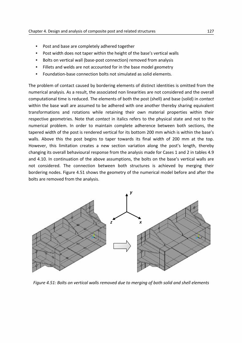
Chapter 4. Design and analysis of composite post and related structures 127
• Post and base are completely adhered together
• Post width does not taper within the height of the base’s vertical walls
• Bolts on vertical wall (base-post connection) removed from analysis
• Fillets and welds are not accounted for in the base model geometry
• Foundation-base connection bolts not simulated as solid elements.
The problem of contact caused by bordering elements of distinct identities is omitted from the
numerical analysis. As a result, the associated non linearities are not considered and the overall
computational time is reduced. The elements of both the post (shell) and base (solid) in contact
within the base wall are assumed to be adhered with one another thereby sharing equivalent
transformations and rotations while retaining their own material properties within their
respective geometries. Note that contact in italics refers to the physical state and not to the
numerical problem. In order to maintain complete adherence between both sections, the
tapered width of the post is rendered vertical for its bottom 200 mm which is within the base’s
walls. Above this the post begins to taper towards its final width of 200 mm at the top.
However, this limitation creates a new section variation along the post’s length, thereby
changing its overall behavioural response from the analysis made for Cases 1 and 2 in tables 4.9
and 4.10. In continuation of the above assumptions, the bolts on the base’s vertical walls are
not considered. The connection between both structures is achieved by merging their
bordering nodes. Figure 4.51 shows the geometry of the numerical model before and after the
bolts are removed from the analysis.
Figure 4.51: Bolts on vertical walls removed due to merging of both solid and shell elements

Chapter 4. Design and analysis of composite post and related structures 128
As this design-analysis is considered to be at an intermediate stage, modelling details such as
fillet and weld components are not taken into account in the geometry due to their time-
consuming formation. The omission of such components creates stress concentration issues at
the areas of geometric discontinuity. Such behavioural responses occurring in the results stage
of the analysis are distinguished and recognised.
Finally, the issue of modelling the bolt assembly arises at the base-foundation connection.
Figure 4.52 shows two typical base connection and bolt assembly relevant to this design-
analysis.
Figure 4.52: Sectional view of bolt assembly for base-foundation connection
There are numerous methods to simulate the bolt assembly which include a complete solid
bolt, hybrid bolt, spider bolt, Rigid Body Element (RBE) bolt, coupled bolt, and no-bolt
simulation, with each method varying in their degree of accuracy. The most accurate approach
is to model the complete 3D solid bolt assembly however, with regards to the present analysis,
a large number of bolt assemblies are required (10 in total) and as a result, modelling of solid
bolts is impractical. Therefore, the analysis of the bolt assembly is carried out using line
elements (LINK10) and coupled nodes. This method reduces drastically the number of elements
required in the bolt assembly analysis with the LINK10 element adequately simulating the nut.
The typical bolt joint assembly and its numerical model equivalent are shown in figure 4.53.

Chapter 4. Design and analysis of composite post and related structures 129
Figure 4.53: Numerical model representation of bolt assembly
The figure above shows the bolt element (LINK10) passing through the bolt hole and coupled to
surface nodes that represent the contact area between the head of the bolt and the base plate.
The LINK10 element is a 3-D spar element with three degrees of freedom at each node
(translations x, y, and z directions). The element simulates the nut of the bolt assembly which
has uniaxial tension capabilities only. The head is represented by coupled nodes. Coupling is
carried out between the outermost node of the LINK10 element (master node) and the
circumferential nodes of the flange at the hole (slave nodes). These circumferential nodes are
created by defining separate circular areas around the holes during the model development
and are mapped meshed. The bottom node of the link element simulates the point at which the
bolt enters the foundation. The displacement at this node is impeded.
In order to perform the iterative process of design, a number of the design drivers were defined
parametrically in the numerical input code of the model. Design drivers of the base structure
include the thickness of the horizontal base plate, the walls, and the moment plates which are
all defined separately. Also included as parameters are the bolt hole size and the area of the
bolt head in contact with the base. After completing the iterative design process, it was
determined that for the analysis stage the thickness parameters of the horizontal base plate
and the walls/moment plate would be equal to 9 mm and 7 mm, respectively.
Master Node
Base surface in
contact with bolt
Link Element
Slave Nodes
Plate thickness

Chapter 4. Design and analysis of composite post and related structures 130
Taking into account that the steel base structure has two planes of symmetry, it is initially
modelled as one-quarter of its entire size. Due to the base’s isotropic properties, the REFLECT
command is adequately used in terms of overall time reduction in the geometric and meshing
development of the solid element. Figure 4.54 describes the progression of the model’s
development from one-quarter to complete structure using the REFLECT command.
Figure 4.54: One-quarter and complete structure
However, the REFLECT command is not utilised for the shell element structure (i.e. the
composite laminates of the post) due to its anisotropic nature. This command would create
conflicting lamina configurations at areas either side of the planes of symmetry. In order to
merge the nodes of both element types at the interface of the base/post, the elements of both
structures must be identical in the areas of contact. To achieve this, the complete base
developed and meshed, a copy of the keypoints at the base’s internal vertical surface (in
contact with composite laminates) is made at their same location. The shell areas and their
orientation are defined by these new keypoints and their sequence (i, j, k, l). The newly meshed
SHELL181 elements are dimensionally identical as to those of their corresponding SOLID45
elements. Figure 4.55 shows firstly the complete meshed base model (grey) and secondly the
coinciding meshed shell areas (green) of the post that adjoin the interior faces of the base’s
walls.

Chapter 4. Design and analysis of composite post and related structures 131
Figure 4.55: Complete meshed base model and coinciding meshed shell areas of the post
Figure 4.56 shows the meshed base and included in its interior is the section of the meshed
post that is merged with the base which effectively anchors the post. Also shown are the
stacked layers that create the UPN beam and plate laminate components of the post.
Figure 4.56: Meshed base plus meshed post section joined to base
Meshed shell areas of post

Chapter 4. Design and analysis of composite post and related structures 132
The remaining length of the composite post is created in the same manner as described
previously in the method statement of Section 4.2.2. As the base structure is of the most
importance in this analysis, the unconstrained post length is coarsely meshed so as to
reduce computational time. While the meshing maybe relatively coarse, the response
obtained remains at a high degree of accuracy in its approximation due to the full
integration option for the SHELL181 element used in the analysis (KEYOPT(3) = 2). Figure
4.51 shows a segment of the coarsely meshed unconstrained post (green) connected to the
finely meshed post segment contained within the base structure.
Figure 4.57: Base-post connection for numerical model
4.8.4 Boundary Conditions and loads
The loading applied in this analysis consists of the two distinct load-direction cases in table 1. As
the loading simulates wind, it is also applied over the relevant areas of the base structure as
well as the post. The boundary conditions at the base-foundation connection (plate component
at y-z plane) vary with the case type. The boundary conditions for each case are divided into
two situations which are defined by their location either side of the axis of rotation. The base
area on the side at which the load is originating from can be defined as the ‘lift’ zone as the
base plate in this area is simulating separation from the foundation while the other area is
pressing down onto the foundation. The base plate area segments of the ‘lift’ zone are not
constrained allowing them to translate and rotate as is the case in the actual base-foundation
connection. The area segments on the other side of the axis of rotation are constrained in

Chapter 4. Design and analysis of composite post and related structures 133
translation and rotation so as to prevent them ‘pushing’ down into the foundation. As
previously described, all the bolts are constrained by the bottom node of the LINK10 element.
4.8.5 Results
The most significant stress and displacement results are shown in table 4.24 below. They
include principal stress σ1, σ2, and σ3, and Von Mises equivalent stress.
Case σ1 σ2 σ3 Von Mises Displacement
MPa MPa MPa MPa mm
1 87.869 41.847 27.174 75.461 0.030
2 232.52 102.10 72.910 196.30 0.110
Table 4.24: Principal stresses maximums and equivalent Von Mises stresses
The final bolt assembly dimensions are shown in figure 4.58 and were determined from the
British Standard Whitworth (BSW) system. The bolt is of Grade A2/A4 - DIN 965 – DIN EN ISO
7046-2. The assembly includes also a lock nut which resists loosening under vibration by locking
the first nut in position. An alternative method to prevent loosening is to utilise only one nut
which has a nylon sleeve insert. As the nut is fed and tightened onto the bolt the thread cuts
into the nylon thereby holding the assembly together by means of friction.
Figure 4.58: Bolt assembly dimensions (Whitworth System)
Table 4.25 lists the reaction forces of the bolts for both load cases. A slight pretension is applied
to the bolts before the solution phase of the numerical model so as to simulate a tight bolt
assembly. The results are given as reaction force and tonnes.
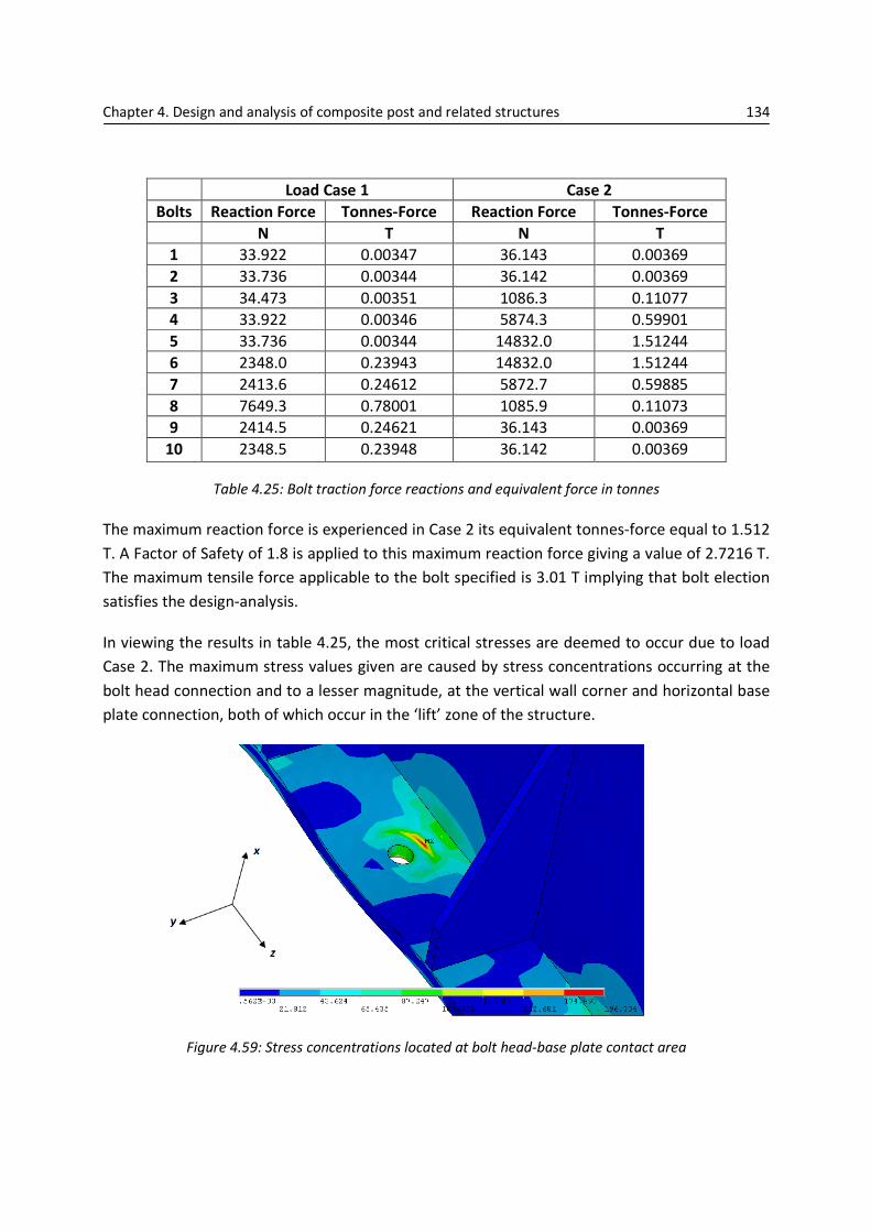
Chapter 4. Design and analysis of composite post and related structures 134
Load Case 1 Case 2
Bolts Reaction Force Tonnes-Force Reaction Force Tonnes-Force
N T N T
1 33.922 0.00347 36.143 0.00369
2 33.736 0.00344 36.142 0.00369
3 34.473 0.00351 1086.3 0.11077
4 33.922 0.00346 5874.3 0.59901
5 33.736 0.00344 14832.0 1.51244
6 2348.0 0.23943 14832.0 1.51244
7 2413.6 0.24612 5872.7 0.59885
8 7649.3 0.78001 1085.9 0.11073
9 2414.5 0.24621 36.143 0.00369
10 2348.5 0.23948 36.142 0.00369
Table 4.25: Bolt traction force reactions and equivalent force in tonnes
The maximum reaction force is experienced in Case 2 its equivalent tonnes-force equal to 1.512
T. A Factor of Safety of 1.8 is applied to this maximum reaction force giving a value of 2.7216 T.
The maximum tensile force applicable to the bolt specified is 3.01 T implying that bolt election
satisfies the design-analysis.
In viewing the results in table 4.25, the most critical stresses are deemed to occur due to load
Case 2. The maximum stress values given are caused by stress concentrations occurring at the
bolt head connection and to a lesser magnitude, at the vertical wall corner and horizontal base
plate connection, both of which occur in the ‘lift’ zone of the structure.
Figure 4.59: Stress concentrations located at bolt head-base plate contact area

Chapter 4. Design and analysis of composite post and related structures 135
Figure 4.60: Stress concentrations located at wall-base plate connection
While it is accepted that both types of stress concentrations occur at these regions, they are
however viewed as being overestimations of the actual stresses incurred. The overestimation of
the stress magnitudes are a result of a number of the limitations outlined at the beginning of
the base design. Two of which are of most relevance are recalled as being
• Foundation-base connection bolts not simulated as solid elements
• Fillets and welds are not accounted for in the base model geometry.
The stress response for both limitations is shown above in figures 4.59 and 4.60. The method of
the nodal coupling used to represent the bolt assembly has its limitations. All translations and
rotations of the coupled nodes which represent the bolt head in contact with the base are
completely constrained. This in turn causes high local stresses in its proximate unconstrained
region. The severe change in geometry at the wall-base plate interface of the model is reduced
by the presence of welded connections between the two.
Figures 4.61 and 4.62 show the stress distribution and deformed shape of the base structure for
load Case 2. It must be highlighted that the displacement scale is amplified and the stress range
is reduced in order to appreciate the behavioural response. A number of interesting
observations can be made from figure 4.55 which include the sectional shape of the walls and
the response of the moment connections. The inward deformation of the bottom wall is
connected to the composite post width in compression while conversely the top wall is adhered
to the post area in tension. Consequently, the outer moment plates connected to the
longitudinal walls are forced into flexure while the centre moment plate, which coincides with
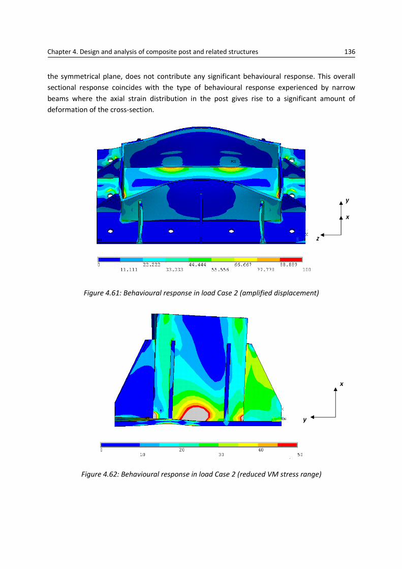
Chapter 4. Design and analysis of composite post and related structures 136
the symmetrical plane, does not contribute any significant behavioural response. This overall
sectional response coincides with the type of behavioural response experienced by narrow
beams where the axial strain distribution in the post gives rise to a significant amount of
deformation of the cross-section.
Figure 4.61: Behavioural response in load Case 2 (amplified displacement)
Figure 4.62: Behavioural response in load Case 2 (reduced VM stress range)
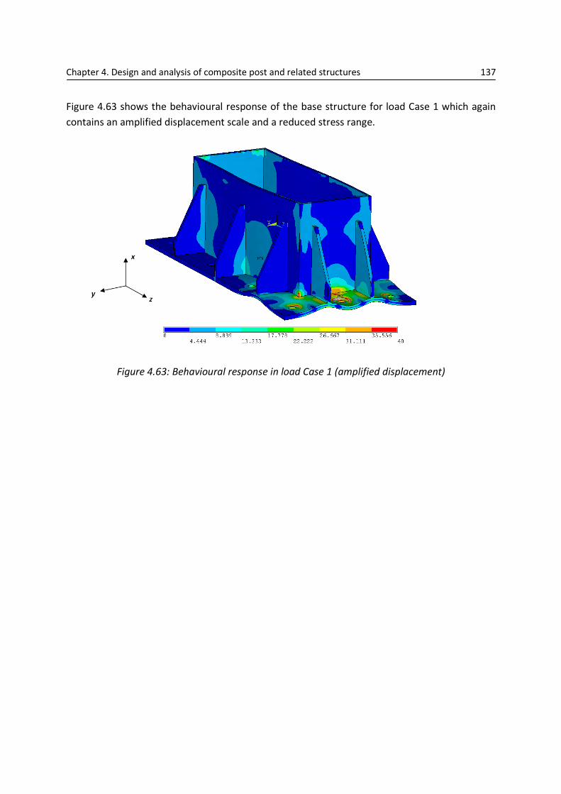
Chapter 4. Design and analysis of composite post and related structures 137
Figure 4.63 shows the behavioural response of the base structure for load Case 1 which again
contains an amplified displacement scale and a reduced stress range.
Figure 4.63: Behavioural response in load Case 1 (amplified displacement)

Chapter 4. Design and analysis of composite post and related structures 138


![Design, analysis and development of composite spur gear ......engine, fuel pumps, washing machine [1]. P.B. Pawara et al. have proposed analysis of composite material spur gear under](https://static.fdocuments.net/doc/165x107/6115564efd84c22cd0779d23/design-analysis-and-development-of-composite-spur-gear-engine-fuel-pumps.jpg)


