Chapter 3Chapter 3

Steady-State,O Di i l C d tiOne-Dimensional Conduction

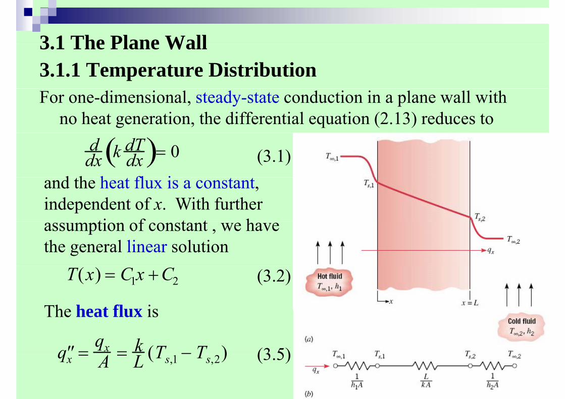
3 1 The Plane Wall3.1 The Plane Wall3.1.1 Temperature DistributionFor one-dimensional, steady-state conduction in a plane wall with

no heat generation, the differential equation (2.13) reduces toddx k dT

dx( )= 0

d h h fl i(3.1)

and the heat flux is a constant, independent of x. With further

ti f t t hassumption of constant , we have the general linear solution

T(x) = C1x + C2 (3.2)

The heat flux isThe heat flux is

′ ′ q =qx = k (T − T ) (3 5) q x = A = L (Ts,1 Ts,2) (3.5)

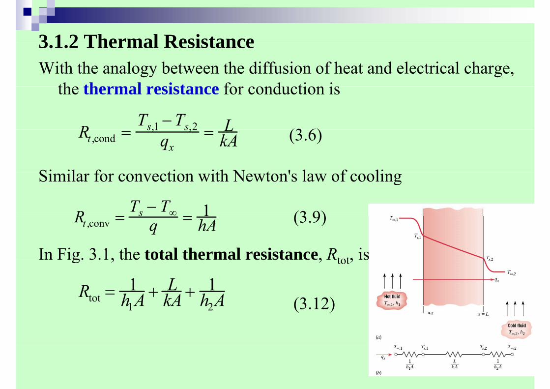
3 1 2 Thermal Resistance3.1.2 Thermal ResistanceWith the analogy between the diffusion of heat and electrical charge,

the thermal resistance for cond ction isthe thermal resistance for conduction is

RTs,1 − Ts,2 L (3 6)

Si il f ti ith N t ' l f li

Rt ,cond = s,1 s,2qx

= LkA (3.6)

Similar for convection with Newton's law of cooling

R Ts − T∞ 1 (3 9)

In Fig. 3.1, the total thermal resistance, Rtot, is

Rt ,conv = sq = hA (3.9)

In Fig. 3.1, the total thermal resistance, Rtot, is

Rtot = 1h A + L

kA + 1h A (3 12)h1A kA h2A (3.12)

3.1.3 The Composite Wall (Fig 3 2; Fig 3 3)3.1.3 The Composite Wall (Fig. 3.2; Fig. 3.3)

(3.19)Rtot = Rt∑ = ΔTq = 1

UAwhere U is the overall heat transfer coefficient, defined by

analogy to Newton's law of cooling asgy gqx ≡ UAΔT

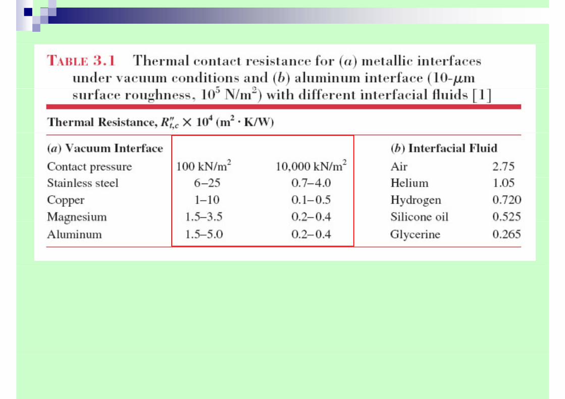
3 1 4 Contact Resistance3.1.4 Contact Resistance--significant temperature drop exists across an interface due to the

gaps bet een the contact areagaps between the contact areaContact resistance can be reduced by increasing the joint

d i h h f h i f l ipressure, reducing the roughness of the mating surfaces, applying a metal coating, inserting the interface with soft metal foil, or filli fl id f l th l d ti it t S T bl 3 1 dfilling fluid of large thermal conductivity, etc. See Tables 3.1 and 3.2.

EX 3.1, 3.2, 3.3

3 3 Radial Systems3.3 Radial Systems3.3.1 The CylinderFor steady-state conditions with no heat generation, Eq. 2.20 is

reduced to1 d k dT( ) 0 (3 23)

The conduction heat transfer rate qr (not the heat flux ) is a

1r

ddr kr dT

dr( )= 0

′ ′ q r(3.23)

rconstant in the radial direction

q kA dT k(2πrL) dTqr = −kA dTdr = −k(2πrL) dT

dr

(3 24)The general solution of (3.23) is

(3.24)

An example is shown in Fig. 3.6. T(r ) = C1 ln r + C2 (3.25)

p g

T − T ⎛ ⎞ T(r ) =

Ts,1 − Ts,2ln(r1 / r2 ) ln r

r2

⎛ ⎝ ⎜

⎞ ⎠ ⎟ + Ts,2

(3 26)

qr =2πLk(Ts,1 − Ts,2 )

ln(r / r )

(3.26)

(3.27)ln(r2 / r1)

R =ln(r2 / r1)

(3 28)Rt ,cond = 2πLk (3.28)

The temperature distribution for a composite cylindrical wall is shown in Fig. 3.7.

EX 3.5

3 5 Conduction with Thermal Energy Generation3.5 Conduction with Thermal Energy Generation3.5.1 The Plane WallFor steady-state conditions with constant k and uniform energy

generation per unit volume, Eq. 2.16 becomes

02

2=+ k

qdx

Td &(3.39)

The general solution is

&21

2

2)( CxCxkqxT ++−=

Some examples are shown in Fig. 3.9.With heat generation the heat flux is gno longer independent of x.

EX 3.7

3 6 Heat Transfer from Extended Surfaces3.6 Heat Transfer from Extended SurfacesUse of fins to enhance heat transfer from a wall: Figs. 3.12-3.143.6.1 A General Conduction Analysis (Fig. 3.15)Through energy balance, we obtain

ddx Ac

dTdx( )− h

kdAsdx (T − T∞ ) = 0

or d2Tdx2 + 1

Ac

dAcdx

⎛ ⎝ ⎜

⎞ ⎠ ⎟ dT

dx − 1Ac

hk

dAsdx

⎛ ⎝ ⎜

⎞ ⎠ ⎟ (T − T∞) = 0 (3.61)

3.6.2 Fins of Uniform Cross-Sectional Area

θ (0) = Tb − T∞ ≡ θb

3.6.2 Fins of Uniform Cross Sectional AreaWith dAc/dx = 0 and dAs/dx = P, Eq. 3.61 reduces to

d2T hP

Defining an excess temperature θ as

d2Tdx2 − hP

kAc(T − T∞ ) = 0

θ (x) ≡ T (x )− T∞

(3.62)

(3 63)g p ( ) ( ) ∞2

22 0d m

dxθ θ⇒ − = 2where

c

hPm kA≡ (3.64,65)

(3.63)

The general solution of (3.64) isdx c ( , )

θ(x) = C1emx + C2e−mx (3.66)

Two boundary conditions are needed. One boundary condition can be specified at the base of the fin (x = 0) as

θ (0) = Tb − T∞ ≡ θb( ) b ∞ b

The second condition may correspond to one of the four physicalThe second condition may correspond to one of the four physical situations shown in Table 3.4. The solution procedure to obtain temperature distribution θ/θb and fin heat transfer rate qf istemperature distribution θ/θb and fin heat transfer rate qf is discussed in the textbook.

EX 3.9

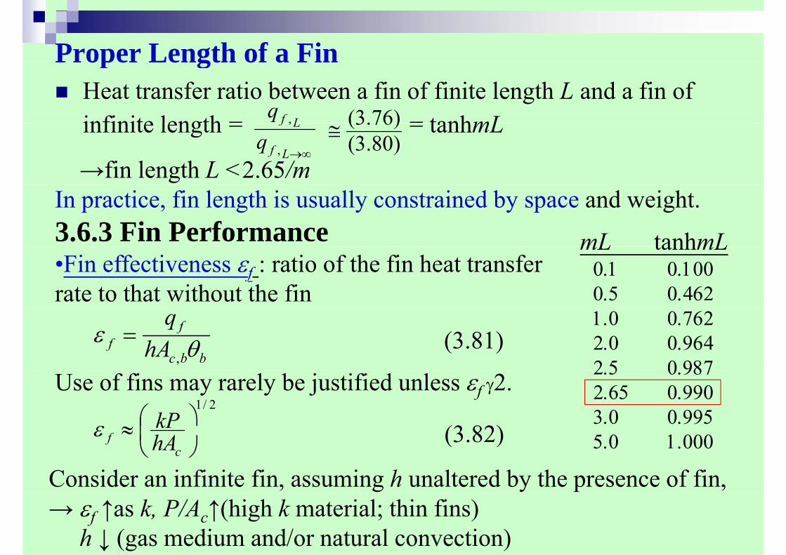
Proper Length of a FinProper Length of a FinHeat transfer ratio between a fin of finite length L and a fin of infinite length = = tanhmLLfq , )76.3(infinite length = = tanhmL

→fin length L <2.65/m∞→Lf

Lf

q ,

,

)80.3()76.3(≅

In practice, fin length is usually constrained by space and weight.

mL tanhmL3.6.3 Fin Performance mL tanhmL0.1 0.1000.5 0.462

•Fin effectiveness εf : ratio of the fin heat transfer rate to that without the fin

1.0 0.7622.0 0.9642 5 0 987bbc

ff hA

qθε

,= (3.81)

2.5 0.9872.65 0.9903.0 0.995

Use of fins may rarely be justified unless εf γ2.2/1

⎟⎞

⎜⎛≈ kPε (3 82) 5.0 1.000⎟

⎠⎜⎝

≈c

f hAε

Consider an infinite fin, assuming h unaltered by the presence of fin,

(3.82)

→ εf ↑as k, P/Ac↑(high k material; thin fins)h ↓ (gas medium and/or natural convection)

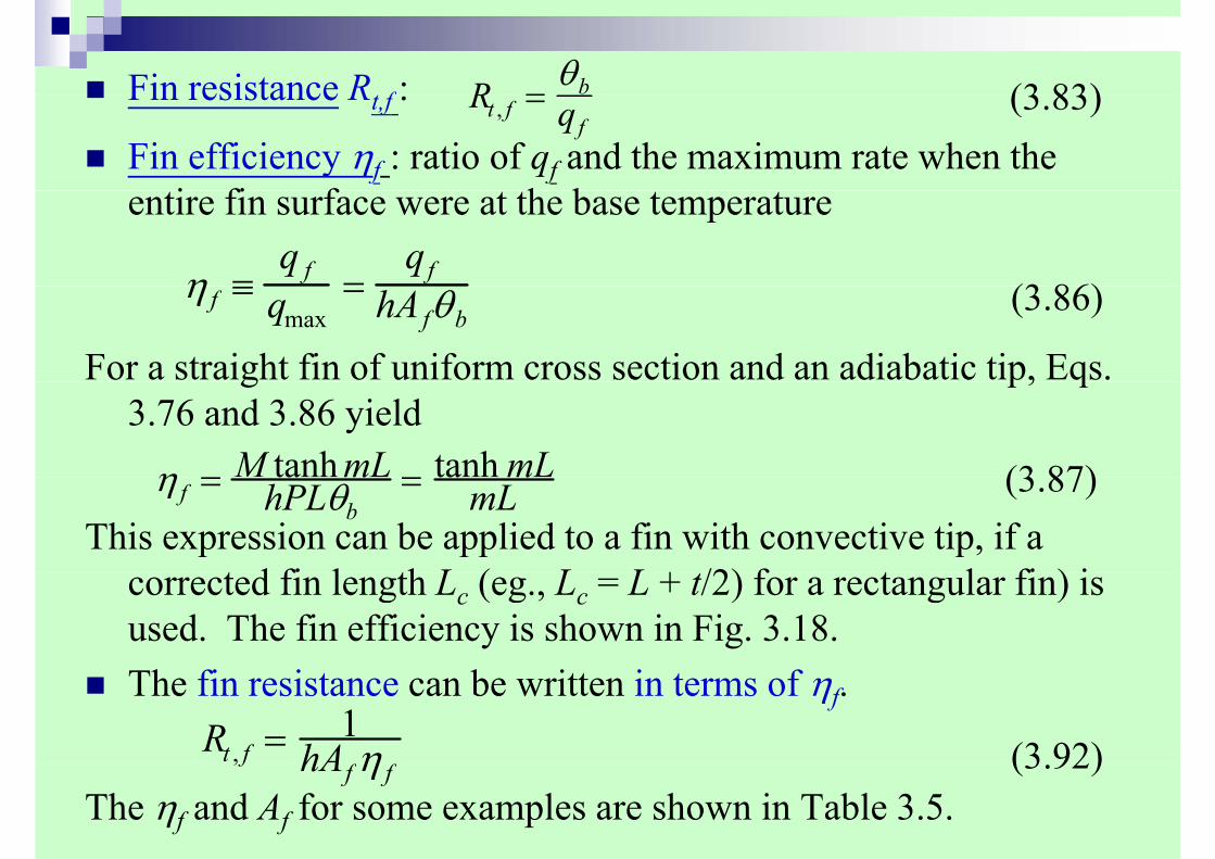
Fin resistance Rt f : R =θb (3 83)Fin resistance Rt,f :

Fin efficiency ηf : ratio of qf and the maximum rate when the i fi f h b

Rt , f = qf(3.83)

entire fin surface were at the base temperature

η ≡q f =

qf(3 86)

For a straight fin of uniform cross section and an adiabatic tip, Eqs.

η f ≡ qmax= hAfθb

(3.86)

g p, q3.76 and 3.86 yield

η M tanh mL tanh mL (3 87)This expression can be applied to a fin with convective tip, if a

t d fi l th L ( L L + /2) f t l fi ) i

η f = ta mhPLθb

= ta mmL (3.87)

corrected fin length Lc (eg., Lc = L + t/2) for a rectangular fin) is used. The fin efficiency is shown in Fig. 3.18.The fin resistance can be written in terms of ηf.

Rt , f = 1hA η (3 92)

The ηf and Af for some examples are shown in Table 3.5., f hAf η f (3.92)

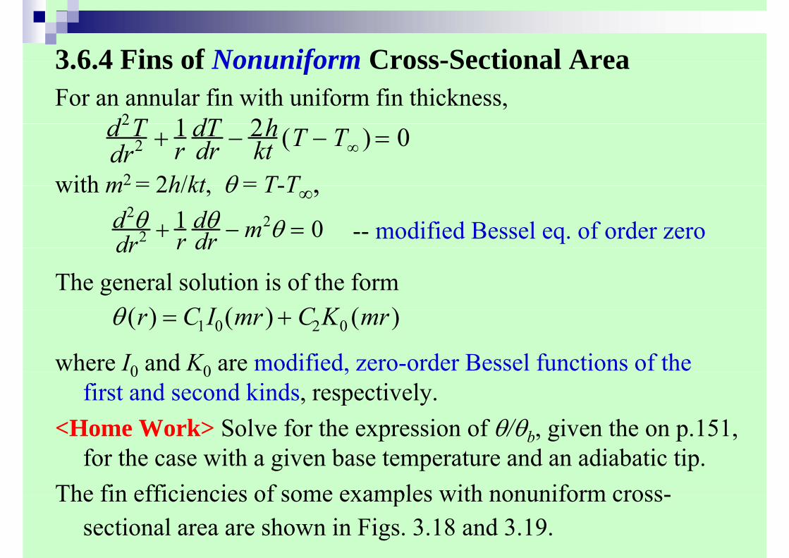
3 6 4 Fins of Nonuniform Cross-Sectional Area3.6.4 Fins of Nonuniform Cross-Sectional AreaFor an annular fin with uniform fin thickness,

d2T 1 dT 2h

with m2 = 2h/kt θ = T-T

d2Tdr2 + 1

rdTdr − 2h

kt (T − T∞ ) = 0

with m = 2h/kt, θ = T-T∞,d2θdr2 + 1

rdθdr − m2θ = 0 -- modified Bessel eq. of order zero

The general solution is of the formdr r dr

θ ( ) C I ( ) C K ( )

where I0 and K0 are modified, zero-order Bessel functions of the

θ (r) = C1I0(mr) + C2K0 (mr)

0 0 ,first and second kinds, respectively.

<Home Work> Solve for the expression of θ/θb, given the on p.151,<Home Work> Solve for the expression of θ/θb, given the on p.151, for the case with a given base temperature and an adiabatic tip.

The fin efficiencies of some examples with nonuniform cross-The fin efficiencies of some examples with nonuniform cross-sectional area are shown in Figs. 3.18 and 3.19.

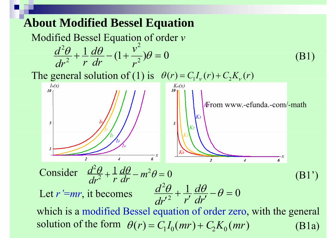
About Modified Bessel EquationAbout Modified Bessel EquationModified Bessel Equation of order v

22 1 (1 ) 0vd dθ θ θ (B1)2 21 (1 ) 0d dr drdr r

θ θ θ+ − + =

The general solution of (1) is 1 2( ) ( ) ( )r C I r C K rν νθ = +

(B1)

g ( ) 1 2( ) ( ) ( )ν ν

From www -efunda -com/-mathFrom www. efunda. com/ math

(B1’)Consider d2θdr2 + 1

rdθdr − m2θ = 0

2 1d dθ θLet r’=mr, it becomes2

21 0d dr drdr

θ θ θ+ − =′ ′′which is a modified Bessel equation of order zero with the generalwhich is a modified Bessel equation of order zero, with the general solution of the form θ (r) = C1I0(mr) + C2K0 (mr) (B1a)

221d dθ θCompare , having the general solution2

21 0d d mr drdr

θ θ θ+ − =

θ ( ) C I ( ) C K ( )

with (B2)2

2 0d mθ θ =

θ (r) = C1I0(mr) + C2K0 (mr) (B1a)

with (B2)2 0mdx

θ− =

which has the general solution

( ) mx mxθ

Since the modified Bessel equation corresponds to the(B2a)1 2( ) mx mxx C e C eθ −= +

Since the modified Bessel equation corresponds to the cylindrical coordinate, while (2) corresponds to the Cartesian coordinate their solutions are similar in trendCartesian coordinate, their solutions are similar in trend but (1a) reflects the effect of increasing surface area 2πrwith increasing rwith increasing r.

3 6 5 Overall Surface Efficiency3.6.5 Overall Surface Efficiency--characterizes an array of fins (Fig. 3.20) and the base surface to

hich the are attachedwhich they are attached

ηo =qt

q =qt

hA θ (3.98)

with At = NAf + Ab and qt = NηfhAfθb + hAbθb, we obtain

ηo qmax hAtθb( )

t f b t ηf f b b b

ηo = 1−NAfAt

(1− η f ) (3.102)

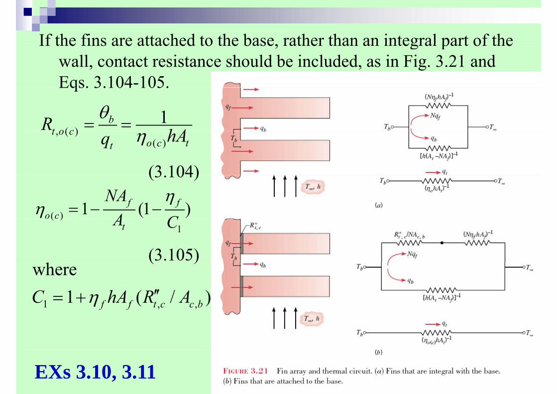
If the fins are attached to the base rather than an integral part of theIf the fins are attached to the base, rather than an integral part of the wall, contact resistance should be included, as in Fig. 3.21 and Eqs. 3.104-105.Eqs. 3.104 105.

ηo = 1 −NAfAt

(1 − η f )

( )1b

t o cR hAθ

= =, ( )( )

t o co c tt

hAq η

(3 104)

( ) 1 (1 )f fo c

NAA C

ηη = − −

(3.104)

( )1tA C

h(3.105)

1

where1 ( / )f f t c c bC hA R Aη ′′= +

( )

1 , ,( )f f t c c bη

EXs 3.10, 3.11