Chapter 3: Three faces of the derivative Overvieelyse/102/2017/Chap3.pdf · Chapter 3: Three faces...
181
Chapter 3: Three faces of the derivative Overview We already saw an algebraic way of thinking about a derivative.
Transcript of Chapter 3: Three faces of the derivative Overvieelyse/102/2017/Chap3.pdf · Chapter 3: Three faces...
Chapter 3: Three faces of the derivative
Overview
We already saw an algebraic way of thinking about a derivative.
Geometric: zooming into a line
Analytic: continuity and rational functions
Computational: approximations with computers

Chapter 3: Three faces of the derivative
Overview
We already saw an algebraic way of thinking about a derivative.
Geometric: zooming into a line
Analytic: continuity and rational functions
Computational: approximations with computers

Chapter 3: Three faces of the derivative
Overview
We already saw an algebraic way of thinking about a derivative.
Geometric: zooming into a line
Analytic: continuity and rational functions
Computational: approximations with computers

Chapter 3: Three faces of the derivative
Overview
We already saw an algebraic way of thinking about a derivative.
Geometric: zooming into a line
Analytic: continuity and rational functions
Computational: approximations with computers

Chapter 3: Three faces of the derivative 3.1 The geometric view: zooming into the graph of a function
Zooming In
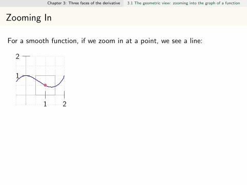
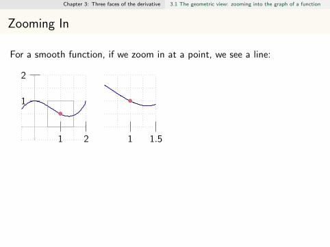
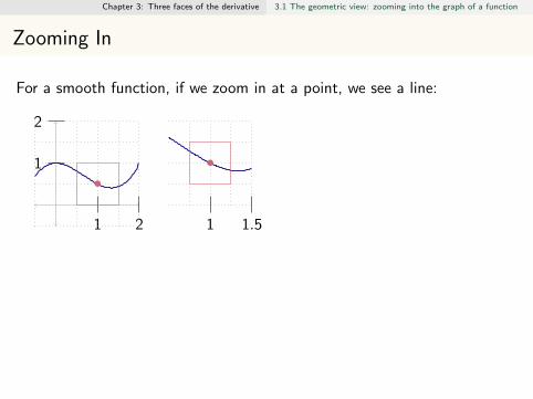
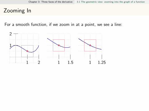
For a smooth function, if we zoom in at a point, we see a line:
•
1 2
1
2
•
1 1.5 1 1.25
• •
1 1.25
In this example, the slope of our zoomed-in line looks to be about:
∆y
∆x≈ −1
2
Chapter 3: Three faces of the derivative 3.1 The geometric view: zooming into the graph of a function
Zooming In
For a smooth function, if we zoom in at a point, we see a line:
•
1 2
1
2
•
1 1.5 1 1.25
• •
1 1.25
In this example, the slope of our zoomed-in line looks to be about:
∆y
∆x≈ −1
2
Chapter 3: Three faces of the derivative 3.1 The geometric view: zooming into the graph of a function
Zooming In
For a smooth function, if we zoom in at a point, we see a line:
•
1 2
1
2
•
1 1.5
1 1.25
• •
1 1.25
In this example, the slope of our zoomed-in line looks to be about:
∆y
∆x≈ −1
2
Chapter 3: Three faces of the derivative 3.1 The geometric view: zooming into the graph of a function
Zooming In
For a smooth function, if we zoom in at a point, we see a line:
•
1 2
1
2
•
1 1.5
1 1.25
• •
1 1.25
In this example, the slope of our zoomed-in line looks to be about:
∆y
∆x≈ −1
2

Chapter 3: Three faces of the derivative 3.1 The geometric view: zooming into the graph of a function
Zooming In
For a smooth function, if we zoom in at a point, we see a line:
•
1 2
1
2
•
1 1.5 1 1.25
•
•
1 1.25
In this example, the slope of our zoomed-in line looks to be about:
∆y
∆x≈ −1
2
Chapter 3: Three faces of the derivative 3.1 The geometric view: zooming into the graph of a function
Zooming In
For a smooth function, if we zoom in at a point, we see a line:
•
1 2
1
2
•
1 1.5 1 1.25
•
•
1 1.25
In this example, the slope of our zoomed-in line looks to be about:
∆y
∆x≈ −1
2

Chapter 3: Three faces of the derivative 3.1 The geometric view: zooming into the graph of a function
Zooming In
For a smooth function, if we zoom in at a point, we see a line:
•
1 2
1
2
•
1 1.5 1 1.25
• •
1 1.25
In this example, the slope of our zoomed-in line looks to be about:
∆y
∆x≈ −1
2

Chapter 3: Three faces of the derivative 3.1 The geometric view: zooming into the graph of a function
Zooming In
For a smooth function, if we zoom in at a point, we see a line:
•
1 2
1
2
•
1 1.5 1 1.25
• •
1 1.25
In this example, the slope of our zoomed-in line looks to be about:
∆y
∆x≈ −1
2
Chapter 3: Three faces of the derivative 3.1 The geometric view: zooming into the graph of a function
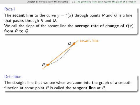
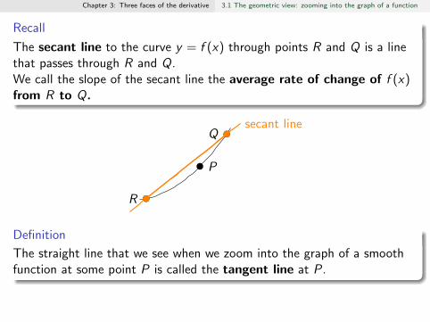
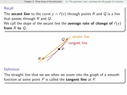
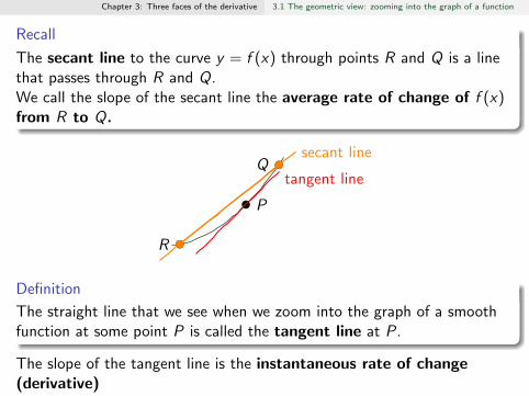
Recall
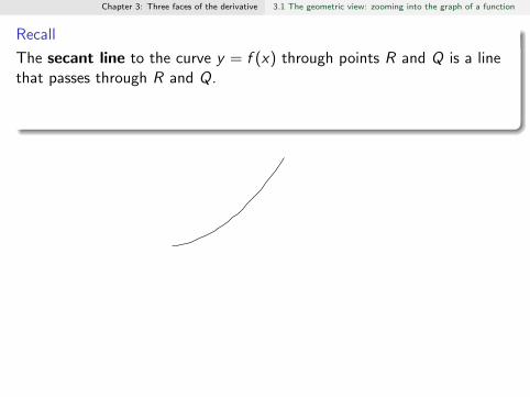
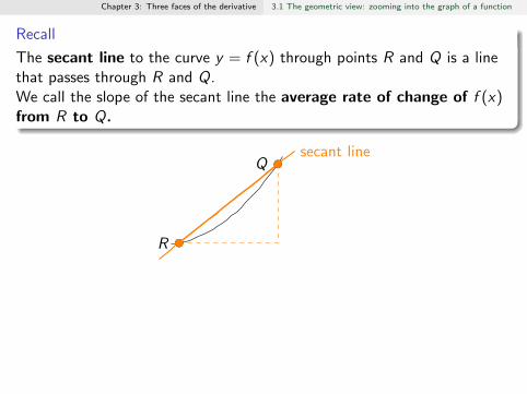
The secant line to the curve y = f (x) through points R and Q is a linethat passes through R and Q.
We call the slope of the secant line the average rate of change of f (x)from R to Q.
R
P
Qtangent line
secant line
Definition
The straight line that we see when we zoom into the graph of a smoothfunction at some point P is called the tangent line at P.
The slope of the tangent line is the instantaneous rate of change(derivative)of f (x) at P.

Chapter 3: Three faces of the derivative 3.1 The geometric view: zooming into the graph of a function
Recall
The secant line to the curve y = f (x) through points R and Q is a linethat passes through R and Q.
We call the slope of the secant line the average rate of change of f (x)from R to Q.
R
P
Q
tangent line
secant line
Definition
The straight line that we see when we zoom into the graph of a smoothfunction at some point P is called the tangent line at P.
The slope of the tangent line is the instantaneous rate of change(derivative)of f (x) at P.
Chapter 3: Three faces of the derivative 3.1 The geometric view: zooming into the graph of a function
Recall
The secant line to the curve y = f (x) through points R and Q is a linethat passes through R and Q.We call the slope of the secant line the average rate of change of f (x)from R to Q.
R
P
Qtangent line
secant line
Definition
The straight line that we see when we zoom into the graph of a smoothfunction at some point P is called the tangent line at P.
The slope of the tangent line is the instantaneous rate of change(derivative)of f (x) at P.

Chapter 3: Three faces of the derivative 3.1 The geometric view: zooming into the graph of a function
On the graph below, draw thesecant line to the curve throughpoints P and Q.
x
y
P
Q
On the graph below, draw thetangent line to the curve at point P.
x
y
P

Chapter 3: Three faces of the derivative 3.1 The geometric view: zooming into the graph of a function
On the graph below, draw thesecant line to the curve throughpoints P and Q.
x
y
P
Q
On the graph below, draw thetangent line to the curve at point P.
x
y
P

Chapter 3: Three faces of the derivative 3.1 The geometric view: zooming into the graph of a function
On the graph below, draw thesecant line to the curve throughpoints P and Q.
x
y
P
Q
On the graph below, draw thetangent line to the curve at point P.
x
y
P

Chapter 3: Three faces of the derivative 3.1 The geometric view: zooming into the graph of a function
Derivatives of Familiar Functions
1 The derivative of the function f (x) = Ax is:(a) 0(b) 1(c) A
X
(d) x(e) Ax
2 The derivative of the function f (x) = A is:(a) 0
X
(b) 1(c) A(d) x(e) Ax
3 The derivative of the function f (x) = A + x is:(a) 0(b) 1
X
(c) A(d) x(e) Ax

Chapter 3: Three faces of the derivative 3.1 The geometric view: zooming into the graph of a function
Derivatives of Familiar Functions
1 The derivative of the function f (x) = Ax is:(a) 0(b) 1(c) A X(d) x(e) Ax
2 The derivative of the function f (x) = A is:(a) 0 X(b) 1(c) A(d) x(e) Ax
3 The derivative of the function f (x) = A + x is:(a) 0(b) 1 X(c) A(d) x(e) Ax
Chapter 3: Three faces of the derivative 3.1 The geometric view: zooming into the graph of a function
ttime
ykm
from
hom
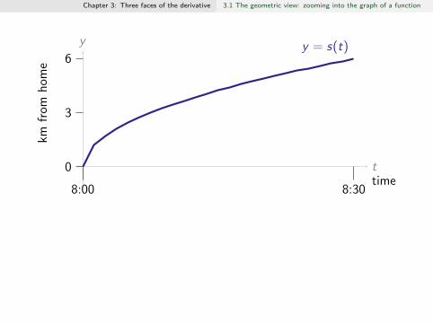
ey = s(t)
8:00 8:30
8:07
0
3
6
1/2 hour
6
8:25
A. secant line to y = s(t) from t = 8 : 00 to
B. slope of the secant line to y = s(t) from t = 8 : 00 to
C. tangent line to y = s(t) at
D. slope of the tangent line to y = s(t) at

Chapter 3: Three faces of the derivative 3.1 The geometric view: zooming into the graph of a function
ttime
ykm
from
hom
ey = s(t)
8:00 8:308:07
0
3
6
1/2 hour
6
8:25
A. secant line to y = s(t) from t = 8 : 00 to
B. slope of the secant line to y = s(t) from t = 8 : 00 to
C. tangent line to y = s(t) at
D. slope of the tangent line to y = s(t) at

Chapter 3: Three faces of the derivative 3.1 The geometric view: zooming into the graph of a function
ttime
ykm
from
hom
ey = s(t)
8:00 8:30
8:07
0
3
6
1/2 hour
6
8:25
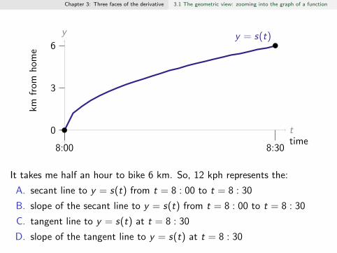
It takes me half an hour to bike 6 km. So, 12 kph represents the:
A. secant line to y = s(t) from t = 8 : 00 to t = 8 : 30
B. slope of the secant line to y = s(t) from t = 8 : 00 to t = 8 : 30
C. tangent line to y = s(t) at t = 8 : 30
D. slope of the tangent line to y = s(t) at t = 8 : 30
Chapter 3: Three faces of the derivative 3.1 The geometric view: zooming into the graph of a function
ttime
ykm
from
hom
ey = s(t)
8:00 8:30
8:07
0
3
6
1/2 hour
6
8:25
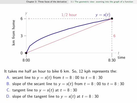
It takes me half an hour to bike 6 km. So, 12 kph represents the:
A. secant line to y = s(t) from t = 8 : 00 to t = 8 : 30
B. slope of the secant line to y = s(t) from t = 8 : 00 to t = 8 : 30
C. tangent line to y = s(t) at t = 8 : 30
D. slope of the tangent line to y = s(t) at t = 8 : 30

Chapter 3: Three faces of the derivative 3.1 The geometric view: zooming into the graph of a function
ttime
ykm
from
hom
ey = s(t)
8:00 8:30
8:07
0
3
6
1/2 hour
6
8:25
It takes me half an hour to bike 6 km. So, 12 kph represents the:
A. secant line to y = s(t) from t = 8 : 00 to t = 8 : 30
B. slope of the secant line to y = s(t) from t = 8 : 00 to t = 8 : 30
C. tangent line to y = s(t) at t = 8 : 30
D. slope of the tangent line to y = s(t) at t = 8 : 30

Chapter 3: Three faces of the derivative 3.1 The geometric view: zooming into the graph of a function
ttime
ykm
from
hom
ey = s(t)
8:00 8:30
8:07
0
3
61/2 hour
6
8:25
It takes me half an hour to bike 6 km. So, 12 kph represents the:
A. secant line to y = s(t) from t = 8 : 00 to t = 8 : 30
B. slope of the secant line to y = s(t) from t = 8 : 00 to t = 8 : 30
C. tangent line to y = s(t) at t = 8 : 30
D. slope of the tangent line to y = s(t) at t = 8 : 30

Chapter 3: Three faces of the derivative 3.1 The geometric view: zooming into the graph of a function
ttime
ykm
from
hom
ey = s(t)
8:00 8:30
8:07
0
3
6
1/2 hour
6
8:25
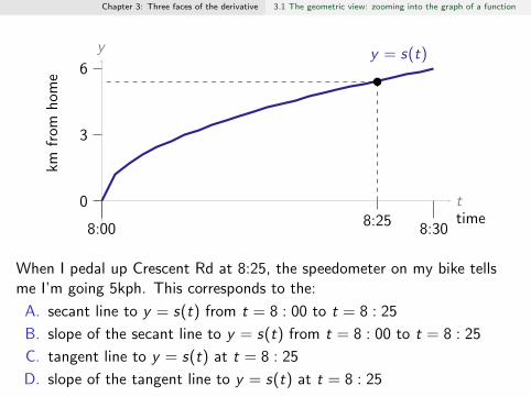
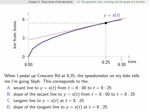
When I pedal up Crescent Rd at 8:25, the speedometer on my bike tellsme I’m going 5kph. This corresponds to the:
A. secant line to y = s(t) from t = 8 : 00 to t = 8 : 25
B. slope of the secant line to y = s(t) from t = 8 : 00 to t = 8 : 25
C. tangent line to y = s(t) at t = 8 : 25
D. slope of the tangent line to y = s(t) at t = 8 : 25
Chapter 3: Three faces of the derivative 3.1 The geometric view: zooming into the graph of a function
ttime
ykm
from
hom
ey = s(t)
8:00 8:30
8:07
0
3
6
1/2 hour
6
8:25
When I pedal up Crescent Rd at 8:25, the speedometer on my bike tellsme I’m going 5kph. This corresponds to the:
A. secant line to y = s(t) from t = 8 : 00 to t = 8 : 25
B. slope of the secant line to y = s(t) from t = 8 : 00 to t = 8 : 25
C. tangent line to y = s(t) at t = 8 : 25
D. slope of the tangent line to y = s(t) at t = 8 : 25

Chapter 3: Three faces of the derivative 3.1 The geometric view: zooming into the graph of a function
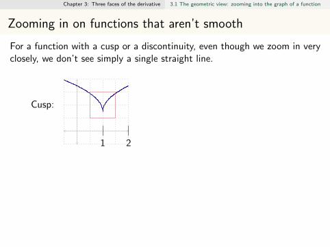
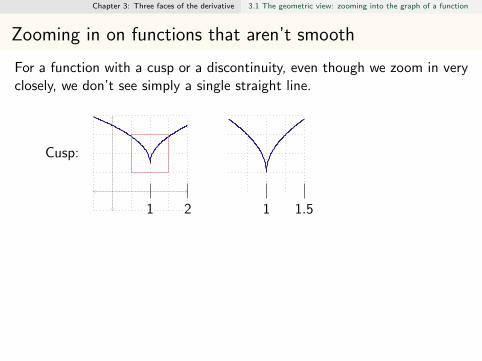
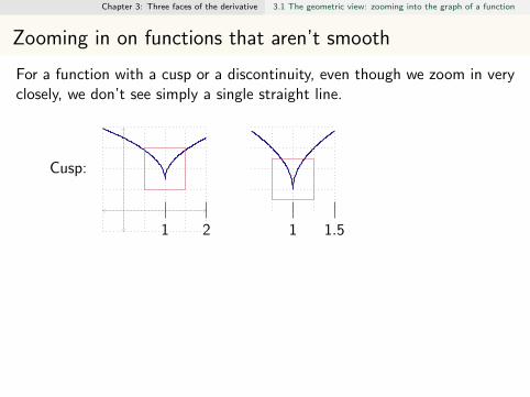
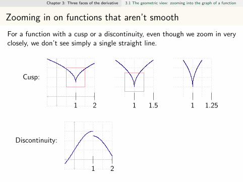
Zooming in on functions that aren’t smooth
For a function with a cusp or a discontinuity, even though we zoom in veryclosely, we don’t see simply a single straight line.
Cusp:
1 2
1 1.5 1 1.25
Discontinuity:
1 2
1 1.5 1 1.25
Chapter 3: Three faces of the derivative 3.1 The geometric view: zooming into the graph of a function
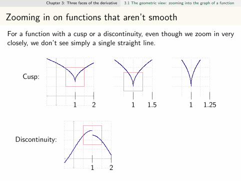
Zooming in on functions that aren’t smooth
For a function with a cusp or a discontinuity, even though we zoom in veryclosely, we don’t see simply a single straight line.
Cusp:
1 2 1 1.5
1 1.25
Discontinuity:
1 2
1 1.5 1 1.25
Chapter 3: Three faces of the derivative 3.1 The geometric view: zooming into the graph of a function
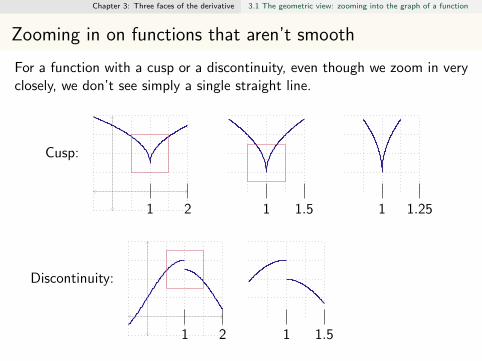
Zooming in on functions that aren’t smooth
For a function with a cusp or a discontinuity, even though we zoom in veryclosely, we don’t see simply a single straight line.
Cusp:
1 2 1 1.5
1 1.25
Discontinuity:
1 2
1 1.5 1 1.25

Chapter 3: Three faces of the derivative 3.1 The geometric view: zooming into the graph of a function
Zooming in on functions that aren’t smooth
For a function with a cusp or a discontinuity, even though we zoom in veryclosely, we don’t see simply a single straight line.
Cusp:
1 2 1 1.5 1 1.25
Discontinuity:
1 2
1 1.5 1 1.25
Chapter 3: Three faces of the derivative 3.1 The geometric view: zooming into the graph of a function
Zooming in on functions that aren’t smooth
For a function with a cusp or a discontinuity, even though we zoom in veryclosely, we don’t see simply a single straight line.
Cusp:
1 2 1 1.5 1 1.25
Discontinuity:
1 2 1 1.5
1 1.25

Chapter 3: Three faces of the derivative 3.1 The geometric view: zooming into the graph of a function
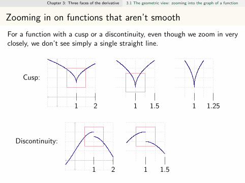
Zooming in on functions that aren’t smooth
For a function with a cusp or a discontinuity, even though we zoom in veryclosely, we don’t see simply a single straight line.
Cusp:
1 2 1 1.5 1 1.25
Discontinuity:
1 2 1 1.5 1 1.25

Chapter 3: Three faces of the derivative 3.1 The geometric view: zooming into the graph of a function
Zooming in on functions that aren’t smooth
For a function with a cusp or a discontinuity, even though we zoom in veryclosely, we don’t see simply a single straight line.
Cusp:
1 2 1 1.5 1 1.25
Discontinuity:
1 2 1 1.5 1 1.25
Photo credit: Pixabay

Chapter 3: Three faces of the derivative 3.1 The geometric view: zooming into the graph of a function
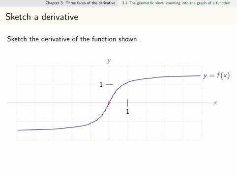
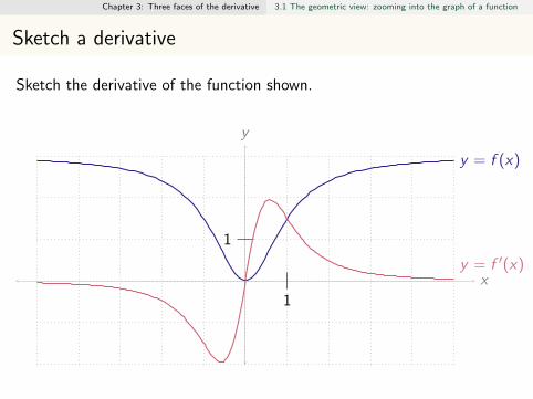
Sketch a derivative
Sketch the derivative of the function shown.
x
y
y = f (x)
1
1
•
2
•
14
•
14 ≈ 0≈ 0
y = f ′(x)
Chapter 3: Three faces of the derivative 3.1 The geometric view: zooming into the graph of a function
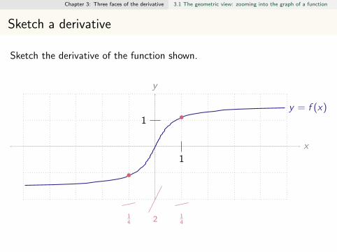
Sketch a derivative
Sketch the derivative of the function shown.
x
y
y = f (x)
1
1
•
2
•
14
•
14 ≈ 0≈ 0
y = f ′(x)

Chapter 3: Three faces of the derivative 3.1 The geometric view: zooming into the graph of a function
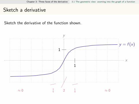
Sketch a derivative
Sketch the derivative of the function shown.
x
y
y = f (x)
1
1
•
2
•
14
•
14 ≈ 0≈ 0
y = f ′(x)

Chapter 3: Three faces of the derivative 3.1 The geometric view: zooming into the graph of a function
Sketch a derivative
Sketch the derivative of the function shown.
x
y
y = f (x)
1
1
•
2
•
14
•
14 ≈ 0≈ 0
y = f ′(x)

Chapter 3: Three faces of the derivative 3.1 The geometric view: zooming into the graph of a function
Sketch a derivative
Sketch the derivative of the function shown.
x
y
y = f (x)
1
1
•
2
•
14
•
14 ≈ 0≈ 0
y = f ′(x)

Chapter 3: Three faces of the derivative 3.1 The geometric view: zooming into the graph of a function
Sketch a derivative
Sketch the derivative of the function shown.
x
y
y = f (x)
1
1
•
2
•
14
•
14 ≈ 0≈ 0
y = f ′(x)
Chapter 3: Three faces of the derivative 3.1 The geometric view: zooming into the graph of a function
Sketch a derivative
Sketch the derivative of the function shown.
x
y
y = f (x)
1
1
•
2
•
14
•
14
≈ 0≈ 0
y = f ′(x)
Chapter 3: Three faces of the derivative 3.1 The geometric view: zooming into the graph of a function
Sketch a derivative
Sketch the derivative of the function shown.
x
y
y = f (x)
1
1
•
2
•
14
•
14 ≈ 0≈ 0
y = f ′(x)

Chapter 3: Three faces of the derivative 3.1 The geometric view: zooming into the graph of a function
Sketch a derivative
Sketch the derivative of the function shown.
x
y
y = f (x)
1
1
•
2
•
14
•
14 ≈ 0≈ 0
y = f ′(x)
Chapter 3: Three faces of the derivative 3.1 The geometric view: zooming into the graph of a function
Sketch a derivative
Sketch the derivative of the function shown.
x
y
y = f (x)
1
1
y = f ′(x)
Chapter 3: Three faces of the derivative 3.1 The geometric view: zooming into the graph of a function
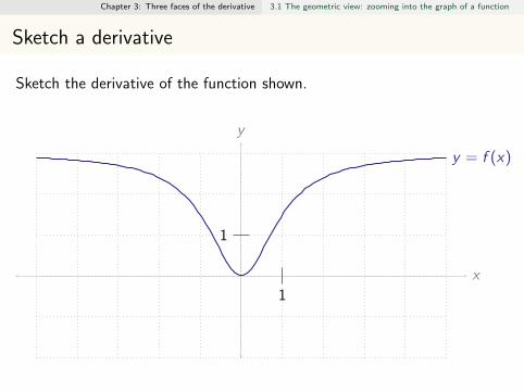
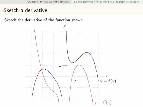
Sketch a derivative
Sketch the derivative of the function shown.
x
y
y = f (x)
1
1
y = f ′(x)

Chapter 3: Three faces of the derivative 3.1 The geometric view: zooming into the graph of a function
Sketch a derivative
Sketch the derivative of the function shown.
x
y
y = f (x)1
1
y = f ′(x)
Chapter 3: Three faces of the derivative 3.1 The geometric view: zooming into the graph of a function
Sketch a derivative
Sketch the derivative of the function shown.
x
y
y = f (x)1
1
y = f ′(x)

Chapter 3: Three faces of the derivative 3.1 The geometric view: zooming into the graph of a function
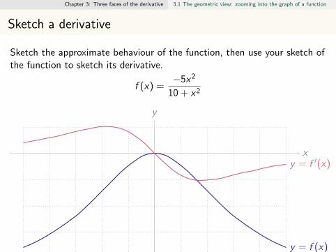
Sketch a derivative
Sketch the approximate behaviour of the function, then use your sketch ofthe function to sketch its derivative.
f (x) =−5x2
10 + x2
x
y
y = f (x)
y = f ′(x)

Chapter 3: Three faces of the derivative 3.1 The geometric view: zooming into the graph of a function
Sketch a derivative
Sketch the approximate behaviour of the function, then use your sketch ofthe function to sketch its derivative.
f (x) =−5x2
10 + x2
x
y
y = f (x)
y = f ′(x)
Chapter 3: Three faces of the derivative 3.1 The geometric view: zooming into the graph of a function
Sketch a derivative
Sketch the approximate behaviour of the function, then use your sketch ofthe function to sketch its derivative.
f (x) =−5x2
10 + x2
x
y
y = f (x)
y = f ′(x)

Chapter 3: Three faces of the derivative 3.1 The geometric view: zooming into the graph of a function
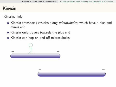
Kinesin
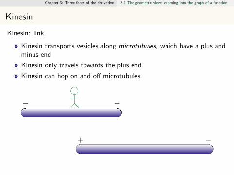
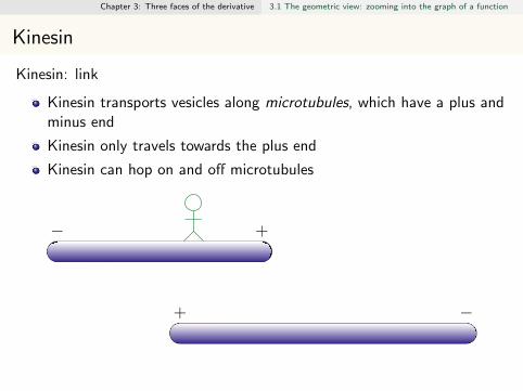
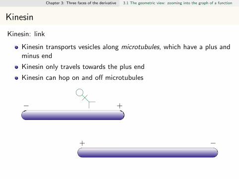
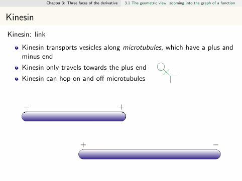
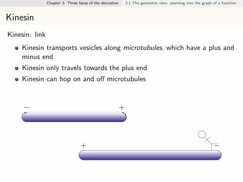
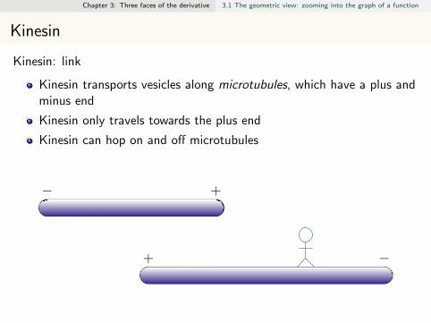
Kinesin: link
Kinesin transports vesicles along microtubules, which have a plus andminus end
Kinesin only travels towards the plus end
Kinesin can hop on and off microtubules
+−
−+
More explanation of Kinesin’s walking: link

Chapter 3: Three faces of the derivative 3.1 The geometric view: zooming into the graph of a function
Kinesin
Kinesin: link
Kinesin transports vesicles along microtubules, which have a plus andminus end
Kinesin only travels towards the plus end
Kinesin can hop on and off microtubules
+−
−+
More explanation of Kinesin’s walking: link

Chapter 3: Three faces of the derivative 3.1 The geometric view: zooming into the graph of a function
Kinesin
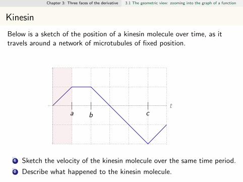
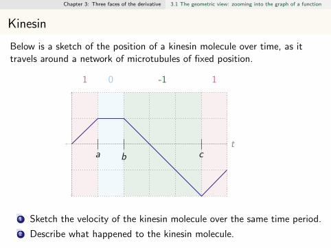
Below is a sketch of the position of a kinesin molecule over time, as ittravels around a network of microtubules of fixed position.
ta b c
1 Sketch the velocity of the kinesin molecule over the same time period.
2 Describe what happened to the kinesin molecule.
Chapter 3: Three faces of the derivative 3.1 The geometric view: zooming into the graph of a function
Kinesin
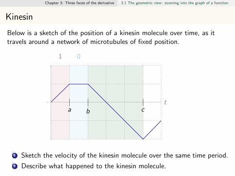
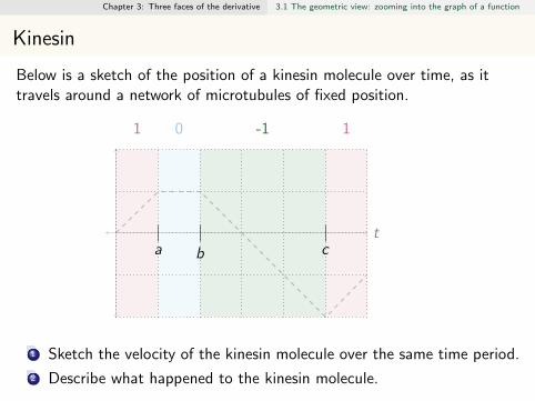
Below is a sketch of the position of a kinesin molecule over time, as ittravels around a network of microtubules of fixed position.
ta b c
1 0 -1 1
velocity
1 Sketch the velocity of the kinesin molecule over the same time period.
2 Describe what happened to the kinesin molecule.

Chapter 3: Three faces of the derivative 3.1 The geometric view: zooming into the graph of a function
Kinesin
Below is a sketch of the position of a kinesin molecule over time, as ittravels around a network of microtubules of fixed position.
ta b c
1
0 -1 1
velocity
1 Sketch the velocity of the kinesin molecule over the same time period.
2 Describe what happened to the kinesin molecule.

Chapter 3: Three faces of the derivative 3.1 The geometric view: zooming into the graph of a function
Kinesin
Below is a sketch of the position of a kinesin molecule over time, as ittravels around a network of microtubules of fixed position.
ta b c
1 0
-1 1
velocity
1 Sketch the velocity of the kinesin molecule over the same time period.
2 Describe what happened to the kinesin molecule.

Chapter 3: Three faces of the derivative 3.1 The geometric view: zooming into the graph of a function
Kinesin
Below is a sketch of the position of a kinesin molecule over time, as ittravels around a network of microtubules of fixed position.
ta b c
1 0 -1
1
velocity
1 Sketch the velocity of the kinesin molecule over the same time period.
2 Describe what happened to the kinesin molecule.
Chapter 3: Three faces of the derivative 3.1 The geometric view: zooming into the graph of a function
Kinesin
Below is a sketch of the position of a kinesin molecule over time, as ittravels around a network of microtubules of fixed position.
ta b c
1 0 -1 1
velocity
1 Sketch the velocity of the kinesin molecule over the same time period.
2 Describe what happened to the kinesin molecule.
Chapter 3: Three faces of the derivative 3.1 The geometric view: zooming into the graph of a function
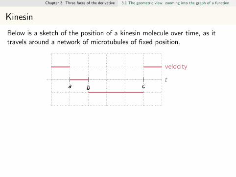
Kinesin
Below is a sketch of the position of a kinesin molecule over time, as ittravels around a network of microtubules of fixed position.
ta b c
velocity
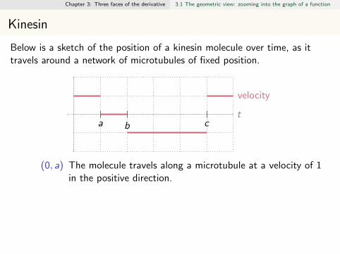
(0, a) The molecule travels along a microtubule at a velocity of 1in the positive direction.
(a, b) Then, it falls off or gets stuck.
(b, c) Then it travels on along a mictorubule with the oppositeorientation, so it moves in the negative direction.
t > c Finally, it hops onto another microtubule (possibly the sameas the first) and travels in the positive direction.
Chapter 3: Three faces of the derivative 3.1 The geometric view: zooming into the graph of a function
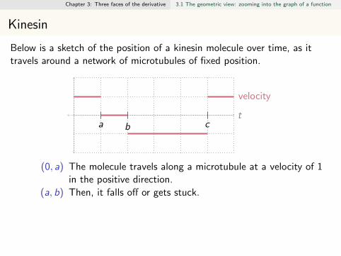
Kinesin
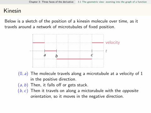
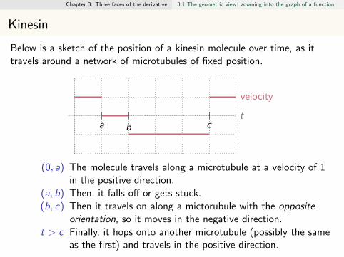
Below is a sketch of the position of a kinesin molecule over time, as ittravels around a network of microtubules of fixed position.
ta b c
velocity
(0, a) The molecule travels along a microtubule at a velocity of 1in the positive direction.
(a, b) Then, it falls off or gets stuck.
(b, c) Then it travels on along a mictorubule with the oppositeorientation, so it moves in the negative direction.
t > c Finally, it hops onto another microtubule (possibly the sameas the first) and travels in the positive direction.
Chapter 3: Three faces of the derivative 3.1 The geometric view: zooming into the graph of a function
Kinesin
Below is a sketch of the position of a kinesin molecule over time, as ittravels around a network of microtubules of fixed position.
ta b c
velocity
(0, a) The molecule travels along a microtubule at a velocity of 1in the positive direction.
(a, b) Then, it falls off or gets stuck.
(b, c) Then it travels on along a mictorubule with the oppositeorientation, so it moves in the negative direction.
t > c Finally, it hops onto another microtubule (possibly the sameas the first) and travels in the positive direction.
Chapter 3: Three faces of the derivative 3.2 The analytic view: calculating the derivative
Overview
Explain the definition of a continuous function.
Identify functions with various types of discontinuities.
Evaluate simple limits of rational functions.
Calculate the derivative of a simple function using the definition ofthe derivative
Chapter 3: Three faces of the derivative 3.2 The analytic view: calculating the derivative
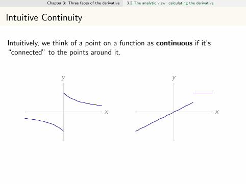
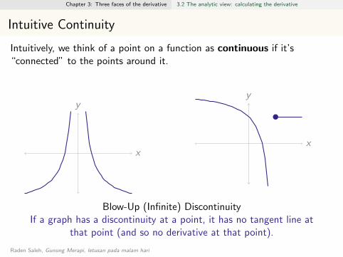
Intuitive Continuity
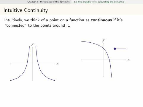
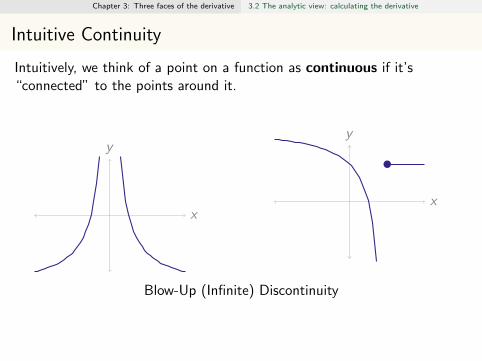
Intuitively, we think of a point on a function as continuous if it’s“connected” to the points around it.
x
y
x
y
Jump Discontinuity

Chapter 3: Three faces of the derivative 3.2 The analytic view: calculating the derivative
Intuitive Continuity
Intuitively, we think of a point on a function as continuous if it’s“connected” to the points around it.
x
y
x
y
Jump Discontinuity
Chapter 3: Three faces of the derivative 3.2 The analytic view: calculating the derivative
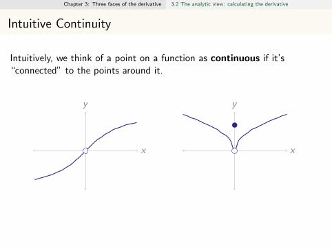
Intuitive Continuity
Intuitively, we think of a point on a function as continuous if it’s“connected” to the points around it.
x
y
x
y
Removable Discontinuity

Chapter 3: Three faces of the derivative 3.2 The analytic view: calculating the derivative
Intuitive Continuity
Intuitively, we think of a point on a function as continuous if it’s“connected” to the points around it.
x
y
x
y
Removable Discontinuity
Chapter 3: Three faces of the derivative 3.2 The analytic view: calculating the derivative
Intuitive Continuity
Intuitively, we think of a point on a function as continuous if it’s“connected” to the points around it.
x
y
x
y
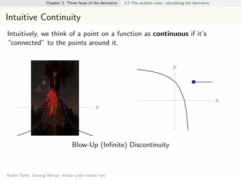
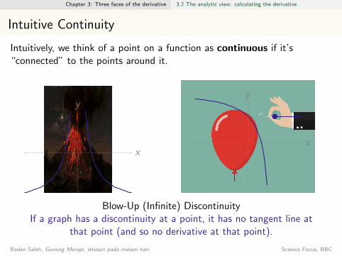
Blow-Up (Infinite) DiscontinuityIf a graph has a discontinuity at a point, it has no tangent line at
that point (and so no derivative at that point).
Raden Saleh, Gunung Merapi, letusan pada malam hari Science Focus, BBC
Chapter 3: Three faces of the derivative 3.2 The analytic view: calculating the derivative
Intuitive Continuity
Intuitively, we think of a point on a function as continuous if it’s“connected” to the points around it.
x
y
x
y
Blow-Up (Infinite) Discontinuity
If a graph has a discontinuity at a point, it has no tangent line atthat point (and so no derivative at that point).
Raden Saleh, Gunung Merapi, letusan pada malam hari
Science Focus, BBC

Chapter 3: Three faces of the derivative 3.2 The analytic view: calculating the derivative
Intuitive Continuity
Intuitively, we think of a point on a function as continuous if it’s“connected” to the points around it.
x
y
x
y
Blow-Up (Infinite) Discontinuity
If a graph has a discontinuity at a point, it has no tangent line atthat point (and so no derivative at that point).
Raden Saleh, Gunung Merapi, letusan pada malam hari Science Focus, BBC
Chapter 3: Three faces of the derivative 3.2 The analytic view: calculating the derivative
Intuitive Continuity
Intuitively, we think of a point on a function as continuous if it’s“connected” to the points around it.
x
y
x
y
Blow-Up (Infinite) DiscontinuityIf a graph has a discontinuity at a point, it has no tangent line at
that point (and so no derivative at that point).
Raden Saleh, Gunung Merapi, letusan pada malam hari Science Focus, BBC
Chapter 3: Three faces of the derivative 3.2 The analytic view: calculating the derivative
Intuitive Continuity
Intuitively, we think of a point on a function as continuous if it’s“connected” to the points around it.
x
y
x
y
Blow-Up (Infinite) DiscontinuityIf a graph has a discontinuity at a point, it has no tangent line at
that point (and so no derivative at that point).
Raden Saleh, Gunung Merapi, letusan pada malam hari
Science Focus, BBC
Chapter 3: Three faces of the derivative 3.2 The analytic view: calculating the derivative
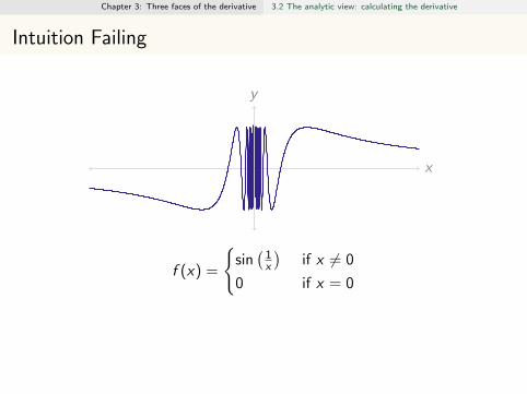
Intuition Failing
x
y
f (x) =
{sin(1x
)if x 6= 0
0 if x = 0

Chapter 3: Three faces of the derivative 3.2 The analytic view: calculating the derivative
Intuition Failing
x
y
f (x) =
{sin(1x
)if x 6= 0
1 if x = 0
Chapter 3: Three faces of the derivative 3.2 The analytic view: calculating the derivative
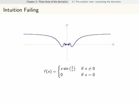
Intuition Failing
x
y
•
f (x) =
{x sin
(1x
)if x 6= 0
0 if x = 0
Chapter 3: Three faces of the derivative 3.2 The analytic view: calculating the derivative
Intuition Failing
x
y•
•
•
•
•
•
•
•
•
•
•
•
•
•
•
•
•
•
•
•
•
•
•
•
•
•
•
•
•
•
•
•
•
•
•
•
•
•
•
•
•
•
•
•
•
•
•
•
•
•
•
•
•
•
•
•
•
•
•
•
•
••••••••••••••••••••••••••••
••••••••••••
•
•
•
•
•
•
•
•
•
•
•
•
•
•
•
•
•
•
•
•
•
•
•
•
•
•
•
•
•
•
•
•
•
•
•
•
•
•
•
•
•
•
•
•
•
•
•
•
•
•
•
•
•
•
•
•
•
•
•
•
•
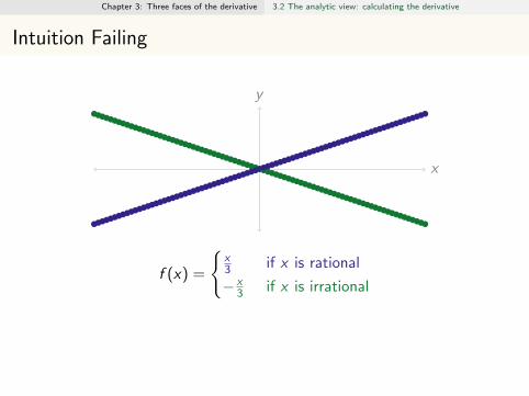
f (x) =
{x3 if x is rational
− x3 if x is irrational
Chapter 3: Three faces of the derivative 3.2 The analytic view: calculating the derivative
A More Rigorous Definition
Definition
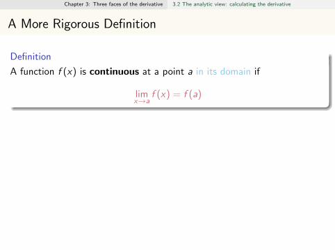
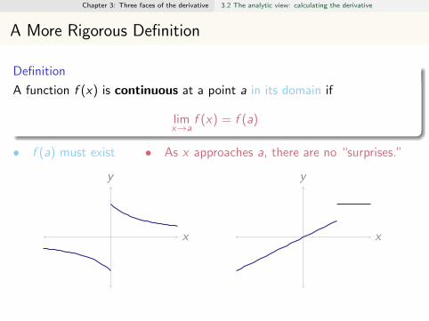
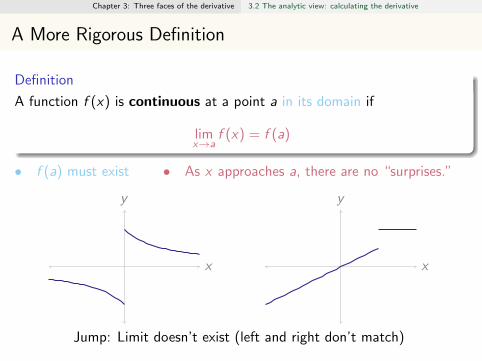
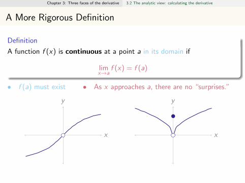
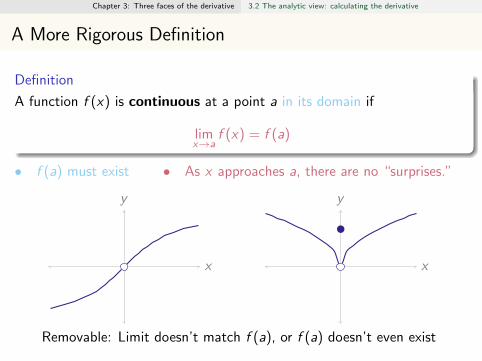
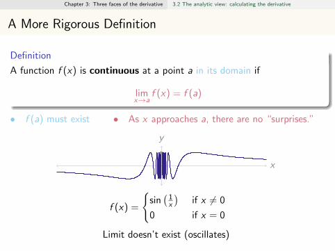
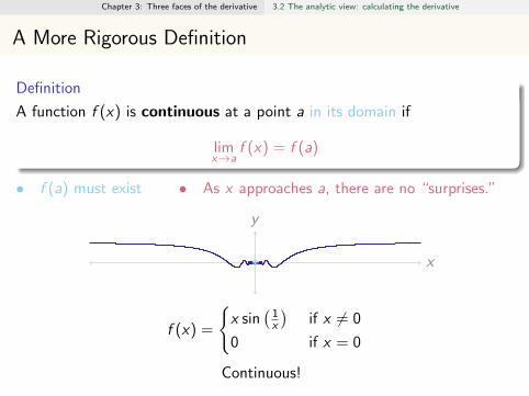
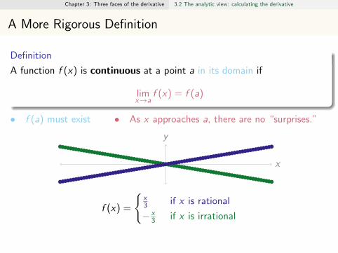
A function f (x) is continuous at a point a in its domain if
limx→a
f (x) = f (a)
• f (a) must exist • As x approaches a, there are no “surprises.”

Chapter 3: Three faces of the derivative 3.2 The analytic view: calculating the derivative
A More Rigorous Definition
Definition
A function f (x) is continuous at a point a in its domain if
limx→a
f (x) = f (a)
• f (a) must exist • As x approaches a, there are no “surprises.”
Chapter 3: Three faces of the derivative 3.2 The analytic view: calculating the derivative
A More Rigorous Definition
Definition
A function f (x) is continuous at a point a in its domain if
limx→a
f (x) = f (a)
• f (a) must exist • As x approaches a, there are no “surprises.”
x
y
x
y
Jump: Limit doesn’t exist (left and right don’t match)
Chapter 3: Three faces of the derivative 3.2 The analytic view: calculating the derivative
A More Rigorous Definition
Definition
A function f (x) is continuous at a point a in its domain if
limx→a
f (x) = f (a)
• f (a) must exist • As x approaches a, there are no “surprises.”
x
y
x
y
Removable: Limit doesn’t match f (a), or f (a) doesn’t even exist

Chapter 3: Three faces of the derivative 3.2 The analytic view: calculating the derivative
A More Rigorous Definition
Definition
A function f (x) is continuous at a point a in its domain if
limx→a
f (x) = f (a)
• f (a) must exist • As x approaches a, there are no “surprises.”
x
y
x
y
Blow-up: Limit doesn’t exist.

Chapter 3: Three faces of the derivative 3.2 The analytic view: calculating the derivative
A More Rigorous Definition
Definition
A function f (x) is continuous at a point a in its domain if
limx→a
f (x) = f (a)
• f (a) must exist • As x approaches a, there are no “surprises.”
x
y
f (x) =
{sin(1x
)if x 6= 0
0 if x = 0
Limit doesn’t exist (oscillates)

Chapter 3: Three faces of the derivative 3.2 The analytic view: calculating the derivative
A More Rigorous Definition
Definition
A function f (x) is continuous at a point a in its domain if
limx→a
f (x) = f (a)
• f (a) must exist • As x approaches a, there are no “surprises.”
x
y
•
f (x) =
{x sin
(1x
)if x 6= 0
0 if x = 0
Continuous!
Chapter 3: Three faces of the derivative 3.2 The analytic view: calculating the derivative
A More Rigorous Definition
Definition
A function f (x) is continuous at a point a in its domain if
limx→a
f (x) = f (a)
• f (a) must exist • As x approaches a, there are no “surprises.”
x
y•
•
•
•
•
•
•
•
•
•
•
•
•
•
•
•
•
•
•
•
•
•
•
•
•
•
•
•
•
•
•
•
•
•
•
•
•
•
•
•
•
••••••••••••••••••••••••••••••••••••••••••••••••••••••••
••••••••••••••••••••••••
•
•
•
•
•
•
•
•
•
•
•
•
•
•
•
•
•
•
•
•
•
•
•
•
•
•
•
•
•
•
•
•
•
•
•
•
•
•
•
•
•
f (x) =
{x3 if x is rational
− x3 if x is irrational
Continuous at x = 0; discontinuous elsewhere.(A more rigorous limit definition is helpful here.)
Chapter 3: Three faces of the derivative 3.2 The analytic view: calculating the derivative
Continuity Proofs
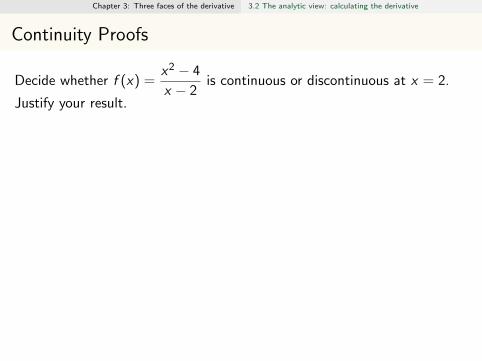
Decide whether f (x) =x2 − 4
x − 2is continuous or discontinuous at x = 2.
Justify your result.
It is discontinuous, because 2 is not in the domain of f (x). That is, f (2)does not exist.Example 1:
For which value(s) of a is f (x) =
x2 − 4
x − 2if x 6= 2
a if x = 2continuous at x = 2?
Prove your result.Only for a = 4.If x 6= 2, then f (x) = x2−4
x−2 = (x+2)(x−2)x−2 = x + 2. So,
limx→2
f (x) = limx→2
x + 2 = 4.
In order for f (x) to be continuous at x = 2, we need:
limx→2
f (x) = f (2)
That is, we need 4=a.

Chapter 3: Three faces of the derivative 3.2 The analytic view: calculating the derivative
Continuity Proofs
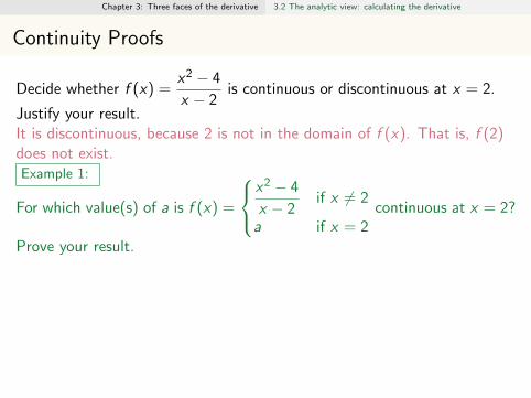
Decide whether f (x) =x2 − 4
x − 2is continuous or discontinuous at x = 2.
Justify your result.It is discontinuous, because 2 is not in the domain of f (x). That is, f (2)does not exist.
Example 1:
For which value(s) of a is f (x) =
x2 − 4
x − 2if x 6= 2
a if x = 2continuous at x = 2?
Prove your result.Only for a = 4.If x 6= 2, then f (x) = x2−4
x−2 = (x+2)(x−2)x−2 = x + 2. So,
limx→2
f (x) = limx→2
x + 2 = 4.
In order for f (x) to be continuous at x = 2, we need:
limx→2
f (x) = f (2)
That is, we need 4=a.
Chapter 3: Three faces of the derivative 3.2 The analytic view: calculating the derivative
Continuity Proofs
Decide whether f (x) =x2 − 4
x − 2is continuous or discontinuous at x = 2.
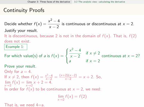
Justify your result.It is discontinuous, because 2 is not in the domain of f (x). That is, f (2)does not exist.Example 1:
For which value(s) of a is f (x) =
x2 − 4
x − 2if x 6= 2
a if x = 2continuous at x = 2?
Prove your result.
Only for a = 4.If x 6= 2, then f (x) = x2−4
x−2 = (x+2)(x−2)x−2 = x + 2. So,
limx→2
f (x) = limx→2
x + 2 = 4.
In order for f (x) to be continuous at x = 2, we need:
limx→2
f (x) = f (2)
That is, we need 4=a.
Chapter 3: Three faces of the derivative 3.2 The analytic view: calculating the derivative
Continuity Proofs
Decide whether f (x) =x2 − 4
x − 2is continuous or discontinuous at x = 2.
Justify your result.It is discontinuous, because 2 is not in the domain of f (x). That is, f (2)does not exist.Example 1:
For which value(s) of a is f (x) =
x2 − 4
x − 2if x 6= 2
a if x = 2continuous at x = 2?
Prove your result.Only for a = 4.If x 6= 2, then f (x) = x2−4
x−2 = (x+2)(x−2)x−2 = x + 2. So,
limx→2
f (x) = limx→2
x + 2 = 4.
In order for f (x) to be continuous at x = 2, we need:
limx→2
f (x) = f (2)
That is, we need 4=a.

Chapter 3: Three faces of the derivative 3.2 The analytic view: calculating the derivative
Rational Functions with Holes
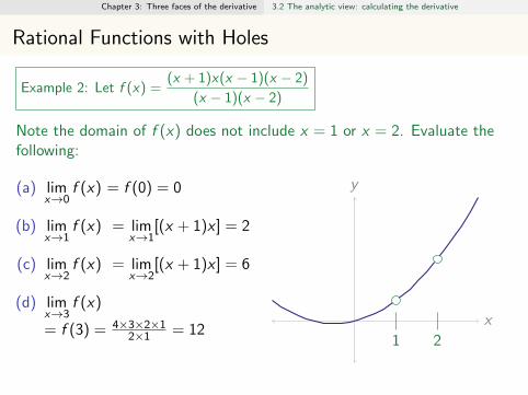
Example 2: Let f (x) =(x + 1)x(x − 1)(x − 2)
(x − 1)(x − 2)
Note the domain of f (x) does not include x = 1 or x = 2. Evaluate thefollowing:
(a) limx→0
f (x)
= f (0) = 0
(b) limx→1
f (x)
= limx→1
[(x + 1)x ] = 2
(c) limx→2
f (x)
= limx→2
[(x + 1)x ] = 6
(d) limx→3
f (x)
= f (3) = 4×3×2×12×1 = 12
x
y
1 2

Chapter 3: Three faces of the derivative 3.2 The analytic view: calculating the derivative
Rational Functions with Holes
Example 2: Let f (x) =(x + 1)x(x − 1)(x − 2)
(x − 1)(x − 2)
Note the domain of f (x) does not include x = 1 or x = 2. Evaluate thefollowing:
(a) limx→0
f (x)
= f (0) = 0
(b) limx→1
f (x)
= limx→1
[(x + 1)x ] = 2
(c) limx→2
f (x)
= limx→2
[(x + 1)x ] = 6
(d) limx→3
f (x)
= f (3) = 4×3×2×12×1 = 12
x
y
1 2
Chapter 3: Three faces of the derivative 3.2 The analytic view: calculating the derivative
Rational Functions with Holes
Example 2: Let f (x) =(x + 1)x(x − 1)(x − 2)
(x − 1)(x − 2)
Note the domain of f (x) does not include x = 1 or x = 2. Evaluate thefollowing:
(a) limx→0
f (x) = f (0) = 0
(b) limx→1
f (x) = limx→1
[(x + 1)x ] = 2
(c) limx→2
f (x) = limx→2
[(x + 1)x ] = 6
(d) limx→3
f (x)
= f (3) = 4×3×2×12×1 = 12
x
y
1 2

Chapter 3: Three faces of the derivative 3.2 The analytic view: calculating the derivative
Using limits to evaluate derivatives
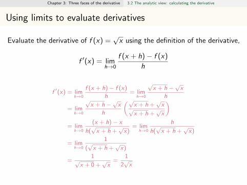
Evaluate the derivative of f (x) =√x using the definition of the derivative,
f ′(x) = limh→0
f (x + h)− f (x)
h
f ′(x) = limh→0
f (x + h)− f (x)
h= lim
h→0
√x + h −
√x
h
= limh→0
√x + h −
√x
h
(√x + h +
√x√
x + h +√x
)= lim
h→0
(x + h)− x
h(√x + h +
√x)
= limh→0
h
h(√x + h +
√x)
= limh→0
1
(√x + h +
√x)
=1√
x + 0 +√x=
1
2√x
Chapter 3: Three faces of the derivative 3.2 The analytic view: calculating the derivative
Using limits to evaluate derivatives
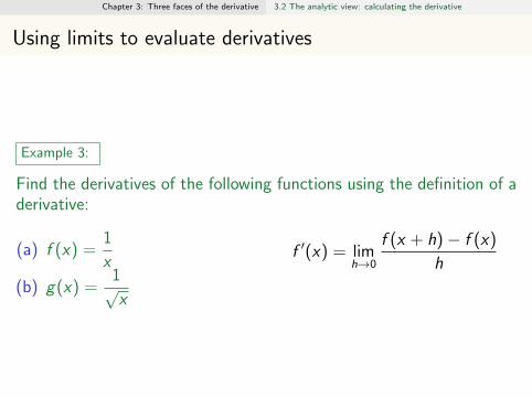
Example 3:
Find the derivatives of the following functions using the definition of aderivative:
(a) f (x) =1
x
(b) g(x) =1√x
f ′(x) = limh→0
f (x + h)− f (x)
h

Chapter 3: Three faces of the derivative 3.2 The analytic view: calculating the derivative
Using limits to evaluate derivatives
Example 3:
Find the derivatives of the following functions using the definition of aderivative:
(a) f (x) =1
x
(b) g(x) =1√x
f ′(x) = limh→0
f (x + h)− f (x)
h
f ′(x) = limh→0
f (x + h)− f (x)
h= lim
h→0
1x+h− 1
x
h= lim
h→0
xx(x+h)
− x+hx(x+h)
h
= limh→0
x − (x + h)
x(x + h)(h)= lim
h→0
−hx(x + h)(h)
= limh→0
−1
x(x + h)
=−1
x(x + 0)= − 1
x2
Chapter 3: Three faces of the derivative 3.2 The analytic view: calculating the derivative
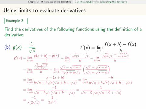
Using limits to evaluate derivatives
Example 3:
Find the derivatives of the following functions using the definition of aderivative:
(b) g(x) =1√x
f ′(x) = limh→0
f (x + h)− f (x)
h
g ′(x) = limh→0
g(x + h)− g(x)
h= lim
h→0
1√x+h− 1√
x
h= lim
h→0
√x√
x+h√x−
√x+h√
x+h√x
h
= limh→0
√x−√x+h√
x+h√
x
h= lim
h→0
√x −√x + h
h√x + h
√x
(√x +√x + h
√x +√x + h
)= lim
x→0
x − (x + h)
h√x + h
√x(√x + h +
√x)
= limx→0
−hh√x + h
√x(√x + h +
√x)
= limx→0
−1√x + h
√x(√x + h +
√x)
=1√
x + 0√x(√x + 0 +
√x)
=−1
x(2√x)
= − 1
2x3/2
Chapter 3: Three faces of the derivative 3.2 The analytic view: calculating the derivative
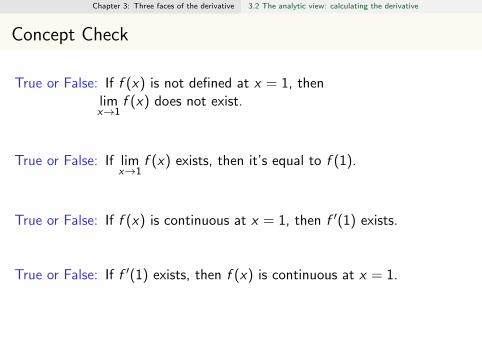
Concept Check
True or False: If f (x) is not defined at x = 1, thenlimx→1
f (x) does not exist.
True or False: If limx→1
f (x) exists, then it’s equal to f (1).
True or False: If f (x) is continuous at x = 1, then f ′(1) exists.
True or False: If f ′(1) exists, then f (x) is continuous at x = 1.
Chapter 3: Three faces of the derivative 3.2 The analytic view: calculating the derivative
Concept Check
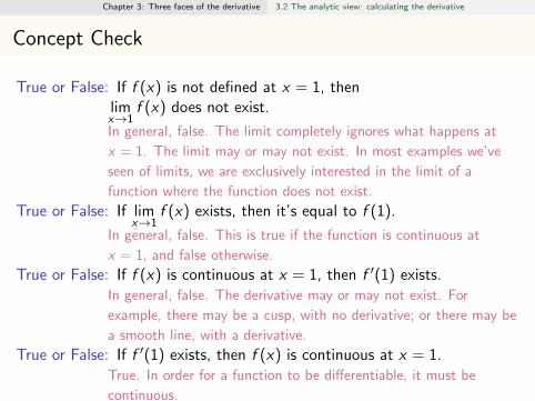
True or False: If f (x) is not defined at x = 1, thenlimx→1
f (x) does not exist.
In general, false. The limit completely ignores what happens at
x = 1. The limit may or may not exist. In most examples we’ve
seen of limits, we are exclusively interested in the limit of a
function where the function does not exist.
True or False: If limx→1
f (x) exists, then it’s equal to f (1).
In general, false. This is true if the function is continuous at
x = 1, and false otherwise.
True or False: If f (x) is continuous at x = 1, then f ′(1) exists.In general, false. The derivative may or may not exist. For
example, there may be a cusp, with no derivative; or there may be
a smooth line, with a derivative.
True or False: If f ′(1) exists, then f (x) is continuous at x = 1.True. In order for a function to be differentiable, it must be
continuous.

Chapter 3: Three faces of the derivative 3.2 The analytic view: calculating the derivative
Using Graphs
Example 4: Approximate limx→0
sin x
xusing the graph below.
x
y
1
limx→0
sin x
x= 1
Chapter 3: Three faces of the derivative 3.2 The analytic view: calculating the derivative
Using Graphs
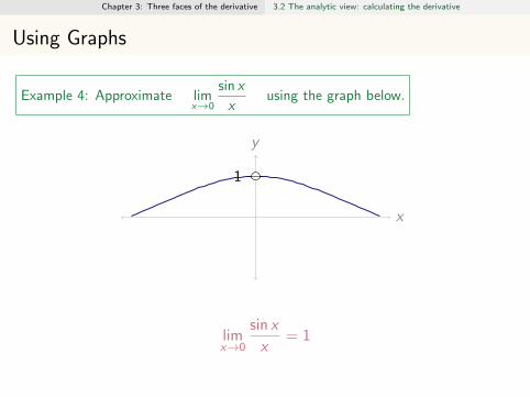
Example 4: Approximate limx→0
sin x
xusing the graph below.
x
y
1
limx→0
sin x
x= 1

Chapter 3: Three faces of the derivative 3.3 The computational view: software to the rescue!
Overview
1 Use software to numerically compute an approximation to thederivative.
2 Explain that the approximation replaces a (true) tangent line with an(approximating) secant line.
3 Explain using words how the derivative shape is connected with theshape of the original function.
.
Chapter 3: Three faces of the derivative 3.3 The computational view: software to the rescue!
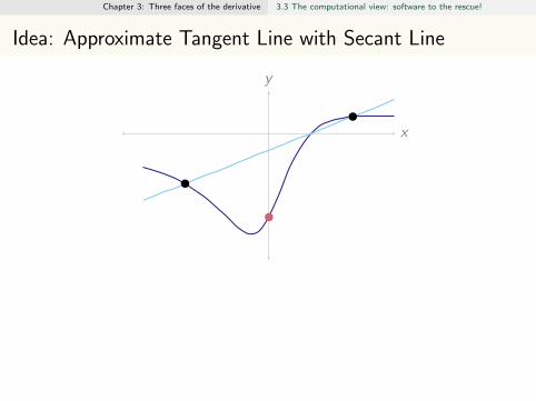
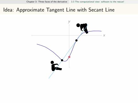
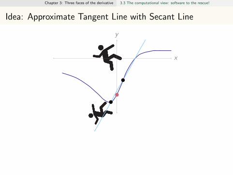
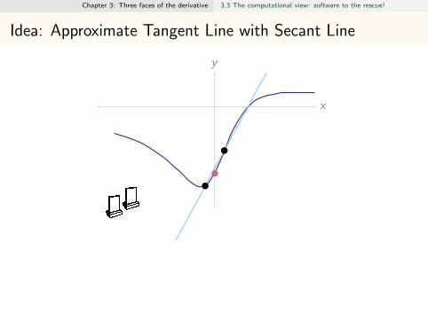
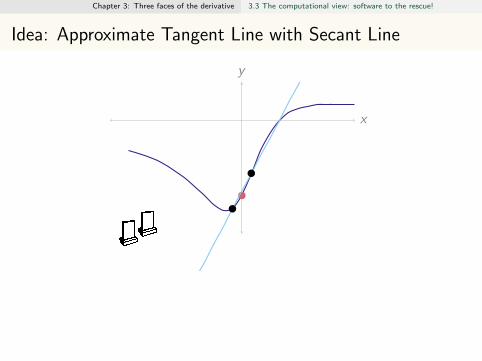
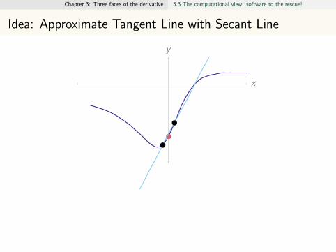
Idea: Approximate Tangent Line with Secant Line
x
y
secant
secant
secantsecantsecantsecantsecantsecantsecantsecantsecant
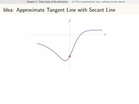
Derivative (slope of tangent line) limh→0
f (x + h)− f (x)
h
Approximate derivative Slope of secant linef (x + h)− f (x)
h
Chapter 3: Three faces of the derivative 3.3 The computational view: software to the rescue!
Idea: Approximate Tangent Line with Secant Line
x
y
secant
secant
secantsecantsecantsecantsecantsecantsecantsecantsecant
Derivative (slope of tangent line) limh→0
f (x + h)− f (x)
h
Approximate derivative Slope of secant linef (x + h)− f (x)
h
Chapter 3: Three faces of the derivative 3.3 The computational view: software to the rescue!
Idea: Approximate Tangent Line with Secant Line
x
y
secant
secant
secant
secantsecantsecantsecantsecantsecantsecantsecant
Derivative (slope of tangent line) limh→0
f (x + h)− f (x)
h
Approximate derivative Slope of secant linef (x + h)− f (x)
h

Chapter 3: Three faces of the derivative 3.3 The computational view: software to the rescue!
Idea: Approximate Tangent Line with Secant Line
x
y
secant
secant
secant
secant
secantsecantsecantsecantsecantsecantsecant
Derivative (slope of tangent line) limh→0
f (x + h)− f (x)
h
Approximate derivative Slope of secant linef (x + h)− f (x)
h

Chapter 3: Three faces of the derivative 3.3 The computational view: software to the rescue!
Idea: Approximate Tangent Line with Secant Line
x
y
secant
secant
secantsecant
secant
secantsecantsecantsecantsecantsecant
Derivative (slope of tangent line) limh→0
f (x + h)− f (x)
h
Approximate derivative Slope of secant linef (x + h)− f (x)
h
Chapter 3: Three faces of the derivative 3.3 The computational view: software to the rescue!
Idea: Approximate Tangent Line with Secant Line
x
y
secant
secant
secantsecantsecant
secant
secantsecantsecantsecantsecant
Derivative (slope of tangent line) limh→0
f (x + h)− f (x)
h
Approximate derivative Slope of secant linef (x + h)− f (x)
h
Chapter 3: Three faces of the derivative 3.3 The computational view: software to the rescue!
Idea: Approximate Tangent Line with Secant Line
x
y
secant
secant
secantsecantsecantsecant
secant
secantsecantsecantsecant
Derivative (slope of tangent line) limh→0
f (x + h)− f (x)
h
Approximate derivative Slope of secant linef (x + h)− f (x)
h
Chapter 3: Three faces of the derivative 3.3 The computational view: software to the rescue!
Idea: Approximate Tangent Line with Secant Line
x
y
secant
secant
secantsecantsecantsecantsecant
secant
secantsecantsecant
Derivative (slope of tangent line) limh→0
f (x + h)− f (x)
h
Approximate derivative Slope of secant linef (x + h)− f (x)
h
Chapter 3: Three faces of the derivative 3.3 The computational view: software to the rescue!
Idea: Approximate Tangent Line with Secant Line
x
y
secant
secant
secantsecantsecantsecantsecantsecant
secant
secantsecant
Derivative (slope of tangent line) limh→0
f (x + h)− f (x)
h
Approximate derivative Slope of secant linef (x + h)− f (x)
h

Chapter 3: Three faces of the derivative 3.3 The computational view: software to the rescue!
Idea: Approximate Tangent Line with Secant Line
x
y
secant
secant
secantsecantsecantsecantsecantsecantsecant
secant
secant
Derivative (slope of tangent line) limh→0
f (x + h)− f (x)
h
Approximate derivative Slope of secant linef (x + h)− f (x)
h

Chapter 3: Three faces of the derivative 3.3 The computational view: software to the rescue!
Idea: Approximate Tangent Line with Secant Line
x
y
secant
secant
secantsecantsecantsecantsecantsecantsecantsecant
secant
Derivative (slope of tangent line) limh→0
f (x + h)− f (x)
h
Approximate derivative Slope of secant linef (x + h)− f (x)
h
Chapter 3: Three faces of the derivative 3.3 The computational view: software to the rescue!
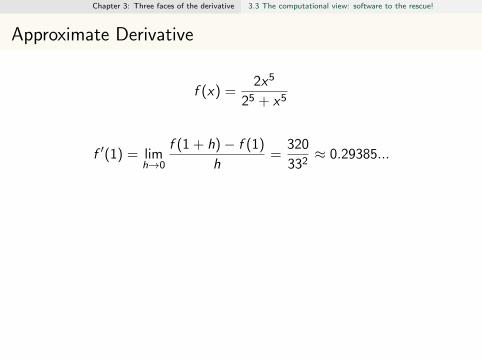
Approximate Derivative
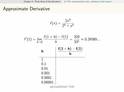
f (x) =2x5
25 + x5
f ′(1) = limh→0
f (1 + h)− f (1)
h=
320
332≈ 0.29385...
hf(1 + h)− f(1)
h
10.10.010.0010.00010.00001
spreadsheet link
Chapter 3: Three faces of the derivative 3.3 The computational view: software to the rescue!
Approximate Derivative
f (x) =2x5
25 + x5
f ′(1) = limh→0
f (1 + h)− f (1)
h=
320
332≈ 0.29385...
hf(1 + h)− f(1)
h
10.10.010.0010.00010.00001
spreadsheet link
Chapter 3: Three faces of the derivative 3.3 The computational view: software to the rescue!
Approximate Derivative
f (x) =2x5
25 + x5
f ′(1) = limh→0
f (1 + h)− f (1)
h=
320
332≈ 0.29385...
hf(1 + h)− f(1)
h
10.10.010.0010.00010.00001
spreadsheet link

Chapter 3: Three faces of the derivative 3.3 The computational view: software to the rescue!
Approximate Derivative
f (x) =2x5
25 + x5
f ′(1) = limh→0
f (1 + h)− f (1)
h=
320
332≈ 0.29385...
hf(1 + h)− f(1)
h
1 0.93939...0.1 0.35228...0.01 0.29932...0.001 0.29439...0.0001 0.29390...0.00001 0.29385...
spreadsheet link
Chapter 3: Three faces of the derivative 3.3 The computational view: software to the rescue!
Approximate Derivative
f (x) =2x5
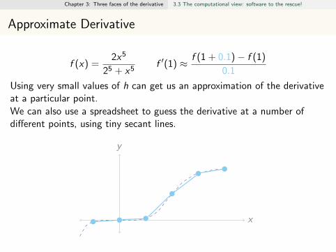
25 + x5f ′(1) ≈ f (1 + h)− f (1)
h
Using very small values of h can get us an approximation of the derivativeat a particular point.
We can also use a spreadsheet to guess the derivative at a number ofdifferent points, using tiny secant lines.
x
y
0.1 0.1
1
1.25
Chapter 3: Three faces of the derivative 3.3 The computational view: software to the rescue!
Approximate Derivative
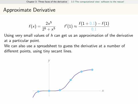
f (x) =2x5
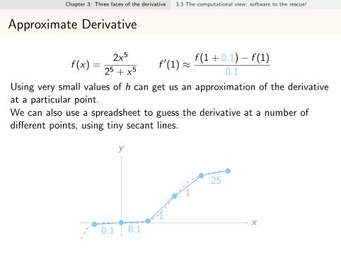
25 + x5f ′(1) ≈ f (1 + 0.1)− f (1)
0.1
Using very small values of h can get us an approximation of the derivativeat a particular point.
We can also use a spreadsheet to guess the derivative at a number ofdifferent points, using tiny secant lines.
x
y
0.1 0.1
1
1.25
Chapter 3: Three faces of the derivative 3.3 The computational view: software to the rescue!
Approximate Derivative
f (x) =2x5
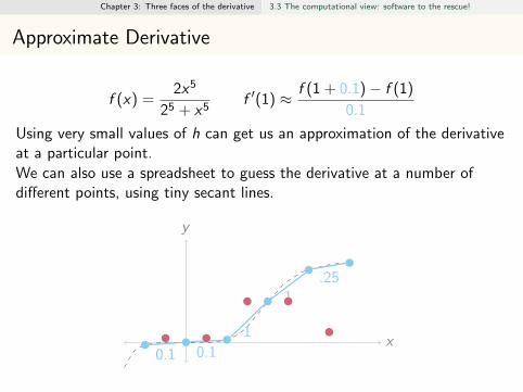
25 + x5f ′(1) ≈ f (1 + 0.1)− f (1)
0.1
Using very small values of h can get us an approximation of the derivativeat a particular point.
We can also use a spreadsheet to guess the derivative at a number ofdifferent points, using tiny secant lines.
x
y
0.1 0.1
1
1.25
Chapter 3: Three faces of the derivative 3.3 The computational view: software to the rescue!
Approximate Derivative
f (x) =2x5
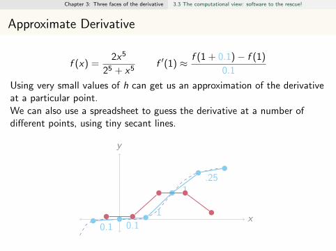
25 + x5f ′(1) ≈ f (1 + 0.1)− f (1)
0.1
Using very small values of h can get us an approximation of the derivativeat a particular point.
We can also use a spreadsheet to guess the derivative at a number ofdifferent points, using tiny secant lines.
x
y
0.1 0.1
1
1.25
Chapter 3: Three faces of the derivative 3.3 The computational view: software to the rescue!
Approximate Derivative
f (x) =2x5
25 + x5f ′(1) ≈ f (1 + 0.1)− f (1)
0.1
Using very small values of h can get us an approximation of the derivativeat a particular point.
We can also use a spreadsheet to guess the derivative at a number ofdifferent points, using tiny secant lines.
x
y
0.1 0.1
1
1.25

Chapter 3: Three faces of the derivative 3.3 The computational view: software to the rescue!
Approximate derivative at many points
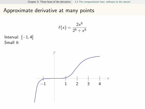
f (x) =2x5
25 + x5
Interval:
[−1, 4]
Small h:
say h = 0.1
x
y
−1 1 2 3 4
Chapter 3: Three faces of the derivative 3.3 The computational view: software to the rescue!
Approximate derivative at many points
f (x) =2x5
25 + x5
Interval: [−1, 4]Small h:
say h = 0.1
x
y
−1 1 2 3 4

Chapter 3: Three faces of the derivative 3.3 The computational view: software to the rescue!
Approximate derivative at many points
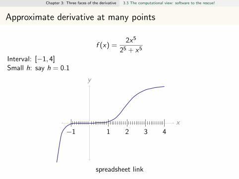
f (x) =2x5
25 + x5
Interval: [−1, 4]Small h: say h = 0.1
x
y
−1 1 2 3 4
Chapter 3: Three faces of the derivative 3.3 The computational view: software to the rescue!
Approximate derivative at many points
f (x) =2x5
25 + x5
Interval: [−1, 4]Small h: say h = 0.1
x
y
−1 1 2 3 4
spreadsheet link

Chapter 3: Three faces of the derivative 3.3 The computational view: software to the rescue!
Predator-Prey Interactions: Holling Predator Response
prey density
pred
atio
nra
te
P(x) =3x3
1 + x3
3
1
Type III: I can hardly find the prey when the prey density is low, but Ialso get satiated at high prey density.
(a) Label the asymptote on the y -axis.(b) Label the half-max activation level on the x-axis.
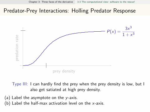
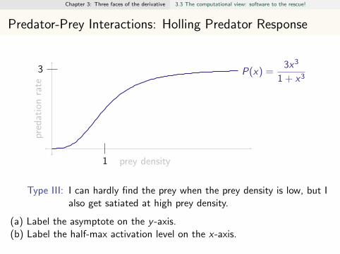
Chapter 3: Three faces of the derivative 3.3 The computational view: software to the rescue!
Predator-Prey Interactions: Holling Predator Response
prey density
pred
atio
nra
te
P(x) =3x3
1 + x33
1
Type III: I can hardly find the prey when the prey density is low, but Ialso get satiated at high prey density.
(a) Label the asymptote on the y -axis.(b) Label the half-max activation level on the x-axis.
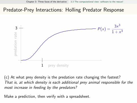
Chapter 3: Three faces of the derivative 3.3 The computational view: software to the rescue!
Predator-Prey Interactions: Holling Predator Response
prey density
pred
atio
nra
te
P(x) =3x3
1 + x33
1
(c) At what prey density is the predation rate changing the fastest?That is, at which density is each additional prey animal responsible for themost increase in feeding by the predators?
Make a prediction, then verify with a spreadsheet.
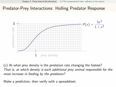