
Chapter 3: The Reinforcement Learning Problem (Markov...
46
R. S. Sutton and A. G. Barto: Reinforcement Learning: An Introduction Chapter 3: The Reinforcement Learning Problem (Markov Decision Processes, or MDPs) ❐ present Markov decision processes—an idealized form of the AI problem for which we have precise theoretical results ❐ introduce key components of the mathematics: value functions and Bellman equations Objectives of this chapter:
Transcript of Chapter 3: The Reinforcement Learning Problem (Markov...
R. S. Sutton and A. G. Barto: Reinforcement Learning: An Introduction
Chapter 3: The Reinforcement Learning Problem (Markov Decision Processes, or MDPs)
❐ present Markov decision processes—an idealized form of the AI problem for which we have precise theoretical results
❐ introduce key components of the mathematics: value functions and Bellman equations
Objectives of this chapter:
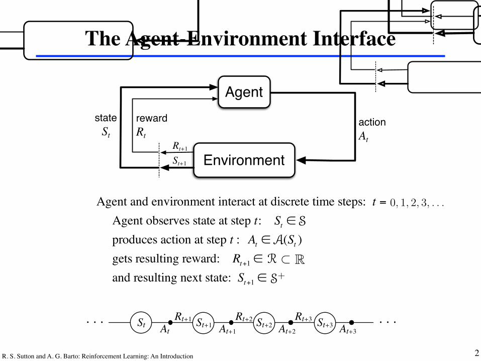
Agent and environment interact at discrete time steps: t = 0,1, 2,K Agent observes state at step t: St ∈ produces action at step t : At ∈ (St ) gets resulting reward: Rt+1 ∈
and resulting next state: St+1 ∈
Agent
Environment
actionAt
rewardRt
stateSt
Rt+1
St+1
AtRt+1St At+1
Rt+2St+1 At+2
Rt+3St+2 At+3St+3. . . . . .
R. S. Sutton and A. G. Barto: Reinforcement Learning: An Introduction 2
The Agent-Environment InterfaceSUMMARY OF NOTATION xiii
Summary of Notation
Capital letters are used for random variables and major algorithm variables.Lower case letters are used for the values of random variables and for scalarfunctions. Quantities that are required to be real-valued vectors are writtenin bold and in lower case (even if random variables).
s statea actionS set of all nonterminal statesS+ set of all states, including the terminal stateA(s) set of actions possible in state s
t discrete time stepT final time step of an episodeS
t
state at tA
t
action at tR
t
reward at t, dependent, like S
t
, on A
t�1
and S
t�1
G
t
return (cumulative discounted reward) following t
G
(n)
t
n-step return (Section 7.1)G
�
t
�-return (Section 7.2)
⇡ policy, decision-making rule⇡(s) action taken in state s under deterministic policy ⇡
⇡(a|s) probability of taking action a in state s under stochastic policy ⇡
p(s0|s, a) probability of transition from state s to state s
0 under action a
r(s, a, s0) expected immediate reward on transition from s to s
0 under action a
v
⇡
(s) value of state s under policy ⇡ (expected return)v⇤(s) value of state s under the optimal policyq
⇡
(s, a) value of taking action a in state s under policy ⇡
q⇤(s, a) value of taking action a in state s under the optimal policyV
t
estimate (a random variable) of v⇡
or v⇤Q
t
estimate (a random variable) of q⇡
or q⇤
v̂(s,w) approximate value of state s given a vector of weights wq̂(s, a,w) approximate value of state–action pair s, a given weights ww,w
t
vector of (possibly learned) weights underlying an approximate value functionx(s) vector of features visible when in state s
w>x inner product of vectors, w>x =P
i
w
i
x
i
; e.g., v̂(s,w) = w>x(s)
SUMMARY OF NOTATION xiii
Summary of Notation
Capital letters are used for random variables and major algorithm variables.Lower case letters are used for the values of random variables and for scalarfunctions. Quantities that are required to be real-valued vectors are writtenin bold and in lower case (even if random variables).
s statea actionS set of all nonterminal statesS+ set of all states, including the terminal stateA(s) set of actions possible in state s
t discrete time stepT final time step of an episodeS
t
state at tA
t
action at tR
t
reward at t, dependent, like S
t
, on A
t�1
and S
t�1
G
t
return (cumulative discounted reward) following t
G
(n)
t
n-step return (Section 7.1)G
�
t
�-return (Section 7.2)
⇡ policy, decision-making rule⇡(s) action taken in state s under deterministic policy ⇡
⇡(a|s) probability of taking action a in state s under stochastic policy ⇡
p(s0|s, a) probability of transition from state s to state s
0 under action a
r(s, a, s0) expected immediate reward on transition from s to s
0 under action a
v
⇡
(s) value of state s under policy ⇡ (expected return)v⇤(s) value of state s under the optimal policyq
⇡
(s, a) value of taking action a in state s under policy ⇡
q⇤(s, a) value of taking action a in state s under the optimal policyV
t
estimate (a random variable) of v⇡
or v⇤Q
t
estimate (a random variable) of q⇡
or q⇤
v̂(s,w) approximate value of state s given a vector of weights wq̂(s, a,w) approximate value of state–action pair s, a given weights ww,w
t
vector of (possibly learned) weights underlying an approximate value functionx(s) vector of features visible when in state s
w>x inner product of vectors, w>x =P
i
w
i
x
i
; e.g., v̂(s,w) = w>x(s)
R
! = s0
, a0
, s1
, a1
, . . .
The other random variables are a function of this sequence. The transitional
target rt+1
is a function of st, at, and st+1
. The termination condition �t,
terminal target zt, and prediction yt, are functions of st alone.
R(n)t = rt+1
+ �t+1
zt+1
+ (1� �t+1
)R(n�1)
t+1
R(0)
t = yt
R�t = (1� �)
1X
n=1
�n�1R(n)t
⇢t =⇡(st, at)
b(st, at)
�wo↵
(!) = �won
(!)1Y
i=1
⇢i
�wt = ↵t(CtR�t � yt)rwyt
�wt = ↵t(¯R�t � yt)rwyt
1
SUMMARY OF NOTATION xiii
Summary of Notation
Capital letters are used for random variables and major algorithm variables.Lower case letters are used for the values of random variables and for scalarfunctions. Quantities that are required to be real-valued vectors are writtenin bold and in lower case (even if random variables).
s statea actionS set of all nonterminal statesS+ set of all states, including the terminal stateA(s) set of actions possible in state s
t discrete time stepT final time step of an episodeS
t
state at tA
t
action at tR
t
reward at t, dependent, like S
t
, on A
t�1
and S
t�1
G
t
return (cumulative discounted reward) following t
G
(n)
t
n-step return (Section 7.1)G
�
t
�-return (Section 7.2)
⇡ policy, decision-making rule⇡(s) action taken in state s under deterministic policy ⇡
⇡(a|s) probability of taking action a in state s under stochastic policy ⇡
p(s0|s, a) probability of transition from state s to state s
0 under action a
r(s, a, s0) expected immediate reward on transition from s to s
0 under action a
v
⇡
(s) value of state s under policy ⇡ (expected return)v⇤(s) value of state s under the optimal policyq
⇡
(s, a) value of taking action a in state s under policy ⇡
q⇤(s, a) value of taking action a in state s under the optimal policyV
t
estimate (a random variable) of v⇡
or v⇤Q
t
estimate (a random variable) of q⇡
or q⇤
v̂(s,w) approximate value of state s given a vector of weights wq̂(s, a,w) approximate value of state–action pair s, a given weights ww,w
t
vector of (possibly learned) weights underlying an approximate value functionx(s) vector of features visible when in state s
w>x inner product of vectors, w>x =P
i
w
i
x
i
; e.g., v̂(s,w) = w>x(s)
44 CHAPTER 3. THE REINFORCEMENT LEARNING PROBLEM
Agent
Environment
actionAt
rewardRt
stateSt
Rt+1
St+1
Figure 3.1: The agent–environment interaction in reinforcement learning.
gives rise to rewards, special numerical values that the agent tries to maximizeover time. A complete specification of an environment defines a task , oneinstance of the reinforcement learning problem.
More specifically, the agent and environment interact at each of a sequenceof discrete time steps, t = 0, 1, 2, 3, . . ..2 At each time step t, the agent receivessome representation of the environment’s state, St 2 S, where S is the set ofpossible states, and on that basis selects an action, At 2 A(St), where A(St)is the set of actions available in state St. One time step later, in part as aconsequence of its action, the agent receives a numerical reward , Rt+1 2 R, andfinds itself in a new state, St+1.3 Figure 3.1 diagrams the agent–environmentinteraction.
At each time step, the agent implements a mapping from states to prob-abilities of selecting each possible action. This mapping is called the agent’spolicy and is denoted ⇡t, where ⇡t(a|s) is the probability that At = a if St = s.Reinforcement learning methods specify how the agent changes its policy asa result of its experience. The agent’s goal, roughly speaking, is to maximizethe total amount of reward it receives over the long run.
This framework is abstract and flexible and can be applied to many di↵erentproblems in many di↵erent ways. For example, the time steps need not referto fixed intervals of real time; they can refer to arbitrary successive stages ofdecision-making and acting. The actions can be low-level controls, such as thevoltages applied to the motors of a robot arm, or high-level decisions, suchas whether or not to have lunch or to go to graduate school. Similarly, thestates can take a wide variety of forms. They can be completely determined by
wider audience.2We restrict attention to discrete time to keep things as simple as possible, even though
many of the ideas can be extended to the continuous-time case (e.g., see Bertsekas andTsitsiklis, 1996; Werbos, 1992; Doya, 1996).
3We use Rt+1 instead of Rt to denote the immediate reward due to the action takenat time t because it emphasizes that the next reward and the next state, St+1, are jointlydetermined.
44 CHAPTER 3. THE REINFORCEMENT LEARNING PROBLEM
Agent
Environment
actionAt
rewardRt
stateSt
Rt+1
St+1
Figure 3.1: The agent–environment interaction in reinforcement learning.
gives rise to rewards, special numerical values that the agent tries to maximizeover time. A complete specification of an environment defines a task , oneinstance of the reinforcement learning problem.
More specifically, the agent and environment interact at each of a sequenceof discrete time steps, t = 0, 1, 2, 3, . . ..2 At each time step t, the agent receivessome representation of the environment’s state, St 2 S, where S is the set ofpossible states, and on that basis selects an action, At 2 A(St), where A(St)is the set of actions available in state St. One time step later, in part as aconsequence of its action, the agent receives a numerical reward , Rt+1 2 R ⇢R, where R is the set of possible rewards, and finds itself in a new state, St+1.3
Figure 3.1 diagrams the agent–environment interaction.
At each time step, the agent implements a mapping from states to prob-abilities of selecting each possible action. This mapping is called the agent’spolicy and is denoted ⇡t, where ⇡t(a|s) is the probability that At = a if St = s.Reinforcement learning methods specify how the agent changes its policy asa result of its experience. The agent’s goal, roughly speaking, is to maximizethe total amount of reward it receives over the long run.
This framework is abstract and flexible and can be applied to many di↵erentproblems in many di↵erent ways. For example, the time steps need not referto fixed intervals of real time; they can refer to arbitrary successive stages ofdecision-making and acting. The actions can be low-level controls, such as thevoltages applied to the motors of a robot arm, or high-level decisions, suchas whether or not to have lunch or to go to graduate school. Similarly, thestates can take a wide variety of forms. They can be completely determined by
wider audience.2We restrict attention to discrete time to keep things as simple as possible, even though
many of the ideas can be extended to the continuous-time case (e.g., see Bertsekas andTsitsiklis, 1996; Werbos, 1992; Doya, 1996).
3We use Rt+1 instead of Rt to denote the immediate reward due to the action takenat time t because it emphasizes that the next reward and the next state, St+1, are jointlydetermined.
R. S. Sutton and A. G. Barto: Reinforcement Learning: An Introduction 3
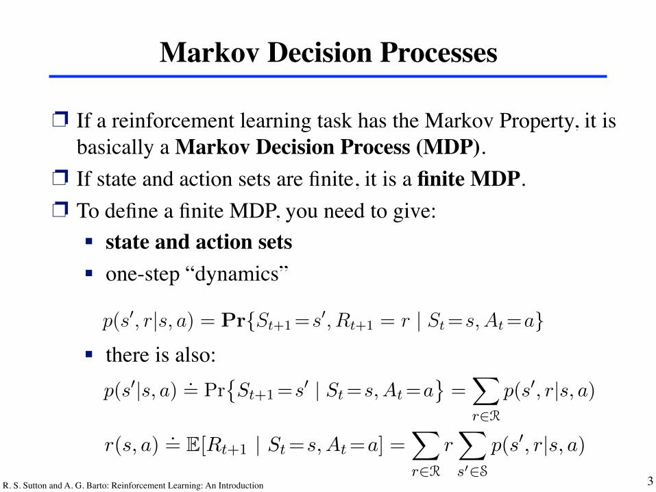
Markov Decision Processes
❐ If a reinforcement learning task has the Markov Property, it is basically a Markov Decision Process (MDP).
❐ If state and action sets are finite, it is a finite MDP. ❐ To define a finite MDP, you need to give:
! state and action sets! one-step “dynamics”
! there is also:
58 CHAPTER 3. THE REINFORCEMENT LEARNING PROBLEM
A particular finite MDP is defined by its state and action sets and by the
one-step dynamics of the environment. Given any state and action s and a,
the probability of each possible pair of next state and reward, s0, r, is denoted
p(s0, r|s, a) = Pr{St+1 =s0, Rt+1 = r | St =s, At =a}. (3.6)
These quantities completely specify the dynamics of a finite MDP. Most of the
theory we present in the rest of this book implicitly assumes the environment
is a finite MDP.
Given the dynamics as specified by (3.6), one can compute anything else
one might want to know about the environment, such as the expected rewards
for state–action pairs,
r(s, a) = E[Rt+1 | St =s, At =a] =
X
r2R
rX
s02S
p(s0, r|s, a), (3.7)
the state-transition probabilities,
p(s0|s, a) = Pr{St+1 =s0 | St =s, At =a} =
X
r2R
p(s0, r|s, a), (3.8)
and the expected rewards for state–action–next-state triples,
r(s, a, s0) = E[Rt+1 | St =s, At =a, St+1 = s0
] =
Pr2R rp(s0, r|s, a)
p(s0|s, a)
. (3.9)
In the first edition of this book, the dynamics were expressed exclusively in
terms of the latter two quantities, which were denote Pass0 and Ra
ss0 respectively.
One weakness of that notation is that it still did not fully characterize the
dynamics of the rewards, giving only their expectations. Another weakness is
the excess of subscripts and superscripts. In this edition we will predominantly
use the explicit notation of (3.6), while sometimes referring directly to the
transition probabilities (3.8).
Example 3.7: Recycling Robot MDP The recycling robot (Example
3.3) can be turned into a simple example of an MDP by simplifying it and
providing some more details. (Our aim is to produce a simple example, not
a particularly realistic one.) Recall that the agent makes a decision at times
determined by external events (or by other parts of the robot’s control system).
At each such time the robot decides whether it should (1) actively search for
a can, (2) remain stationary and wait for someone to bring it a can, or (3) go
back to home base to recharge its battery. Suppose the environment works
as follows. The best way to find cans is to actively search for them, but this
runs down the robot’s battery, whereas waiting does not. Whenever the robot
is searching, the possibility exists that its battery will become depleted. In
58 CHAPTER 3. FINITE MARKOV DECISION PROCESSES
3.6 Markov Decision Processes
A reinforcement learning task that satisfies the Markov property is called a Markovdecision process, or MDP. If the state and action spaces are finite, then it is called afinite Markov decision process (finite MDP). Finite MDPs are particularly importantto the theory of reinforcement learning. We treat them extensively throughout thisbook; they are all you need to understand 90% of modern reinforcement learning.
A particular finite MDP is defined by its state and action sets and by the one-stepdynamics of the environment. Given any state and action s and a, the probabilityof each possible pair of next state and reward, s0, r, is denoted
p(s0, r|s, a).= Pr
�St+1 =s0, Rt+1 = r | St =s, At =a
. (3.6)
These quantities completely specify the dynamics of a finite MDP. Most of the theorywe present in the rest of this book implicitly assumes the environment is a finite MDP.
Given the dynamics as specified by (3.6), one can compute anything else one mightwant to know about the environment, such as the expected rewards for state–actionpairs,
r(s, a).= E[Rt+1 | St =s, At =a] =
X
r2R
rX
s02S
p(s0, r|s, a), (3.7)
the state-transition probabilities,
p(s0|s, a).= Pr
�St+1 =s0 | St =s, At =a
=X
r2R
p(s0, r|s, a), (3.8)
and the expected rewards for state–action–next-state triples,
r(s, a, s0).= E
⇥Rt+1
�� St =s, At =a, St+1 = s0⇤ =
Pr2R rp(s0, r|s, a)
p(s0|s, a). (3.9)
In the first edition of this book, the dynamics were expressed exclusively in termsof the latter two quantities, which were denoted Pa
ss0 and Rass0 respectively. One
weakness of that notation is that it still did not fully characterize the dynamicsof the rewards, giving only their expectations. Another weakness is the excess ofsubscripts and superscripts. In this edition we will predominantly use the explicitnotation of (3.6), while sometimes referring directly to the transition probabilities(3.8).
Example 3.7: Recycling Robot MDP The recycling robot (Example 3.3) canbe turned into a simple example of an MDP by simplifying it and providing somemore details. (Our aim is to produce a simple example, not a particularly realisticone.) Recall that the agent makes a decision at times determined by external events(or by other parts of the robot’s control system). At each such time the robot decideswhether it should (1) actively search for a can, (2) remain stationary and wait forsomeone to bring it a can, or (3) go back to home base to recharge its battery.Suppose the environment works as follows. The best way to find cans is to actively
R. S. Sutton and A. G. Barto: Reinforcement Learning: An Introduction 4
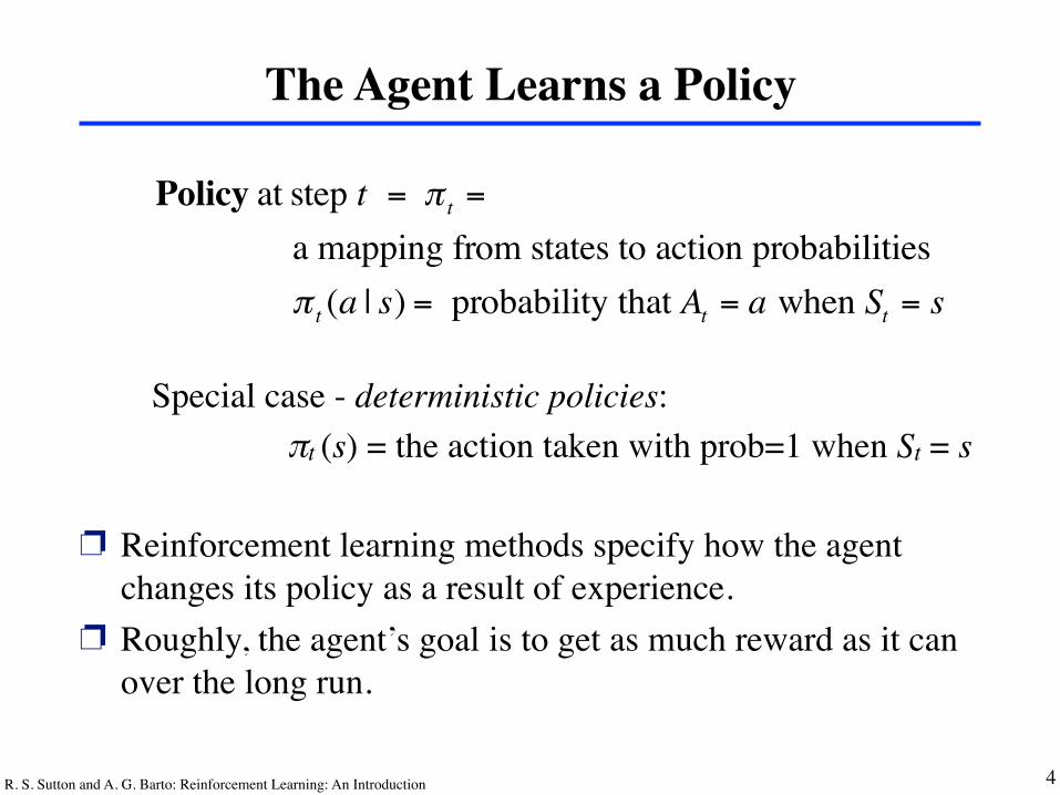
Policy at step t = π t =
a mapping from states to action probabilities π t (a | s) = probability that At = a when St = s
The Agent Learns a Policy
❐ Reinforcement learning methods specify how the agent changes its policy as a result of experience.
❐ Roughly, the agent’s goal is to get as much reward as it can over the long run.
Special case - deterministic policies: πt (s) = the action taken with prob=1 when St = s
R. S. Sutton and A. G. Barto: Reinforcement Learning: An Introduction 5
The Meaning of Life(goals, rewards, and returns)
R. S. Sutton and A. G. Barto: Reinforcement Learning: An Introduction 6
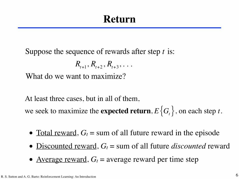
Return
Suppose the sequence of rewards after step t is: Rt+1, Rt+2 , Rt+3,KWhat do we want to maximize?
At least three cases, but in all of them, we seek to maximize the expected return, E Gt{ }, on each step t.
• Total reward, Gt = sum of all future reward in the episode
• Discounted reward, Gt = sum of all future discounted reward
• Average reward, Gt = average reward per time step
. . .
R. S. Sutton and A. G. Barto: Reinforcement Learning: An Introduction
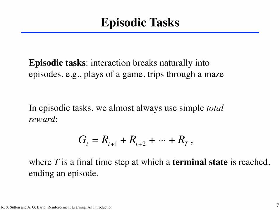
Episodic Tasks
7
Episodic tasks: interaction breaks naturally into episodes, e.g., plays of a game, trips through a maze
In episodic tasks, we almost always use simple total reward:
Gt = Rt+1 + Rt+2 +L + RT ,
where T is a final time step at which a terminal state is reached, ending an episode.
...
R. S. Sutton and A. G. Barto: Reinforcement Learning: An Introduction 8
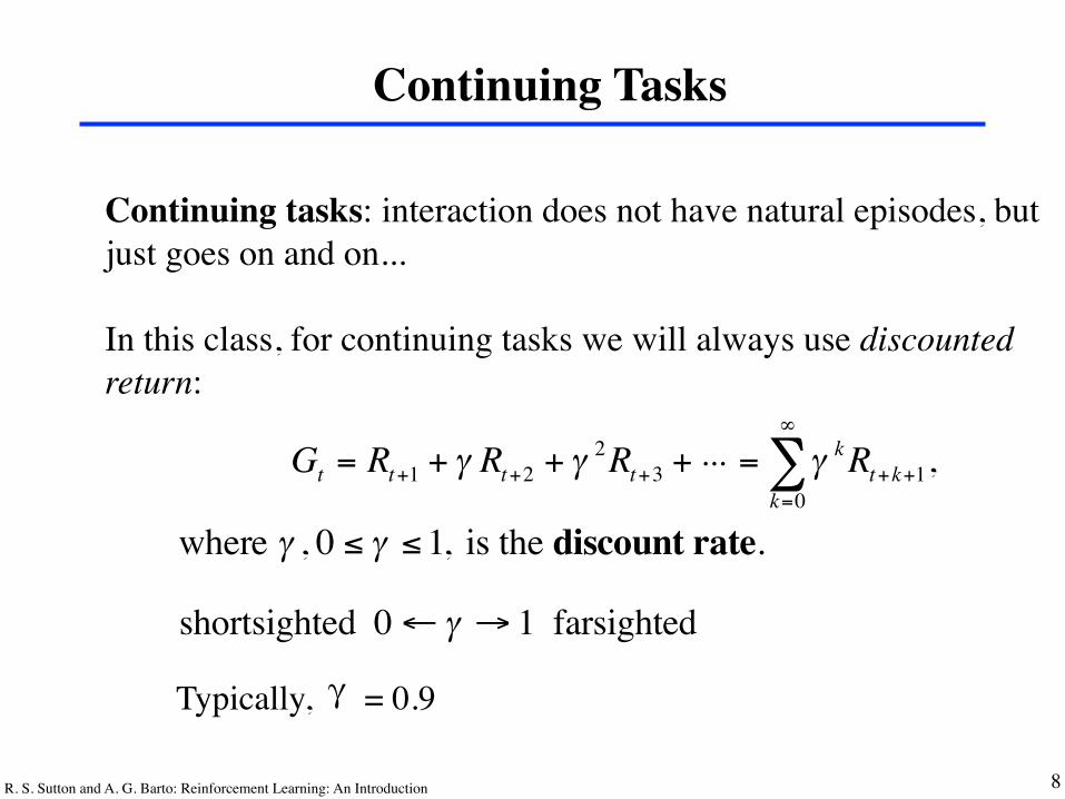
Continuing Tasks
Continuing tasks: interaction does not have natural episodes, but just goes on and on...
In this class, for continuing tasks we will always use discounted return:
Gt = Rt+1 + γ Rt+2 + γ2Rt+3 +L = γ kRt+k+1,
k=0
∞
∑where γ , 0 ≤ γ ≤1, is the discount rate.
shortsighted 0 ←γ → 1 farsighted
Typically, � = 0.9
...
R. S. Sutton and A. G. Barto: Reinforcement Learning: An Introduction 9
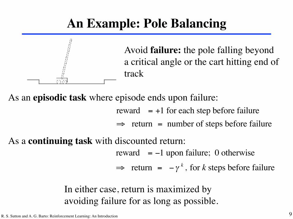
An Example: Pole Balancing
Avoid failure: the pole falling beyonda critical angle or the cart hitting end oftrack
reward = +1 for each step before failure⇒ return = number of steps before failure
As an episodic task where episode ends upon failure:
As a continuing task with discounted return:reward = −1 upon failure; 0 otherwise
⇒ return = −γ k , for k steps before failure
In either case, return is maximized by avoiding failure for as long as possible.
R. S. Sutton and A. G. Barto: Reinforcement Learning: An Introduction 10
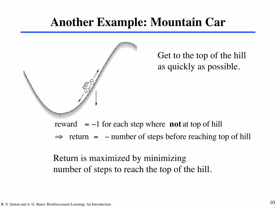
Another Example: Mountain Car
Get to the top of the hillas quickly as possible.
reward = −1 for each step where not at top of hill⇒ return = − number of steps before reaching top of hill
Return is maximized by minimizing number of steps to reach the top of the hill.
R1 = +1S0 S1R2 = +1 S2
R3 = +1 R4 = 0R5 = 0. . .
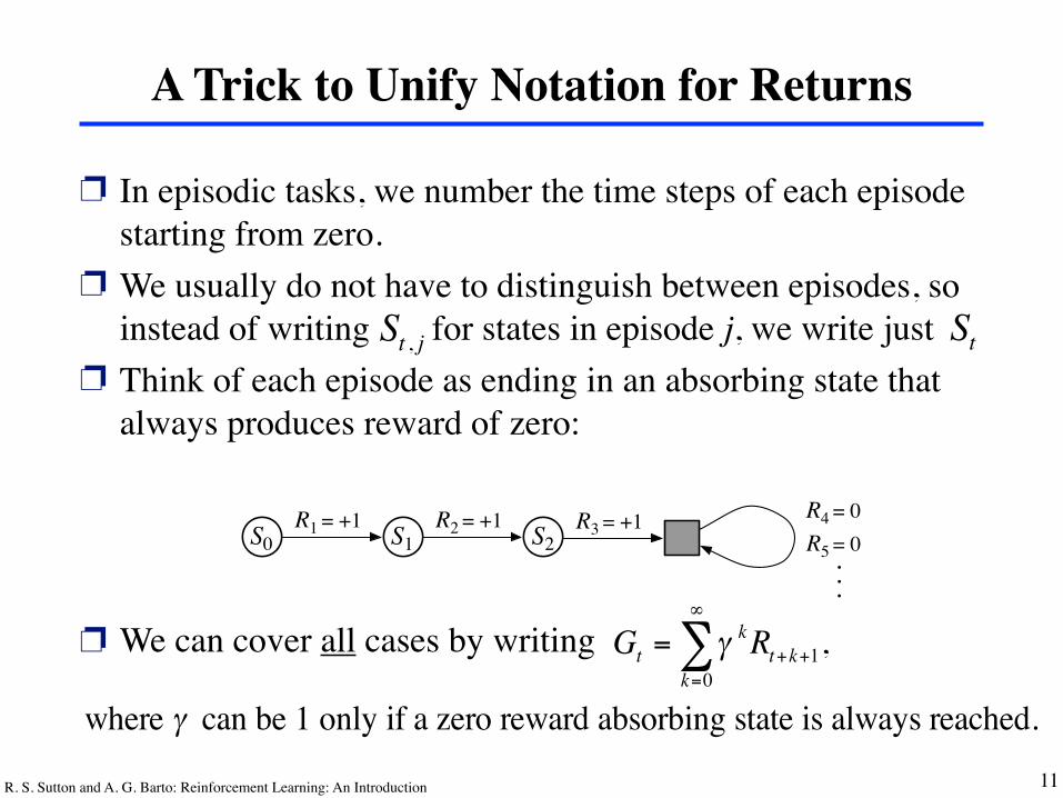
❐ In episodic tasks, we number the time steps of each episode starting from zero.
❐ We usually do not have to distinguish between episodes, so instead of writing for states in episode j, we write just
❐ Think of each episode as ending in an absorbing state that always produces reward of zero:
❐ We can cover all cases by writing
R. S. Sutton and A. G. Barto: Reinforcement Learning: An Introduction 11
A Trick to Unify Notation for Returns
StSt , j
Gt = γ kRt+k+1,k=0
∞
∑where γ can be 1 only if a zero reward absorbing state is always reached.
Rewards and returns• The objective in RL is to maximize long-term future reward
• That is, to choose so as to maximize
• But what exactly should be maximized?
• The discounted return at time t:
At Rt+1, Rt+2, Rt+3, . . .
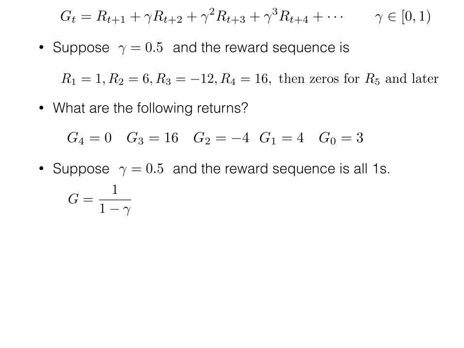
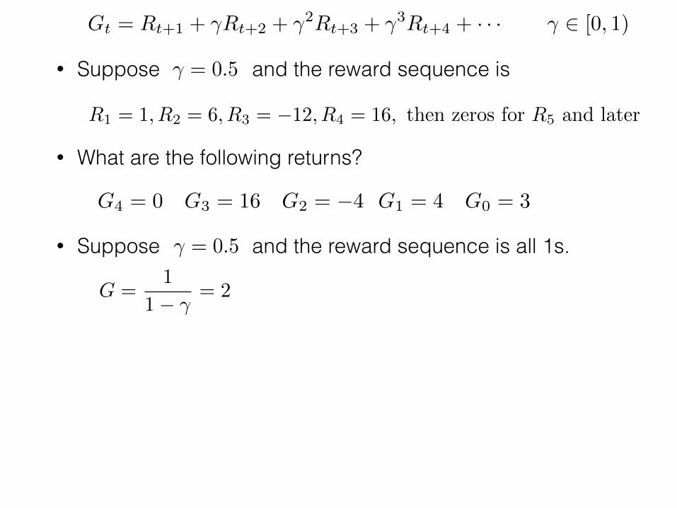
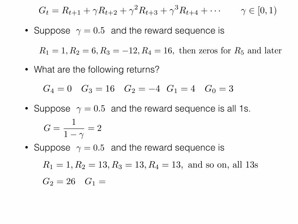
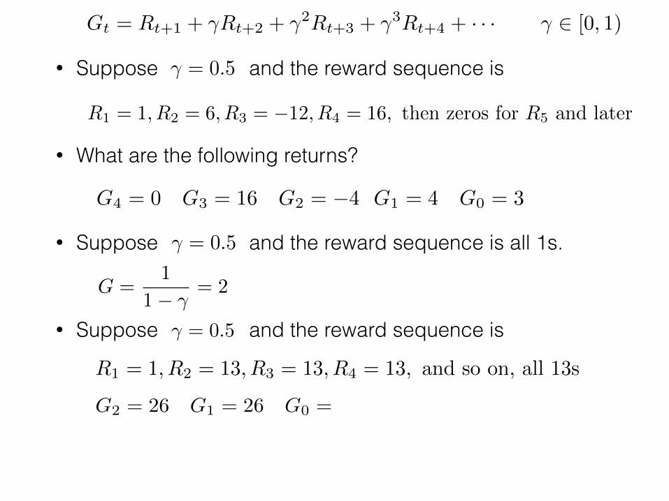
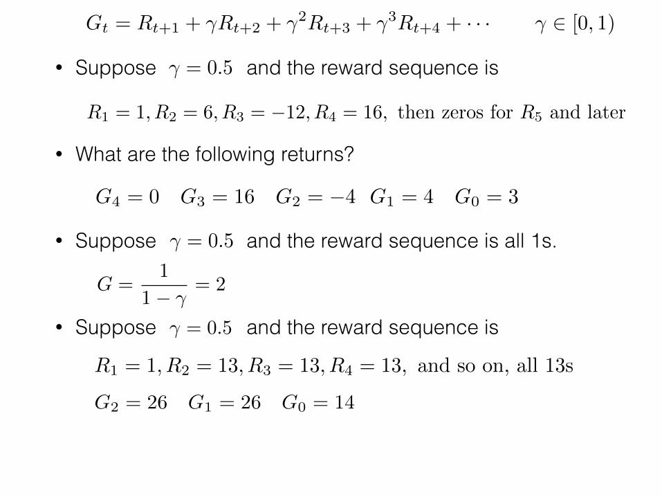
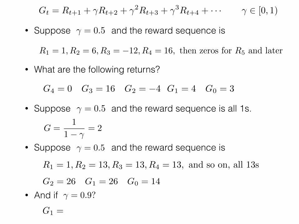
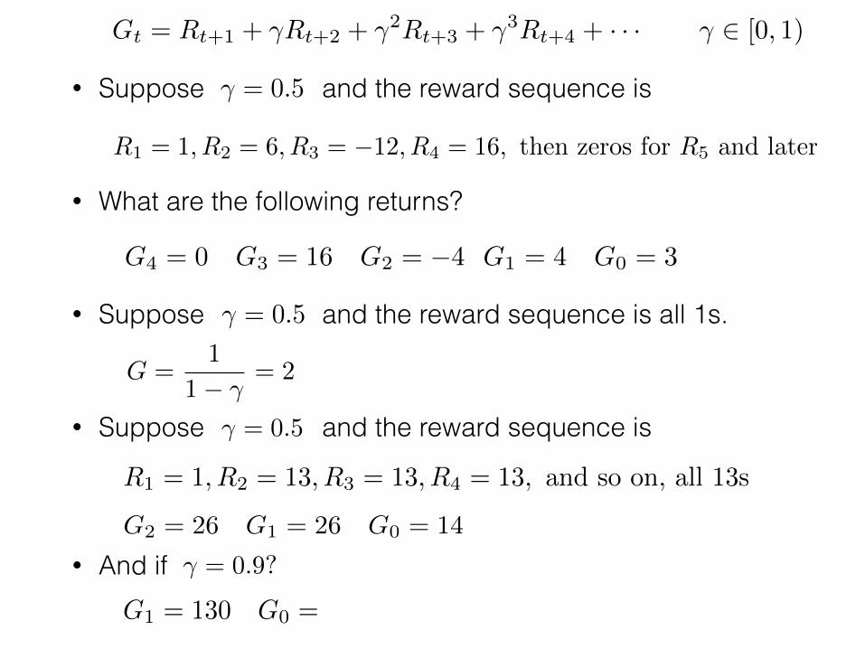
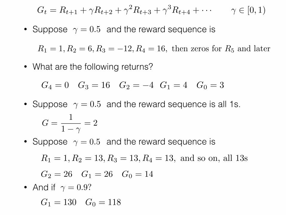
Gt = Rt+1 + �Rt+2 + �2Rt+3 + �3Rt+4 + · · · � 2 [0, 1)
Reward sequence1 0 0 0…
Return1
0 0 2 0 0 0…0.5(or any)
0.5 0.50.9 0 0 2 0 0 0… 1.620.5 -1 2 6 3 2 0 0 0… 2
�
the discount rate
• Suppose and the reward sequence is
• What are the following returns?
• Suppose and the reward sequence is all 1s.
• Suppose and the reward sequence is
• And if
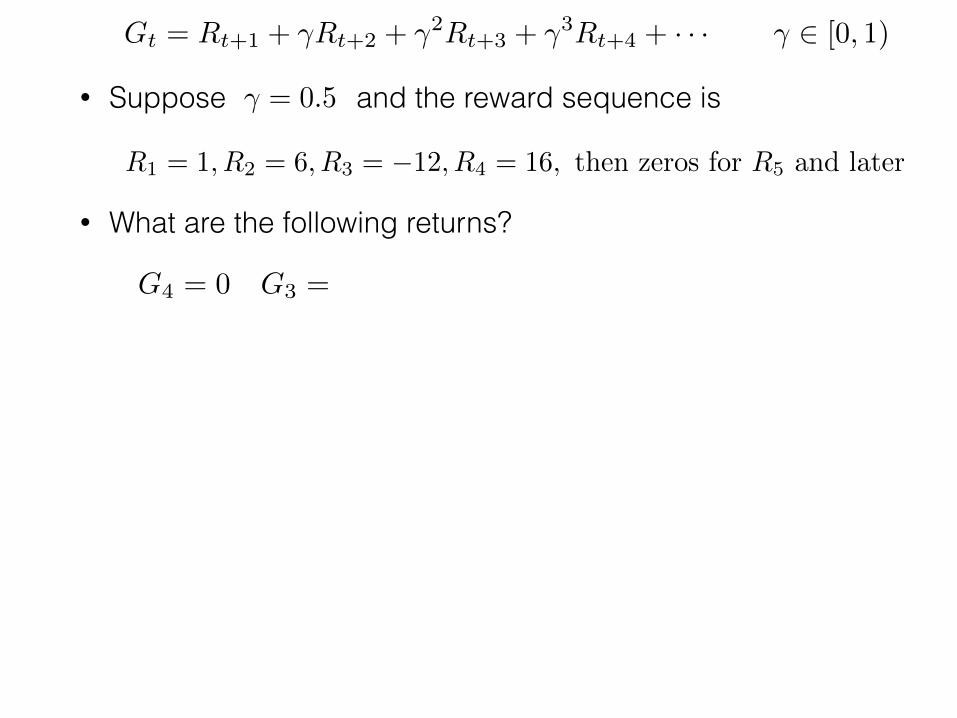
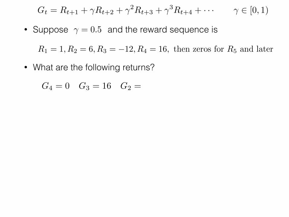
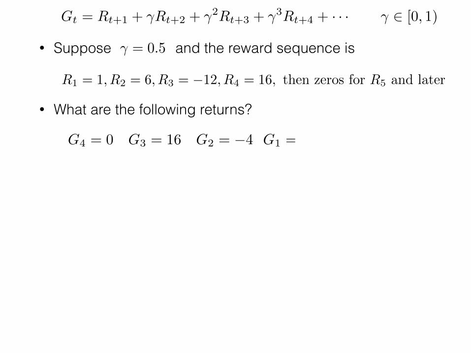
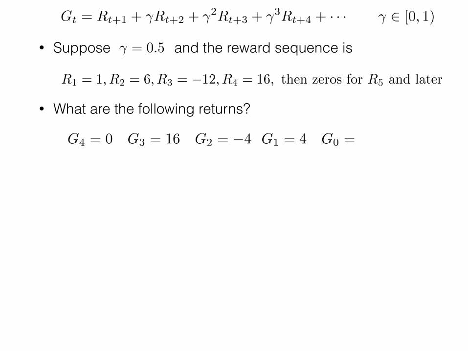
Gt = Rt+1 + �Rt+2 + �2Rt+3 + �3Rt+4 + · · · � 2 [0, 1)
R1 = 1, R2 = 6, R3 = �12, R4 = 16, then zeros for R5 and later
� = 0.5
G4 = 0 G3 = 16 G2 = �4 G1 = 4 G0 = 3
� = 0.5
R1 = 1, R2 = 13, R3 = 13, R4 = 13, and so on, all 13s
G =1
1� �= 2
� = 0.5
G2 = 26 G1 = 26 G0 = 14
� = 0.9?
G1 = 130 G0 = 118
• Suppose and the reward sequence is
• What are the following returns?
• Suppose and the reward sequence is all 1s.
• Suppose and the reward sequence is
• And if
Gt = Rt+1 + �Rt+2 + �2Rt+3 + �3Rt+4 + · · · � 2 [0, 1)
R1 = 1, R2 = 6, R3 = �12, R4 = 16, then zeros for R5 and later
� = 0.5
G4 = 0 G3 = 16 G2 = �4 G1 = 4 G0 = 3
� = 0.5
R1 = 1, R2 = 13, R3 = 13, R4 = 13, and so on, all 13s
G =1
1� �= 2
� = 0.5
G2 = 26 G1 = 26 G0 = 14
� = 0.9?
G1 = 130 G0 = 118

• Suppose and the reward sequence is
• What are the following returns?
• Suppose and the reward sequence is all 1s.
• Suppose and the reward sequence is
• And if
Gt = Rt+1 + �Rt+2 + �2Rt+3 + �3Rt+4 + · · · � 2 [0, 1)
R1 = 1, R2 = 6, R3 = �12, R4 = 16, then zeros for R5 and later
� = 0.5
G4 = 0 G3 = 16 G2 = �4 G1 = 4 G0 = 3
� = 0.5
R1 = 1, R2 = 13, R3 = 13, R4 = 13, and so on, all 13s
G =1
1� �= 2
� = 0.5
G2 = 26 G1 = 26 G0 = 14
� = 0.9?
G1 = 130 G0 = 118
• Suppose and the reward sequence is
• What are the following returns?
• Suppose and the reward sequence is all 1s.
• Suppose and the reward sequence is
• And if
Gt = Rt+1 + �Rt+2 + �2Rt+3 + �3Rt+4 + · · · � 2 [0, 1)
R1 = 1, R2 = 6, R3 = �12, R4 = 16, then zeros for R5 and later
� = 0.5
G4 = 0 G3 = 16 G2 = �4 G1 = 4 G0 = 3
� = 0.5
R1 = 1, R2 = 13, R3 = 13, R4 = 13, and so on, all 13s
G =1
1� �= 2
� = 0.5
G2 = 26 G1 = 26 G0 = 14
� = 0.9?
G1 = 130 G0 = 118

• Suppose and the reward sequence is
• What are the following returns?
• Suppose and the reward sequence is all 1s.
• Suppose and the reward sequence is
• And if
Gt = Rt+1 + �Rt+2 + �2Rt+3 + �3Rt+4 + · · · � 2 [0, 1)
R1 = 1, R2 = 6, R3 = �12, R4 = 16, then zeros for R5 and later
� = 0.5
G4 = 0 G3 = 16 G2 = �4 G1 = 4 G0 = 3
� = 0.5
R1 = 1, R2 = 13, R3 = 13, R4 = 13, and so on, all 13s
G =1
1� �= 2
� = 0.5
G2 = 26 G1 = 26 G0 = 14
� = 0.9?
G1 = 130 G0 = 118
• Suppose and the reward sequence is
• What are the following returns?
• Suppose and the reward sequence is all 1s.
• Suppose and the reward sequence is
• And if
Gt = Rt+1 + �Rt+2 + �2Rt+3 + �3Rt+4 + · · · � 2 [0, 1)
R1 = 1, R2 = 6, R3 = �12, R4 = 16, then zeros for R5 and later
� = 0.5
G4 = 0 G3 = 16 G2 = �4 G1 = 4 G0 = 3
� = 0.5
R1 = 1, R2 = 13, R3 = 13, R4 = 13, and so on, all 13s
G =1
1� �= 2
� = 0.5
G2 = 26 G1 = 26 G0 = 14
� = 0.9?
G1 = 130 G0 = 118
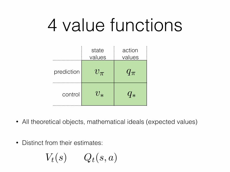
4 value functions
• All theoretical objects, mathematical ideals (expected values)
• Distinct from their estimates:
state values
action values
prediction
control q⇤v⇤
v⇡ q⇡
Vt(s) Qt(s, a)
Values are expected returns• The value of a state, given a policy:
• The value of a state-action pair, given a policy:
• The optimal value of a state:
• The optimal value of a state-action pair:
• Optimal policy: is an optimal policy if and only if
• in other words, is optimal iff it is greedy wrt
v⇡(s) = E{Gt | St = s,At:1⇠⇡} v⇡ : S ! <
q⇡(s, a) = E{Gt | St = s,At = a,At+1:1⇠⇡} q⇡ : S⇥A ! <
v⇤(s) = max
⇡v⇡(s) v⇤ : S ! <
⇡⇤(a|s) > 0 only where q⇤(s, a) = max
bq⇤(s, b)
⇡⇤
⇡⇤ q⇤
8s 2 S
q⇤(s, a) = max
⇡q⇡(s, a) q⇤ : S⇥A ! <

4 value functions
• All theoretical objects, mathematical ideals (expected values)
• Distinct from their estimates:
state values
action values
prediction
control q⇤v⇤
v⇡ q⇡
Vt(s) Qt(s, a)
R. S. Sutton and A. G. Barto: Reinforcement Learning: An Introduction
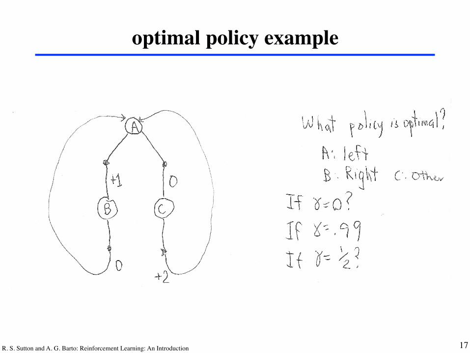
optimal policy example
17

R. S. Sutton and A. G. Barto: Reinforcement Learning: An Introduction 18
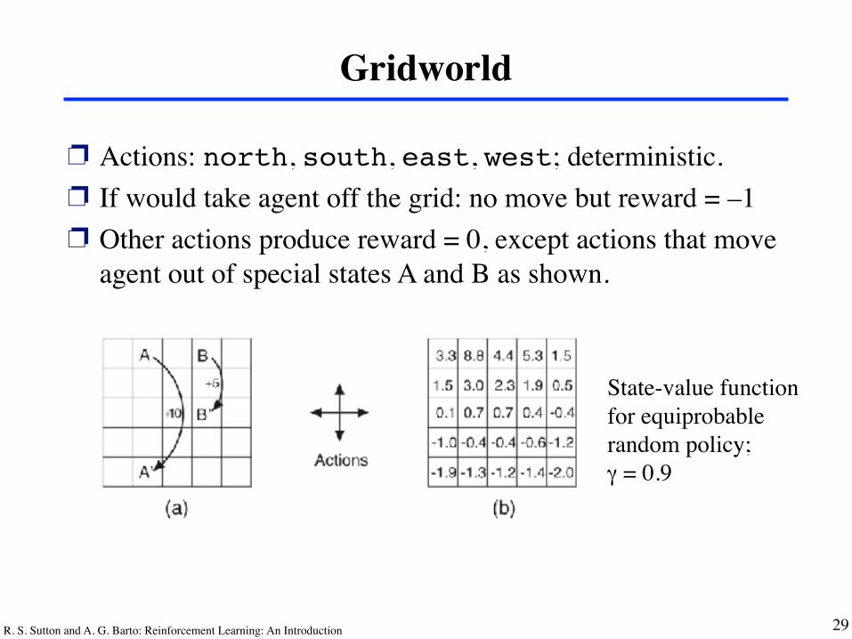
Gridworld
❐ Actions: north, south, east, west; deterministic.❐ If would take agent off the grid: no move but reward = –1❐ Other actions produce reward = 0, except actions that move
agent out of special states A and B as shown.
State-value function for equiprobable random policy;γ = 0.9
R. S. Sutton and A. G. Barto: Reinforcement Learning: An Introduction 19
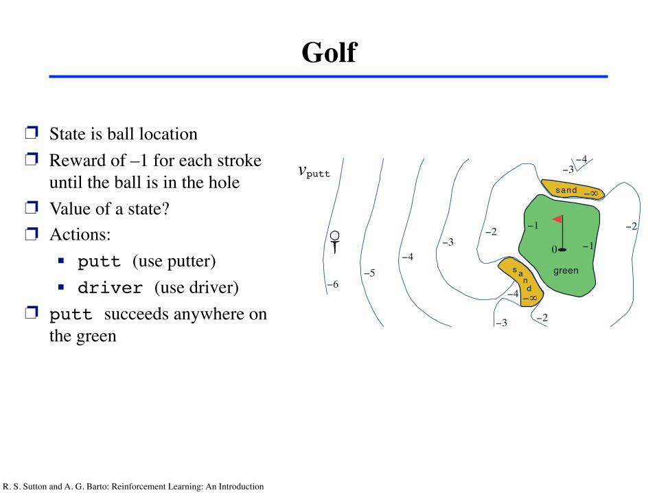
Golf
❐ State is ball location❐ Reward of –1 for each stroke
until the ball is in the hole❐ Value of a state?❐ Actions:
! putt (use putter)! driver (use driver)
❐ putt succeeds anywhere on the green
Q*(s,driver)
Vputt
sand
green
!1
sand
!2!2
!3
!4
!1
!5!6
!4
!3
!3!2
!4
sand
green
!1
sand
!2
!3
!2
0
0
!"
!"
vputt
q*(s,driver)
R. S. Sutton and A. G. Barto: Reinforcement Learning: An Introduction
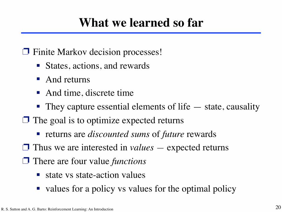
What we learned so far
❐ Finite Markov decision processes!! States, actions, and rewards! And returns! And time, discrete time! They capture essential elements of life — state, causality
❐ The goal is to optimize expected returns! returns are discounted sums of future rewards
❐ Thus we are interested in values — expected returns❐ There are four value functions
! state vs state-action values! values for a policy vs values for the optimal policy
20
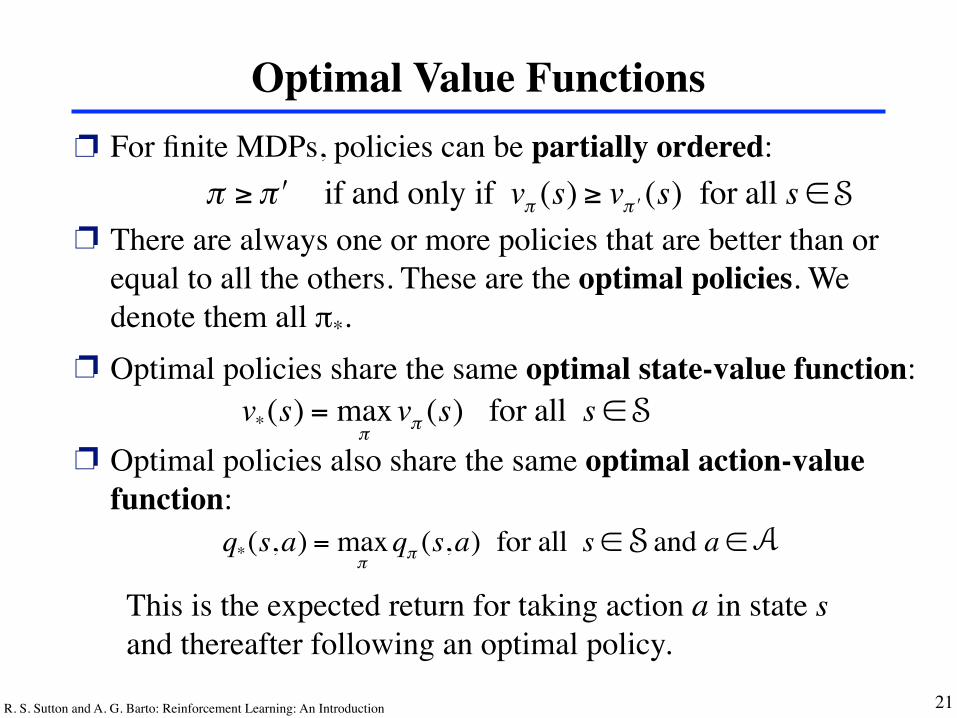
R. S. Sutton and A. G. Barto: Reinforcement Learning: An Introduction 21
π ≥ #π if and only if vπ (s) ≥ vπ # (s) for all s ∈
Optimal Value Functions
v*(s) = maxπvπ (s) for all s ∈
q*(s,a) = maxπqπ (s,a) for all s ∈ and a∈ (s)
This is the expected return for taking action a in state s and thereafter following an optimal policy.
❐ For finite MDPs, policies can be partially ordered:
❐ There are always one or more policies that are better than or equal to all the others. These are the optimal policies. We denote them all π*.
❐ Optimal policies share the same optimal state-value function:
❐ Optimal policies also share the same optimal action-value function:
SUMMARY OF NOTATION xiii
Summary of Notation
Capital letters are used for random variables and major algorithm variables.Lower case letters are used for the values of random variables and for scalarfunctions. Quantities that are required to be real-valued vectors are writtenin bold and in lower case (even if random variables).
s statea actionS set of all nonterminal statesS+ set of all states, including the terminal stateA(s) set of actions possible in state s
t discrete time stepT final time step of an episodeS
t
state at tA
t
action at tR
t
reward at t, dependent, like S
t
, on A
t�1
and S
t�1
G
t
return (cumulative discounted reward) following t
G
(n)
t
n-step return (Section 7.1)G
�
t
�-return (Section 7.2)
⇡ policy, decision-making rule⇡(s) action taken in state s under deterministic policy ⇡
⇡(a|s) probability of taking action a in state s under stochastic policy ⇡
p(s0|s, a) probability of transition from state s to state s
0 under action a
r(s, a, s0) expected immediate reward on transition from s to s
0 under action a
v
⇡
(s) value of state s under policy ⇡ (expected return)v⇤(s) value of state s under the optimal policyq
⇡
(s, a) value of taking action a in state s under policy ⇡
q⇤(s, a) value of taking action a in state s under the optimal policyV
t
estimate (a random variable) of v⇡
or v⇤Q
t
estimate (a random variable) of q⇡
or q⇤
v̂(s,w) approximate value of state s given a vector of weights wq̂(s, a,w) approximate value of state–action pair s, a given weights ww,w
t
vector of (possibly learned) weights underlying an approximate value functionx(s) vector of features visible when in state s
w>x inner product of vectors, w>x =P
i
w
i
x
i
; e.g., v̂(s,w) = w>x(s)

R. S. Sutton and A. G. Barto: Reinforcement Learning: An Introduction 22
Why Optimal State-Value Functions are Useful
v*
v*
Any policy that is greedy with respect to is an optimal policy.
Therefore, given , one-step-ahead search produces the long-term optimal actions.
E.g., back to the gridworld:
a) gridworld b) V* c) !*
22.0 24.4 22.0 19.4 17.5
19.8 22.0 19.8 17.8 16.0
17.8 19.8 17.8 16.0 14.4
16.0 17.8 16.0 14.4 13.0
14.4 16.0 14.4 13.0 11.7
A B
A'
B'+10
+5
v* π*
R. S. Sutton and A. G. Barto: Reinforcement Learning: An Introduction 23
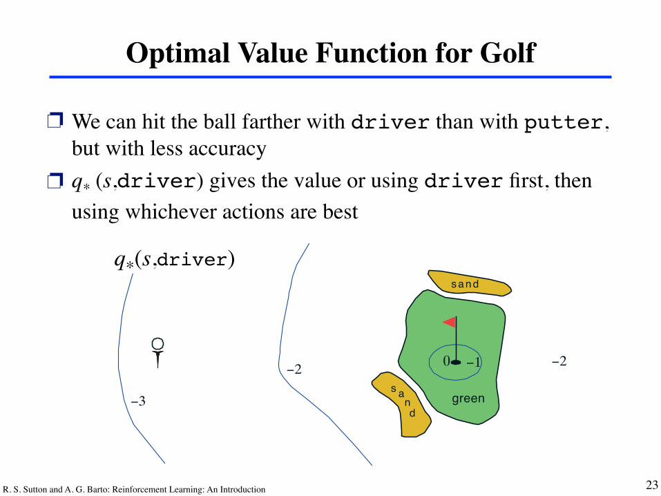
Optimal Value Function for Golf
❐ We can hit the ball farther with driver than with putter, but with less accuracy
❐ q* (s,driver) gives the value or using driver first, then using whichever actions are best
Q*(s,driver)
Vputt
sand
green
!1
sand
!2!2
!3
!4
!1
!5!6
!4
!3
!3!2
!4
sand
green
!1
sand
!2
!3
!2
0
0
!"
!"
vputt
q*(s,driver)
R. S. Sutton and A. G. Barto: Reinforcement Learning: An Introduction 24
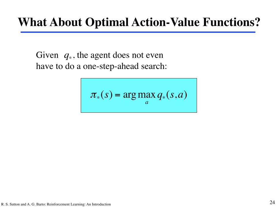
What About Optimal Action-Value Functions?
Given , the agent does not evenhave to do a one-step-ahead search:
q*
π*(s) = argmaxa q*(s,a)
R. S. Sutton and A. G. Barto: Reinforcement Learning: An Introduction 25
Value Functionsx 4
R. S. Sutton and A. G. Barto: Reinforcement Learning: An Introduction 26
Bellman Equationsx 4

R. S. Sutton and A. G. Barto: Reinforcement Learning: An Introduction 27
Bellman Equation for a Policy π
Gt = Rt+1 + γ Rt+2 + γ2Rt+3 + γ
3Rt+4L= Rt+1 + γ Rt+2 + γ Rt+3 + γ
2Rt+4L( )= Rt+1 + γGt+1
The basic idea:
So: vπ (s) = Eπ Gt St = s{ }= Eπ Rt+1 + γ vπ St+1( ) St = s{ }
Or, without the expectation operator:
...+
...+
v⇡(s) =X
a
⇡(a|s)X
s0,r
p(s0, r|s, a)hr + �v⇡(s
0)i
v⇡(s) = E⇡
⇥Rt+1 + �Rt+2 + �2Rt+3 + · · ·
�� St=s⇤
= E⇡[Rt+1 + �v⇡(St+1) | St=s] (1)
=X
a
⇡(a|s)X
s0,r
p(s0, r|s, a)hr + �v⇡(s
0)i, (2)
i
R. S. Sutton and A. G. Barto: Reinforcement Learning: An Introduction 28
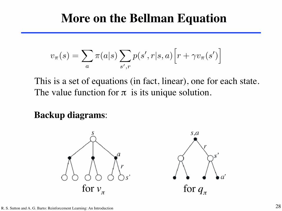
More on the Bellman Equation
This is a set of equations (in fact, linear), one for each state.The value function for π is its unique solution.
Backup diagrams:
for vπ for qπ
v⇡(s) =X
a
⇡(a|s)X
s0,r
p(s0, r|s, a)hr + �v⇡(s
0)i
v⇡(s) = E⇡
⇥Rt+1 + �Rt+2 + �2Rt+3 + · · ·
�� St=s⇤
= E⇡[Rt+1 + �v⇡(St+1) | St=s] (1)
=X
a
⇡(a|s)X
s0,r
p(s0, r|s, a)hr + �v⇡(s
0)i, (2)
i
R. S. Sutton and A. G. Barto: Reinforcement Learning: An Introduction 29
Gridworld
❐ Actions: north, south, east, west; deterministic.❐ If would take agent off the grid: no move but reward = –1❐ Other actions produce reward = 0, except actions that move
agent out of special states A and B as shown.
State-value function for equiprobable random policy;γ = 0.9
R. S. Sutton and A. G. Barto: Reinforcement Learning: An Introduction 30
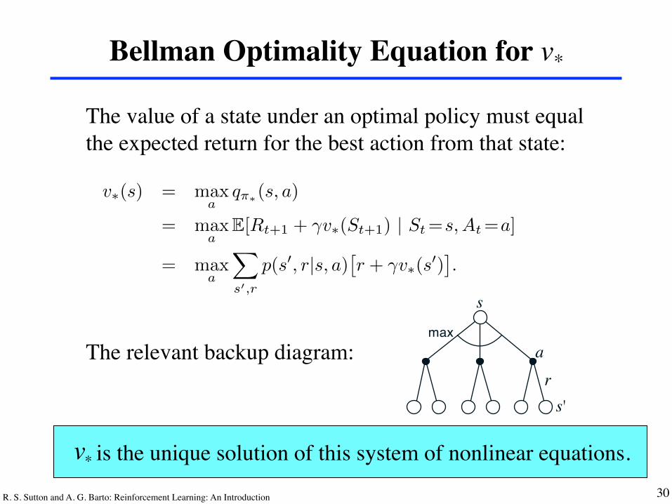
Bellman Optimality Equation for v*
The value of a state under an optimal policy must equalthe expected return for the best action from that state:
The relevant backup diagram:
is the unique solution of this system of nonlinear equations.v*
s,as
a
s'
r
a'
s'
r
(b)(a)
max
max
v⇡(s) =X
a
⇡(a|s)X
s0,r
p(s0, r|s, a)hr + �v⇡(s
0)
i
v⇡(s) = E⇡
⇥Rt+1 + �Rt+2 + �2Rt+3 + · · ·
�� St=s⇤
= E⇡[Rt+1 + �v⇡(St+1) | St=s] (1)
=
X
a
⇡(a|s)X
s0,r
p(s0, r|s, a)hr + �v⇡(s
0)
i, (2)
v⇤(s) = max
aq⇡⇤(s, a)
= max
aE[Rt+1 + �v⇤(St+1) | St=s,At=a] (3)
= max
a
X
s0,r
p(s0, r|s, a)⇥r + �v⇤(s
0)
⇤. (4)
i
R. S. Sutton and A. G. Barto: Reinforcement Learning: An Introduction 31
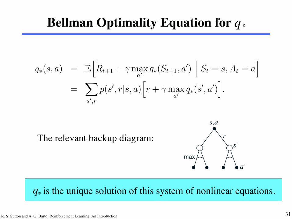
Bellman Optimality Equation for q*
The relevant backup diagram:
is the unique solution of this system of nonlinear equations.q*
s,as
a
s'
r
a'
s'
r
(b)(a)
max
max
68 CHAPTER 3. THE REINFORCEMENT LEARNING PROBLEM
q⇤(s, driver). These are the values of each state if we first play a stroke withthe driver and afterward select either the driver or the putter, whichever isbetter. The driver enables us to hit the ball farther, but with less accuracy.We can reach the hole in one shot using the driver only if we are already veryclose; thus the �1 contour for q⇤(s, driver) covers only a small portion ofthe green. If we have two strokes, however, then we can reach the hole frommuch farther away, as shown by the �2 contour. In this case we don’t haveto drive all the way to within the small �1 contour, but only to anywhereon the green; from there we can use the putter. The optimal action-valuefunction gives the values after committing to a particular first action, in thiscase, to the driver, but afterward using whichever actions are best. The �3contour is still farther out and includes the starting tee. From the tee, the bestsequence of actions is two drives and one putt, sinking the ball in three strokes.
Because v⇤ is the value function for a policy, it must satisfy the self-consistency condition given by the Bellman equation for state values (3.12).Because it is the optimal value function, however, v⇤’s consistency conditioncan be written in a special form without reference to any specific policy. Thisis the Bellman equation for v⇤, or the Bellman optimality equation. Intuitively,the Bellman optimality equation expresses the fact that the value of a stateunder an optimal policy must equal the expected return for the best actionfrom that state:
v⇤(s) = maxa2A(s)
q⇡⇤(s, a)
= maxa
E⇡⇤[Gt | St =s, At =a]
= maxa
E⇡⇤
" 1X
k=0
�kRt+k+1
����� St =s, At =a
#
= maxa
E⇡⇤
"Rt+1 + �
1X
k=0
�kRt+k+2
����� St =s, At =a
#
= maxa
E[Rt+1 + �v⇤(St+1) | St =s, At =a] (3.16)
= maxa2A(s)
X
s0,r
p(s0, r|s, a)⇥r + �v⇤(s
0)⇤. (3.17)
The last two equations are two forms of the Bellman optimality equation forv⇤. The Bellman optimality equation for q⇤ is
q⇤(s, a) = EhRt+1 + � max
a0q⇤(St+1, a
0)��� St = s, At = a
i
=X
s0,r
p(s0, r|s, a)hr + � max
a0q⇤(s
0, a0)i.
R. S. Sutton and A. G. Barto: Reinforcement Learning: An Introduction 32
Solving the Bellman Optimality Equation❐ Finding an optimal policy by solving the Bellman
Optimality Equation requires the following:! accurate knowledge of environment dynamics;! we have enough space and time to do the computation;! the Markov Property.
❐ How much space and time do we need?! polynomial in number of states (via dynamic
programming methods; Chapter 4),! BUT, number of states is often huge (e.g., backgammon
has about 1020 states).❐ We usually have to settle for approximations.❐ Many RL methods can be understood as approximately
solving the Bellman Optimality Equation.
R. S. Sutton and A. G. Barto: Reinforcement Learning: An Introduction 33
Summary
❐ Agent-environment interaction! States! Actions! Rewards
❐ Policy: stochastic rule for selecting actions
❐ Return: the function of future rewards agent tries to maximize
❐ Episodic and continuing tasks❐ Markov Property❐ Markov Decision Process
! Transition probabilities! Expected rewards
❐ Value functions! State-value function for a policy! Action-value function for a policy! Optimal state-value function! Optimal action-value function
❐ Optimal value functions❐ Optimal policies❐ Bellman Equations❐ The need for approximation


![1 Reinforcement Learning Problem Week #3. Figure reproduced from the figure on page 52 in reference [1] 2 Reinforcement Learning Loop state Agent Environment.](https://static.fdocuments.net/doc/165x107/56649cd75503460f9499f6d6/1-reinforcement-learning-problem-week-3-figure-reproduced-from-the-figure.jpg)
