Chapter 3 Tensors in Rectilinear Coordinates in Three Dimensions · 2018-09-09 · Chapter 3...

Chapter 3

Tensors in Rectilinear Coordinates in Three Dimensions

1. Reversible Linear Transformations

Much of the apparatus of vector and tensor analysis can be exhibited in itsapplication to two dimensions. The definition of tensors, their algebra, and the

differentiation of tensors are not essentially different in three or more dimensions; theseresults may therefore for the most part be taken over in a routine and straightforwardway. However, an additional degree of freedom offers new possibilities forgeneralization as well as application. It is these which we propose to explore, first inrectilinear coordinates, then in generalized coordinates.

A rectilinear coordinate system is defined by any three non-coplanar straight lineswhich intersect at a common point, the origin. The lines are the coordinate axes, alongwhich scales of length are given. The contravariant rectilinear coordinates of anypoint may be found by a simple construction which is merely thestraightforward generalization of the corresponding construction in two dimensions; thisis detailed in Appendix 3.1. It is the “parallel” projection. We may at the same timedefine covariant rectilinear coordinates by “perpendicular” projection; this too isdescribed in Appendix 3.1.

The relation between the covariant and contravariant rectilinear coordinates withrespect to a given set of axes is, as in two dimensions,

(1.1) and with

(1.2)

The covariant fundamental tensor and the contravariant fundamental tensor are expressible in terms of the angles between the coordinate axes and the coordinateplanes as

(1.3)

and

Chapter 3: Tensors in Rectilinear Coordinates in Three Dimensions162

Figure 61

(1.4)

Here is the determinant which has the common value of

(1.5)

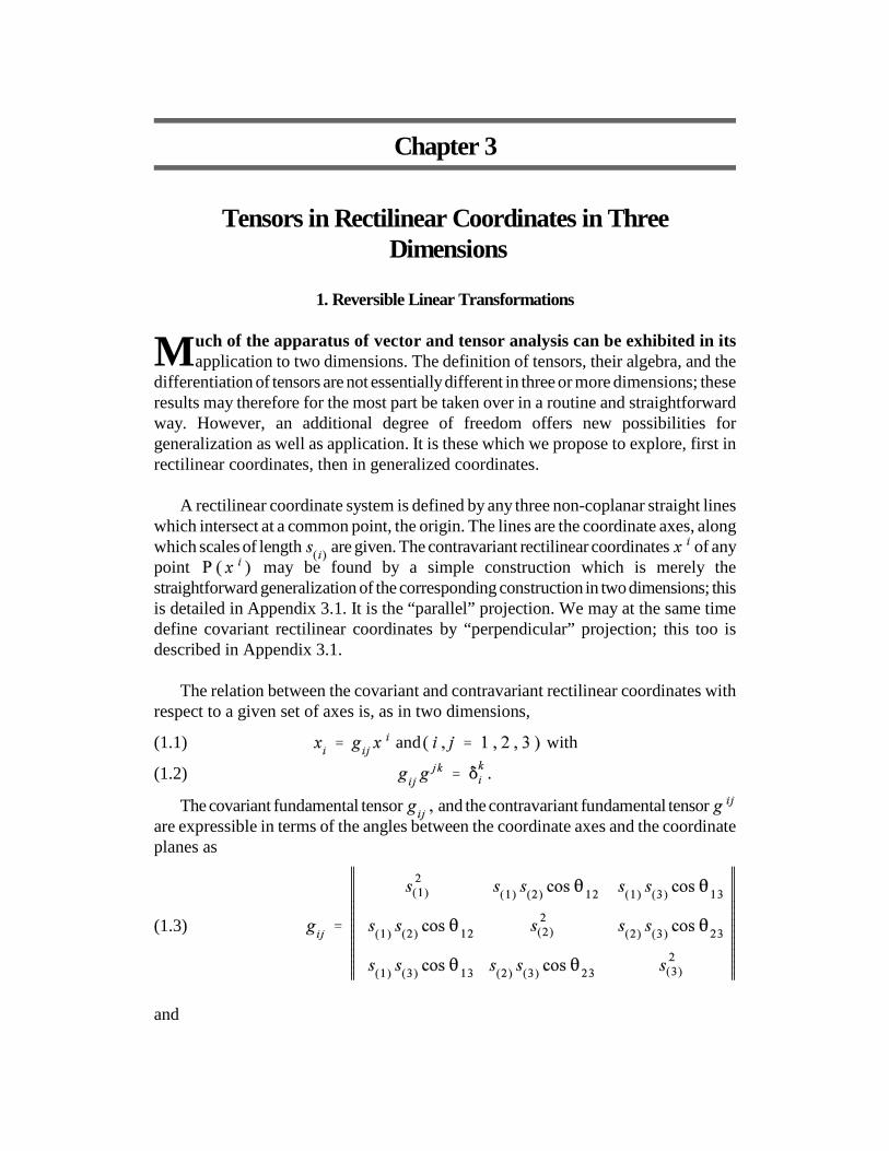
The angles are the dihedral angles along the axes between the respective

planes containing the axes and ( see Fig. 61.)

1. Reversible Linear Transformations 163

We may now consider any two rectilinear coordinate systems with a common originO. The coordinates of a point P may be given in either system. There must therefore bea relation between these two sets of coordinates. It is, predictably, a reversible linearhomogeneous transformation

where the coefficients are, aside from scale factors, known functions of the anglesbetween the three axes (Appendix 3.1, equations (3.1.16)). Conversely, any reversiblelinear homogeneous transformation of rectilinear coordinates may be shown to implya certain change of axes and possibly changes of scale (Appendix 3.2).

We shall henceforth consider these points established and not labor them further.Though the extension to a third dimension has been at the price of a more tediousgeometrical analysis and lengthier formulae, the general argument runs just as it did intwo dimensions. It is to be understood, of course, that in three dimensions indices havethe range 1 to 3. We note, too, that the meaning of the inner product is exactly the samein three dimensions as in two.

Ex. (1.1) (a) Given that

and

find the covariant fundamental tensor in this coordinate system if all the scalefactors are unity. (b) Calculate as the inverse of (c) Check your answersby using equation (1.4).

Ans.

(Hint: )

Ex. (1.2) Given that the rectilinear contravariant coordinates are related tothe Cartesian coordinates by the transformation

what are the components of the fundamental tensor in the new coordinate system?(Hint: ).

Ans.


Ex. (1.3) Determine the inner product of and

Ans.

Ex. (1.4) What is the magnitude of the vector whose components in a Cartesiancoordinate system are

Ans.

Ex. (1.5) Show that we must always have

(Hint: use equation (1.3).)

2. Covariant Vectors, Contravariant Vectors, and Duality

A vector in three dimensions, like a vector in two dimensions, is a set ofcomponents which transform in identically the same way as the rectilinear

coordinates. This implies that a contravariant vector transforms as

and a covariant vector transforms as

when one goes from coordinates to a new system

However, certain distinctions between covariant and contravariant vectors may bebrought out more clearly in three dimensions than in two. For example, consider thevector

It is parallel to the axis since its “parallel” projections upon the other two axes areboth zero. Hence all vectors parallel to the axis are of the form where isan invariant.

Now consider a position vector

It represents a vector in the plane. Hence all vectors in the planeare proportional to some We say that the collection of all such vectors spans the

plane. This plane may also be identified as the two-dimensional sub-space More generally, then, in rectilinear coordinates the sub-space

is spanned by all vectors of the form

Consider next a covariant vector

2. Covariant Vectors, Contravariant Vectors, and Duality 165

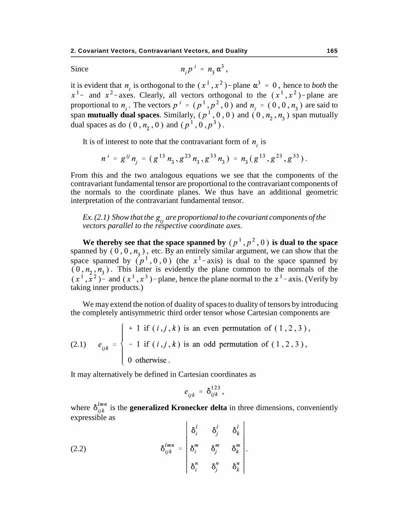
Since

it is evident that is orthogonal to the plane hence to both the and axes. Clearly, all vectors orthogonal to the plane are

proportional to The vectors and are said tospan mutually dual spaces. Similarly, and span mutuallydual spaces as do and

It is of interest to note that the contravariant form of is

From this and the two analogous equations we see that the components of thecontravariant fundamental tensor are proportional to the contravariant components ofthe normals to the coordinate planes. We thus have an additional geometricinterpretation of the contravariant fundamental tensor.

Ex. (2.1) Show that the are proportional to the covariant components of thevectors parallel to the respective coordinate axes.

We thereby see that the space spanned by is dual to the spacespanned by etc. By an entirely similar argument, we can show that thespace spanned by (the axis) is dual to the space spanned by

This latter is evidently the plane common to the normals of the and plane, hence the plane normal to the axis. (Verify by

taking inner products.)

We may extend the notion of duality of spaces to duality of tensors by introducingthe completely antisymmetric third order tensor whose Cartesian components are

(2.1)

It may alternatively be defined in Cartesian coordinates as

where is the generalized Kronecker delta in three dimensions, convenientlyexpressible as

(2.2)


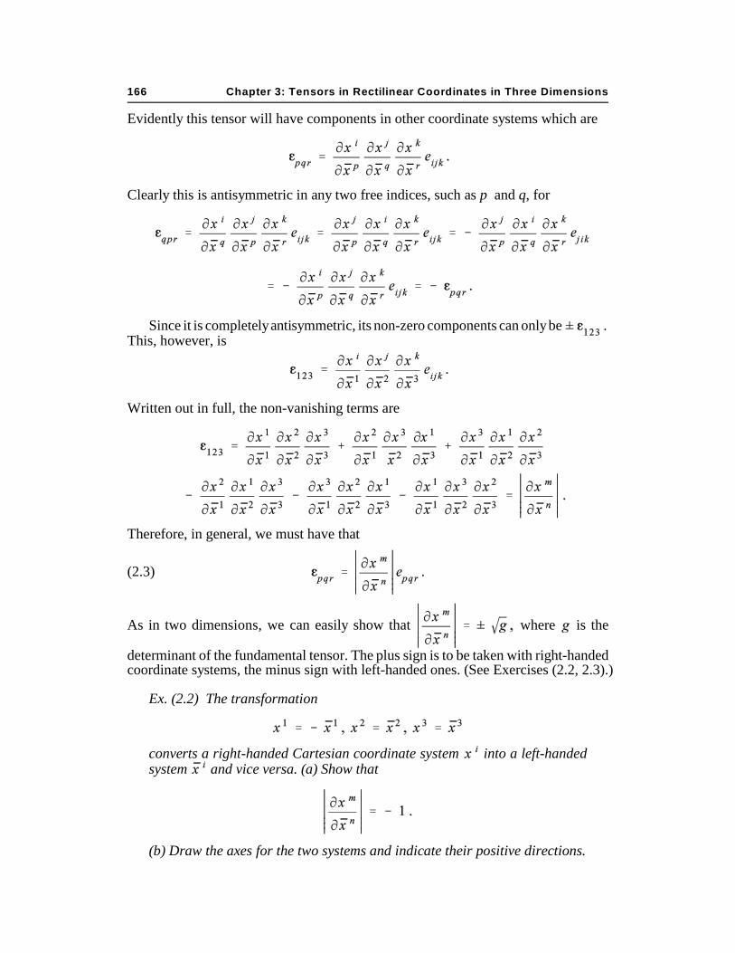
Evidently this tensor will have components in other coordinate systems which are

Clearly this is antisymmetric in any two free indices, such as p and q, for

Since it is completely antisymmetric, its non-zero components can only be This, however, is

Written out in full, the non-vanishing terms are

Therefore, in general, we must have that

(2.3)

As in two dimensions, we can easily show that where is the

determinant of the fundamental tensor. The plus sign is to be taken with right-handedcoordinate systems, the minus sign with left-handed ones. (See Exercises (2.2, 2.3).)

Ex. (2.2) The transformation

converts a right-handed Cartesian coordinate system into a left-handedsystem and vice versa. (a) Show that

(b) Draw the axes for the two systems and indicate their positive directions.


Ex. (2.3) (a) Does the transformation

where the is a right-handed Cartesian system, yield a right-handed or aleft-handed system? (b) What test discriminates between the two?

Ans. (a) Right-handed ; (b) right-handed if

Ex. (2.4) Show that is a completely anti-

symmetric tensor, where

Ex. (2.5) Show that

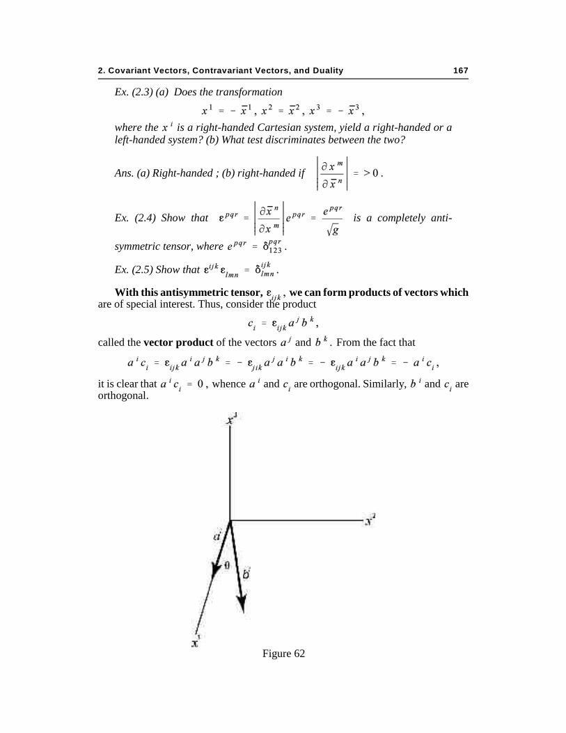
With this antisymmetric tensor, we can form products of vectors whichare of special interest. Thus, consider the product

called the vector product of the vectors and From the fact that

it is clear that whence and are orthogonal. Similarly, and areorthogonal.

Figure 62


We may interpret the vector product of and very readily by evaluating itscomponents in a conveniently chosen coordinate system. We choose for this purpose aCartesian system such that the axis lies along and the axis is perpendicularto it in the plane of and (see Fig. 62). Then

and

(2.4)

From this we see that the vector product of two vectors is perpendicular to both andhas a magnitude equal to the product of their magnitudes times the sine of the anglebetween them. It is also clear that the vector product is the dual to the space spanned bythe two vectors.

Ex. (2.6) In a Cartesian coordinate system, Find the unit vector perpendicular to and

Ans. Since is perpendicular to both

and and since the unit vector in the direction of hascomponents

Since this is a Cartesian system, the components of the contravariant unit normalare the same.

Ex. (2.7) What is the angle between the vectors and of Ex. (2.6)?

Ans. Since and since wehave

To determine the quadrant of we compute

Hence

Ex. (2.8) In a certain oblique coordinate system, the fundamental tensor hascomponents

Find the unit vector perpendicular to and


Ans. Since we have

is perpendicular to and Since the contravariant fundamental tensor is

the magnitude of must be

Therefore, the unit vector perpendicular to and has the covariantcomponents

Ex. (2.9) Show that the inner product of a vector with the vector products ofvectors and is an invariant equal to where

, , and are the magnitudes of and is the angle between and and is the angle between and the plane of and (Hint:Choose a Cartesian coordinate system with the axis along the axisin the plane of and )

Ex. (2.10) Determine the vector product of with that of and

Ans.

More generally, we can say that a tensor

(2.6)

is dual to and conversely. As may be inferred from the examples of duality thus farconsidered, duality implies orthogonality and complementarity both of rank and ofcovariance-contravariance. The reciprocity of this relationship may be furtheremphasized by noting that the vector may be readily recovered from its dual

Thus


Now

since at most only one of the terms of the middle sum can be different from zero.Further,

and and must each be different from two of the values of but the result is in anycase zero unless and are the same. Hence

(2.7)

Ex. (2.11) What is the tensor dual to the covariant vector in three dimensions?(Hint: raise the free indices in equation (2.6) and interchange the summationindices.)

Ans.

Ex. (2.12) Show that in three dimensions. (Hint: use the fact that

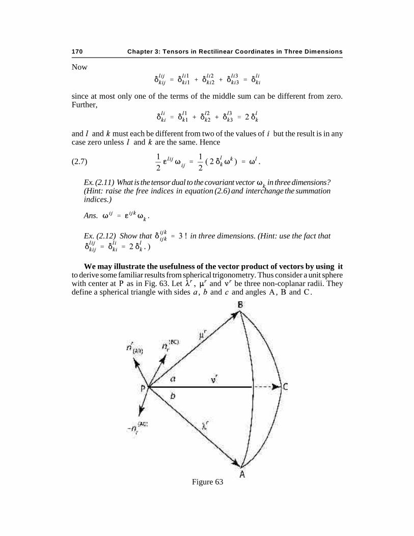
We may illustrate the usefulness of the vector product of vectors by using itto derive some familiar results from spherical trigonometry. Thus consider a unit spherewith center at as in Fig. 63. Let and be three non-coplanar radii. Theydefine a spherical triangle with sides , and and angles , and .

Figure 63


Now consider the invariant

(2.5)

The right-hand side may be written as

inasmuch as all three vectors have unit magnitude.

The left-hand side of equation (2.5), however, may be given the form

where is the unit normal to the plane of and and is the unit normalto the plane of and Therefore the inner product in parenthesis in the precedingexpression is

Equating the values thus found for the two sides of the original equation, we then have

or

the law of cosines of spherical trigonometry.

Next, let us consider the invariant

Since

we must have

where is the unit normal to the plane of and Now because

is normal to both normals, it must lie in both the planes of and as well as of and hence be along their intersection. That is, we must have

The invariant thus has the value


On the other hand, we may express also in the form

Therefore

By permuting and on the right hand side, we get expressions which areunchanged except for the order of the terms. On the other hand, two new expressions aregenerated on the left. Hence

In the form

this is the law of sines of spherical trigonometry.

Figure 64

3. Points, Lines, and Planes 173

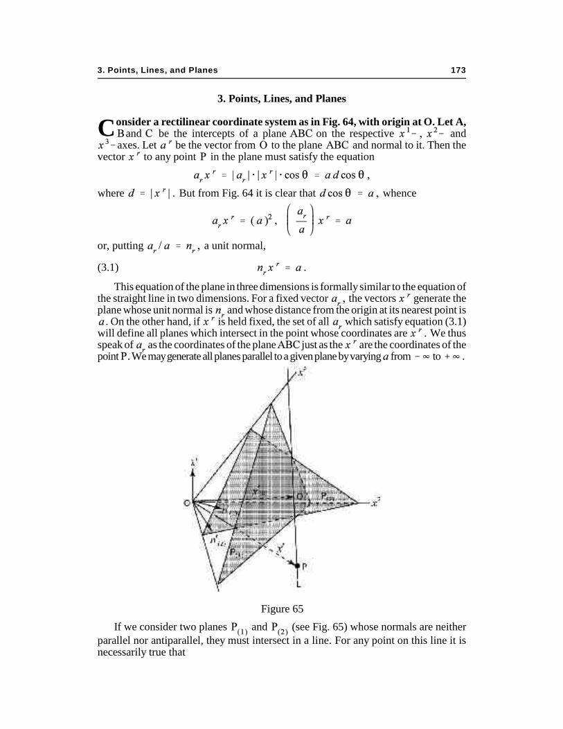
Figure 65

3. Points, Lines, and Planes

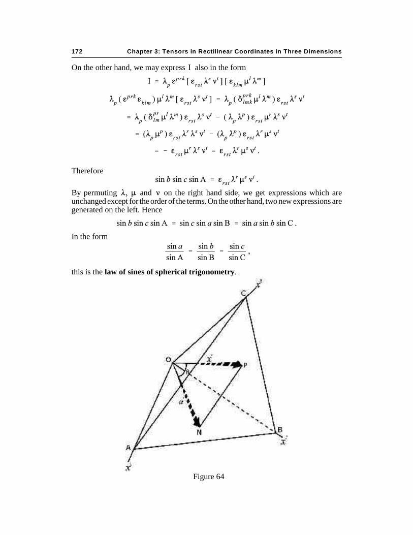
Consider a rectilinear coordinate system as in Fig. 64, with origin at O. Let A,and be the intercepts of a plane on the respective and

axes. Let be the vector from to the plane and normal to it. Then thevector to any point in the plane must satisfy the equation

where But from Fig. 64 it is clear that whence

or, putting a unit normal,

(3.1)

This equation of the plane in three dimensions is formally similar to the equation ofthe straight line in two dimensions. For a fixed vector the vectors generate theplane whose unit normal is and whose distance from the origin at its nearest point is

. On the other hand, if is held fixed, the set of all which satisfy equation (3.1)will define all planes which intersect in the point whose coordinates are We thusspeak of as the coordinates of the plane just as the are the coordinates of thepoint . We may generate all planes parallel to a given plane by varying from to

If we consider two planes and (see Fig. 65) whose normals are neither

parallel nor antiparallel, they must intersect in a line. For any point on this line it isnecessarily true that


(3.2)

These are two linear equations in three unknowns. They therefore imply that in generala one-parameter linear relation must exist among common coordinates (components)

Without loss of generality, we may suppose this relation to be of the parametricform

(3.3)

where is a unit vector and is the parameter. Now the vector corresponding to the value of the parameter, must satisfy the equations

(3.2). Hence

(3.4)

Therefore, multiplying equation (3.3) by and using equations (3.2) and (3.4),

we see that or and are orthogonal. In a similar way, we can show

that and are orthogonal. Therefore

(3.5)

Let us now multiply both sides of equation (3.3) by This gives

If we choose to be the point on the line nearest the origin, then

(3.6)

and is simply the distance from along the line. We see also that isorthogonal to

Ex. (3.1) (a) Identify the plane whose equation is

in a Cartesian coordinate system. (b) Do the same for the plane whose equationis

(c) find the equation of the line in which they intersect. (Hint: is a solution ofequations (3.2) and (3.6).)

Ans. (a) The vector has magnitude Hencethe equation of the plane in canonical form is

3. Points, Lines, and Planes 175

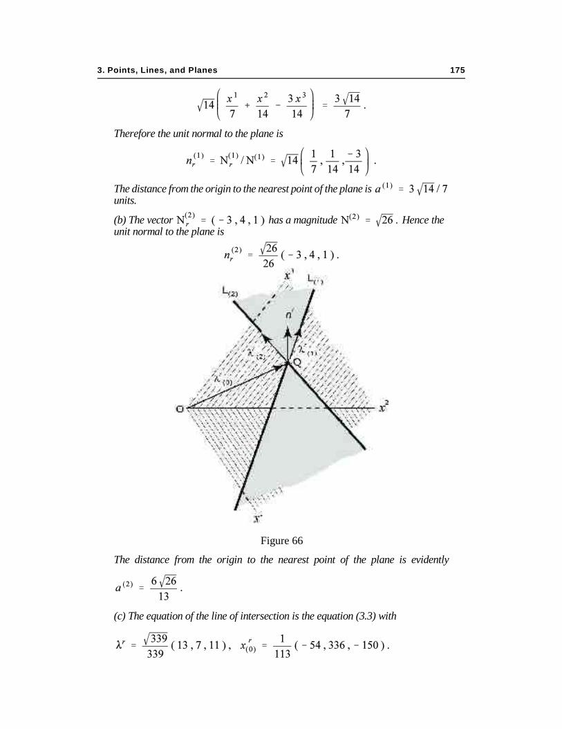
Figure 66

Therefore the unit normal to the plane is

The distance from the origin to the nearest point of the plane is units. (b) The vector has a magnitude Hence the unit normal to the plane is

The distance from the origin to the nearest point of the plane is evidently

(c) The equation of the line of intersection is the equation (3.3) with


We have seen how to determine the equation of the line which is formed bythe intersection of two planes. Let us now consider the converse problem: What is theplane containing two given intersecting straight lines? We suppose the lines to have theequations

(3.7)

where the are the components of the position vector to any point on the line, and are the respective parameters of the lines, and are the position vectors of a

particular point on the line (conveniently the point nearest the origin), and and the unit vectors in the directions of the lines. To be certain that the two lines are notidentical or parallel, we require that

Suppose that is the position vector to the point of intersection of the two lines.Then clearly if is in the plane containing the two lines, must be some

linear combination of and Hence

(3.8)

is the equation of this plane. The two arbitrary parameters and are the parametersof the plane.

To put this equation for the plane into the form of equation (3.1), we first form theunit normal

(3.9)

Multiplying equation (3.8) through by we see that

This is the desired result.

Ex. (3.2) Show that the plane defined by two lines whose equations are given inequation (3.7) could equally well have equations of the form

Thus, show that the condition for the intersection of the two lines is that

(Hint: Both and must lie in the plane and and will in any casespan the plane.)

4. Cones and Quadrics 177

4. Cones and Quadrics

We have seen that in general, an equation of the form

is the equation of a straight line in rectilinear coordinates in two dimensions; in threedimensions it is more generally the equation of a plane. We have also seen that in twodimensions, an equation of the form

is in general the equation of an ellipse or hyperbola or a pair of straight linesWe now inquire what such an equation represents in three dimensions.

First, we recognize that there is no loss of generality in supposing that is

symmetric, for if it is not, it may be resolved as

into a symmetric part and an antisymmetric part Then

But

hence it is zero.

We therefore proceed by asking the question: Is there some vector or vectors suchthat, given a symmetric tensor there is a constant such that

If so, we must have

a set of equations whose only solution is unless

(4.1)

Expanded, this equation gives a cubic in namely


Since the coefficients of the powers of are all invariants, the roots of this equationmust be also. We know that at least one root must be real inasmuch as every cubicpolynomial with real coefficients must have at least one real root.

Let us write equation (4.1) in the form

We can now show that not only are the roots of the determinantal equationinvariants, but all are real if is symmetric. To do so, suppose that one of the roots

is complex. Then it would be true that

for some necessarily complex eigenvector That is,

Therefore

(4.2)

Multiplying the former by the latter by and subtracting, we get

Since not both and can be zero, it follows that whence isreal. Note that this proof is independent of the fact that the number of dimensions isthree.

We may note also, for the sake of future applications (as to moment of inertiatensors), that if for all non-zero then from equation (4.2),multiplying the first by and the second by and subtracting, we get

Since both the left hand side and the parenthesis on the right hand side are positive, soalso is . In this case, the roots are not only real invariants, but positive as well. When satisfies the condition for all non-zero it is said to be positivedefinite.

We have therefore shown that the equation

(4.3)

4. Cones and Quadrics 179

has a solution for three values of the eigenvalues. These solutions

are the eigenvectors. As before, we can show that theseeigenvectors are mutually orthogonal if the eigenvalues are distinct. Thus

But because

Since we postulated that it follows that The

eigenvectors are therefore orthogonal.

Ex. (4.1) Find the eigenvalues and the eigenvectors of the symmetric tensor

where the fraction multiplies each component within the matrix. Take thecoordinate system to be Cartesian.

Ans. The determinantal equation is

The roots of this equation are When the solution of theequation is

arbitrary. The other eigenvectors are

Ex. (4.2) Show that the eigenvectors of Ex. (4.1) are mutually orthogonal.

This being the case, we may adopt the directions of the eigenvectors, theinvariant directions, as the directions of a set of orthogonal axes. In this referencesystem we have

By substitution of these vectors into equation (4.3), we can show at once that

Chapter 3. Tensors in Rectilinear Coordinates in Three Dimensions180

where because the coordinate axes are orthogonal. In other words, thesymmetric tensor becomes a diagonal tensor in the reference frame of the invariantdirections.

It is now very easy to see what the equation

(4.4)

represents. In the frame of reference of the invariant directions, it is simply

where The position vectors which satisfy this

equation evidently define a quadric provided not all are negative. The semi-axes ofthe quadric are equal to

If but the are not all of the same sign, then clearly equation (4.4) is that

of a cone. If the are all of the same sign, the equation (4.4) can be satisfied only by

Ex. (4.3) Interpret the equation

where has the Cartesian components given in Ex. (4.1).

Ans. This equation represents an ellipsoid with axes and along the directions of the eigenvectors.

5. The Kinematics of Rigid Bodies

Aprincipal application of vectors and tensors in rectilinear coordinates is tothe motion of rigid bodies. We define a rigid body as a set of particles whose

mutual distances are fixed. Where such a conception need be made more refined,summation over particles may be replaced by integration over mass elements. With noessential loss of generality, however, we may treat the dynamics of rigid bodies as thatof a set of rigidly connected particles.

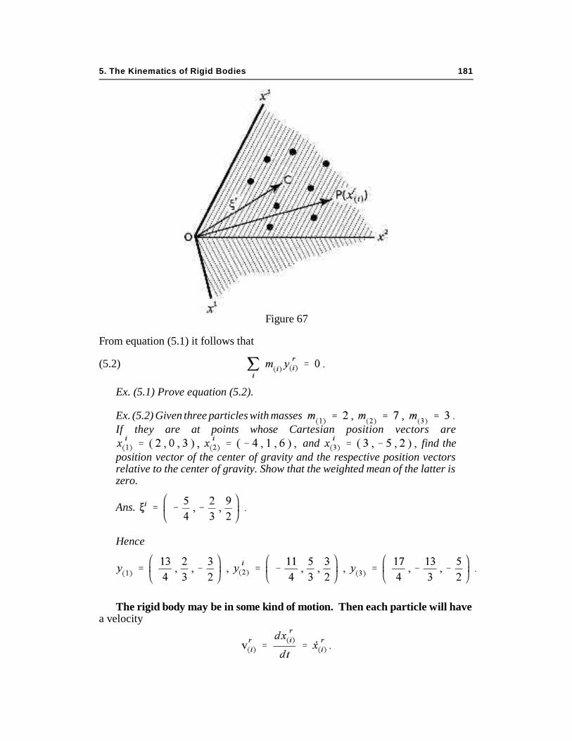
Let be a set of rectilinear coordinates in an inertial frame of reference. Let theparticle of mass have coordinates that is, let the particle have aposition vector whose components are We now define the center of gravity of theset of particles (see Fig. 67) to be the point C whose position vector is given by

(5.1)

With respect to the center of gravity, the ith particle has a position vector

5. The Kinematics of Rigid Bodies 181

From equation (5.1) it follows that

(5.2)

Ex. (5.1) Prove equation (5.2).

Ex. (5.2) Given three particles with masses If they are at points whose Cartesian position vectors are

and find theposition vector of the center of gravity and the respective position vectorsrelative to the center of gravity. Show that the weighted mean of the latter iszero.

Ans.

Hence

The rigid body may be in some kind of motion. Then each particle will havea velocity

Figure 67


The velocity of the center of gravity will be With respect to the center of gravity, thevelocity of each particle will be

From equation (5.2) it is clear that

(5.3)

Between any two particles and there is a fixed distance

Since this is a constant distance within a rigid body, its time derivative is zero, whence

(5.4)

But clearly

which implies that

Therefore equation (5.4) becomes

or

(5.5)

for all and . Now for fixed let this equation be multiplied by and summedover . The result will be

By equations (5.2) and (5.3), the sums on the right hand side are zero. Hence

(5.6)


Multiply this equation by and sum over . We then have

Since this is to be true whatever values may be assigned the it follows that

(5.7)

for each . This implies that the left hand side of equation (5.5) vanishes, whence fromthe right hand side

(5.8)

for all and .

Let us note in passing that from equation (5.7) we can infer also that

This implies that the distance of particle from the center of gravity does notchange; i.e., the center of gravity is at a fixed point within the rigid body.

Let us now examine equation (5.8), which we write as

Now for any this must be true for every , and vice versa. Hence must be a linearhomogeneous function of the same linear function that is of That is, wemust have

(5.9)

where is a covariant second rank tensor. Substituting equation (5.9) into equation

(5.8), it becomes

(5.10)

In general, this requires that

(5.11)

Hence is an antisymmetric covariant tensor of the second rank. It is called theangular velocity tensor.


The dual of the angular velocity tensor is the angular velocity vector

(5.12) whence

To give a geometrical interpretation, we consider a point within the rigid bodywhose position vector has components where is some convenientinvariant parameter. Then by equation (5.9), the velocity of the particle at point is

In other words, the line defined by the equation lying along is at restrelative to the center of gravity. It is called the instantaneous axis of rotation. Themagnitude of is called the angular velocity.

We note finally that when we must also have Then

for all . Such a motion is called a pure translation.

Ex. (5.3) Given an angular velocity vector whose Cartesian components are (a) What is the magnitude of the angular velocity vector?

(This is usually termed simply the angular velocity.) (b) What angles does it makewith the coordinate axes? (c) What are the components of the angular velocitytensor?

Ans. (a) The units are angle per unit time. Most commonly, this isradians/second, or some similar unit. (b) Since

where the quantities in parentheses are the components of a unit vector, we have

Ex. (5.4) If is the angular velocity vector, then all vectors which satisfy thecondition

(5.13)


define the plane of the equator of the rigid body. Since satisfies thisequation, it is clear that the center of gravity lies in the plane of the equator. Theequation also indicates that the equator and the axis of rotation are mutuallyorthogonal.

Show that for any point in the plane of the equator the angular velocity tensoris given by the expression

(5.14)

Ans. Since it is clear that and are

orthogonal. By equation (5.13), and are likewise. Hence and form an orthogonal triad, so that

(5.15)

where is an invariant factor to be determined. The value of may be fixed bynoting that

Since we may take this as a true equation by choosing

whence equation (5.14) follows from equations (5.12) and (5.15).

Ex. (5.5) Show that the axis of rotation is defined by the location of any two pointson the equator which are not collinear with the center of gravity.

Ans. If the two points are and then

and

provide two independent equations from which the ratios may befound provided constant.

Ex. (5.6) Given that in a Cartesian coordinate system at time (a)

Find the

position vector of the center of gravity. (b) If the particles have respective velocities

and find the

velocity of the center of gravity. (c) What are the particles’ position vectors relativeto the center of gravity? (d) What are the particles’ velocities relative to the centerof gravity? (e) What is the angular velocity tensor of the system? (Hint: useequation (5.14).) (f) What is the angular velocity vector for the system? (Useequation (5.12).) (g) Check your answer to (f) by using equation (5.15).


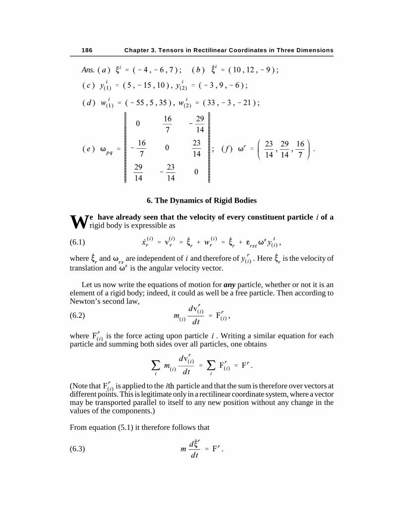
Ans.

6. The Dynamics of Rigid Bodies

We have already seen that the velocity of every constituent particle of arigid body is expressible as

(6.1)

where and are independent of and therefore of Here is the velocity oftranslation and is the angular velocity vector.

Let us now write the equations of motion for any particle, whether or not it is anelement of a rigid body; indeed, it could as well be a free particle. Then according toNewton’s second law,

(6.2)

where is the force acting upon particle . Writing a similar equation for eachparticle and summing both sides over all particles, one obtains

(Note that is applied to the particle and that the sum is therefore over vectors atdifferent points. This is legitimate only in a rectilinear coordinate system, where a vectormay be transported parallel to itself to any new position without any change in thevalues of the components.)

From equation (5.1) it therefore follows that

(6.3)

6. The Dynamics of Rigid Bodies 187

In other words, the center of gravity of a system of particles — any system — movesas though it were a particle of the same total mass as the system, acted upon by a netforce equal to the total sum of all the forces, applied at the center of gravity. Since rigidbodies have not been excluded, this is true of rigid bodies as well as any other systemof particles.

Let us now multiply both sides of equation (6.2) by and sum over .Then, again for any system of particles,

Now since

the preceding equation may be written in the form

(6.4)

The quantity

(6.5)

is called the angular momentum of the system of particles. The quantity

(6.6)

is called the moment of the system of forces, or the torque. The equation ofmotion of the system is therefore

(6.7)

Ex. (6.1) (a) Calculate the instantaneous angular momentum of the system inEx. (5.6). (b) Calculate the instantaneous moment of the forces, given that

Ans.


The equations (6.3) and (6.7) are the equations of motion of the system ofparticles, whether constituting a rigid body or not. Let us now further specialize theequations to the case of a rigid body. The first equation requires no modification, for itgoverns the motion of a point, the center of gravity. To particularize equation (6.7),however, we substitute equation (6.1) into equation (6.5), obtaining

The first term on the right hand side is the angular momentum of the center of gravitywith respect to the origin. The second and third terms vanish, by equation (5.2). Inconsidering the final term, we first define the quantity

(6.8)

called the inertia tensor of the system about the center of gravity. In terms of this, thelast term becomes

where

(6.9)

is called the inertia invariant.

We thus have, after lowering indices, that

(6.10)

where

(6.11)

Equations (6.7), (6.8), (6.9), and (6.10) now describe the motion of a rigid body.

6. The Dynamics of Rigid Bodies 189

As a next step, we may re-fashion the expression (6.6) for the moment of forces.Thus

(6.12)

where

(6.13)

is the moment of forces about the center of gravity. The equation of motion (6.7) for a rigid body now becomes

Equating the middle terms and using equation (6.2), we see that the equation of motionfinally reduces to

(6.14)

We thus see that not only does the center of gravity move as would a free particle of thesame total mass, subject to the same set of forces, but at the same time the body movesrelative to the center of gravity as though the center of gravity were at rest and the bodywere subjected to the action of the same forces.

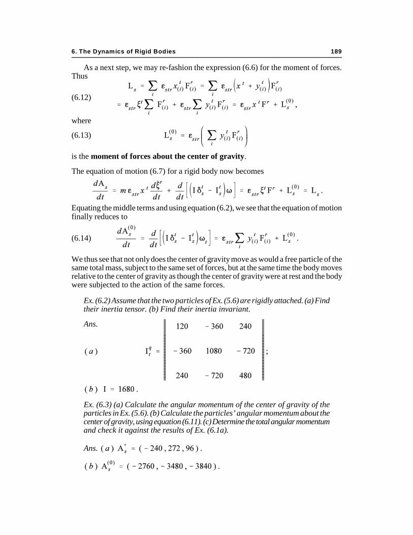
Ex. (6.2) Assume that the two particles of Ex. (5.6) are rigidly attached. (a) Findtheir inertia tensor. (b) Find their inertia invariant.

Ans.

Ex. (6.3) (a) Calculate the angular momentum of the center of gravity of theparticles in Ex. (5.6). (b) Calculate the particles’ angular momentum about thecenter of gravity, using equation (6.11). (c) Determine the total angular momentumand check it against the results of Ex. (6.1a).

Ans.


7. Rotating Axes

In making use of the equations of motion of a rigid body, it is clear that therewill in general occur time derivatives of the inertia tensor and the inertia invariant.

Since the inertia tensor characterizes a rigid body, it should be possible to avoid anyconsideration of the derivatives of the inertia tensor by transforming to moving axeswith respect to which the moments of inertia are constant in time.

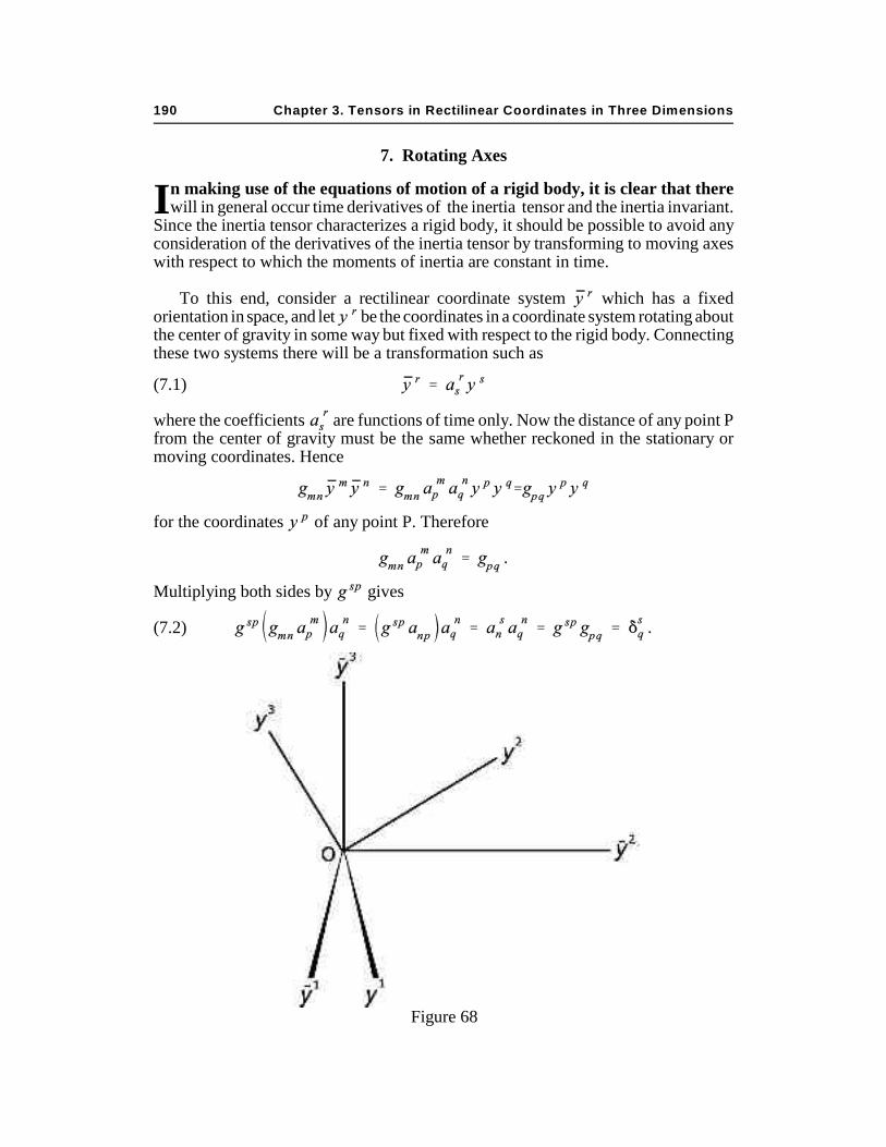
To this end, consider a rectilinear coordinate system which has a fixedorientation in space, and let be the coordinates in a coordinate system rotating aboutthe center of gravity in some way but fixed with respect to the rigid body. Connectingthese two systems there will be a transformation such as

(7.1)

where the coefficients are functions of time only. Now the distance of any point Pfrom the center of gravity must be the same whether reckoned in the stationary ormoving coordinates. Hence

for the coordinates of any point P. Therefore

Multiplying both sides by gives

(7.2)

Figure 68

7. Rotating Axes 191

From this we see, by taking determinants of both sides, that

Hence but since the transformation is a continuous one and we may,without loss of generality, take the initial value of to be we see that the plus signholds. It is easy to show also that the are, in fact, the cosines of the angles whicheach of the axes makes at any instant with the respective axes. (See Appendix 3.2).

A further condition upon the may be derived by considering a point which

is fixed in the rotating system. Then Consequently, when we differentiateequation (7.1) we get

(7.3)

Since we must also have that

equation (7.3) becomes

Multiply this by then

But from equation (7.2) it follows that

Therefore, for any or

whence

(7.4)

We may make use of this result in finding the derivative of the angular momentum.Thus, from equation (7.2) we have that is its own inverse, so that the vectortransformation from to requires that


Now the equation of motion about the center of gravity is

so that the right hand side of the preceding equation is

The final form of the equation in the coordinates therefore becomes

(7.5)

This is therefore the equation of motion of a rigid body in a system of coordinates withorigin at the center of gravity and rotating axes fixed in the body itself.

Let us consider further the inertia tensor From its definition as

it is clear that is symmetric in and . Moreover, it is clear that

it is therefore a positive definite form. As we have seen, this implies that the roots of thedeterminantal equation

are both real and positive. There is therefore a transformation which will reduce tothe diagonal form

(7.6)

8. Strain 193

with Moreover, the coordinate system in which has the form of equation

(7.6) is an orthogonal system with axes in the invariant directions. This is called aprincipal-axis coordinate system.

If a principal-axis coordinate system is used, we will have for the angularmomentum

Equation (7.5) therefore becomes

(7.7)

At first glance, the second term on the left hand side of equation (7.7) may appear

to be zero because of the term However, closer inspection shows that thisis in general not the case because of the factor Let us write out thecomponents of this term explicitly; they are

It is apparent, therefore, that equation (7.7) may be given the final form

(7.8)

In practice, this is a somewhat more convenient and useful form than Eq. (7.5).

Ex. (7.1) Show without writing out the terms that does not vanish

identically if (Hint: use the fact that in general ) Ex. (7.2) Show that

(Hint: use the result of Ex. (7.1).) Ex. (7.3) From Appendix (3.1) show that

hence that

8. Strain

The motion of rigid bodies has been analyzed by considering those motionsunder which the mutual distances of particles or mass elements remain constant. If

this condition be waived, the matter constitutes an elastic medium or fluid. Let us seehow such a medium may be described.


Again, let be the position vector of a mass element. The distance between anytwo elements and is then

Suppose each element to be continuously displaced during a small time interval .Then the separation of elemenmattts and changes at a rate

(8.1)

Now if both mass elements are near the origin and if is small, then to a firstapproximation (by a Maclaurin series, for example)

(8.2) ,

terms of higher order being neglected. Here is taken to be independent of solong as is small, there is no loss of generality in this assumption.

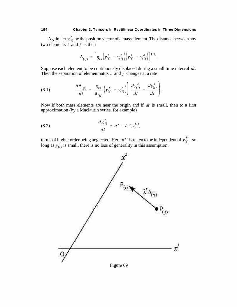
Figure 69

8. Strain 195

The vector clearly contributes nothing to the right hand side of equation (8.1);it corresponds to a pure translation. To assess the contribution of we resolve it intosymmetric and antisymmetric parts; thus

(8.3)

Then

The last term vanishes inasmuch as is antisymmetric in and ; it corresponds toa pure rigid rotation.

Both translation and rotation are rigid body displacements. The sole remaining term,the only one making a non-zero contribution to the variation of the separation of theelements and , is

(8.4)

The symmetric tensor is called the rate of strain tensor. It fully characterizes themanner in which the medium has been distorted at each point.

To interpret the strain tensor, consider two points and (Fig. 69) betweenwhich the vector is initially

where is clearly a unit vector in the direction from to Then the strain will be such that the points and separate at a rate

In other words, the distance between elements and increases in proportion to theinitial distance between them and to Since the unit vector may be inany direction whatever, depending on the identity of the elements, it is clear that completely characterizes the distortion of the medium in the neighborhood of everypoint. Thus, to specify a distortion is to determine a strain tensor and vice versa.


Figure 70

Appendix 3.1 : The Transformation to New Axes and New Units of Length

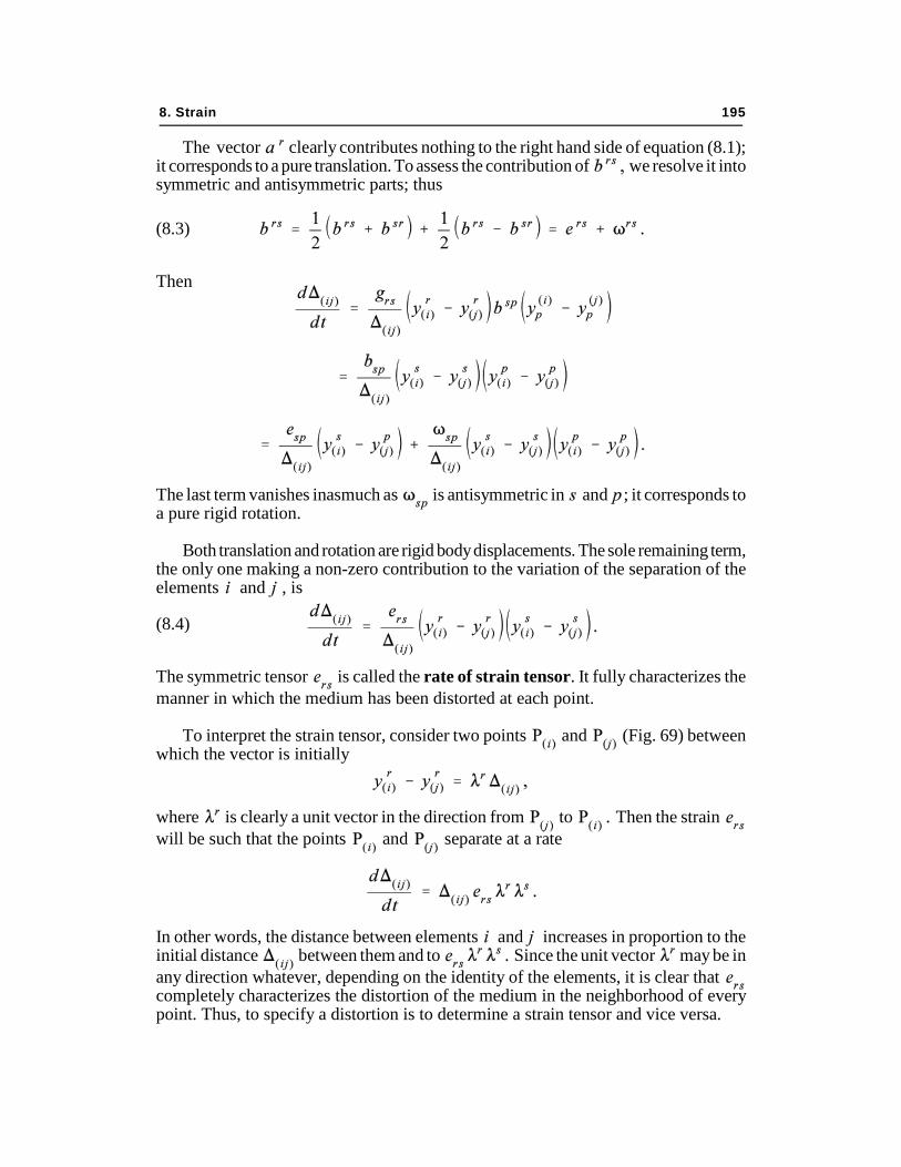
Consider three planes which mutually intersect by pairs and have the singlepoint in common. We take the point as the origin (see Fig. 70). Let the

intersections of the planes be the lines They will serve ascoordinate axes. Through any point draw a line parallel to . Point is the

intersection of this line with the plane of and . Through draw a lineparallel to . This line intersects the axis at . Then by definition, therectilinear contravariant coordinates of the point are

At the same time, we project onto If theperpendicular onto intercepts the length then the covariant rectilinearcoordinate is in this system of axes. Projections onto the other axes givethe other covariant rectilinear coordinates.

Now the projection of any continuous set of line segments beginning at andending at is the same as the projection of itself. Thus the projection of the jointedcurve is the same as the projection of upon the same axes; it is the sum ofthe projections of and

Appendix 3.1: The Transformation to New Axes and New Units of Length 197

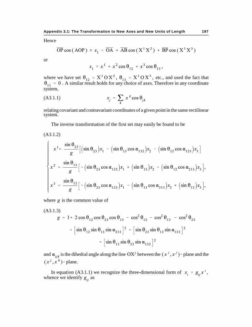
Hence

or

where we have set etc., and used the fact that A similar result holds for any choice of axes. Therefore in any coordinate

system,

(A3.1.1)

relating covariant and contravariant coordinates of a given point in the same rectilinearsystem.

The inverse transformation of the first set may easily be found to be

(A3.1.2)

where is the common value of

(A3.1.3)

and is the dihedral angle along the line between the plane and the

plane.

In equation (A3.1.1) we recognize the three-dimensional form of whence we identify as


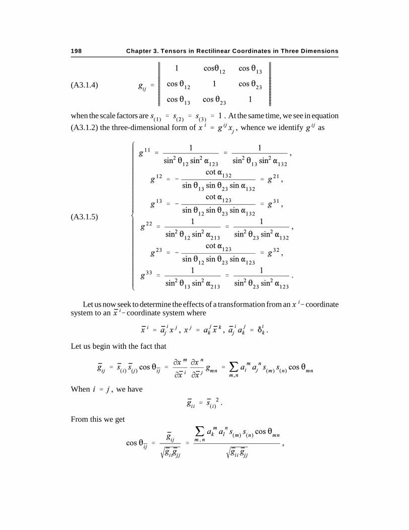
(A3.1.4)

when the scale factors are At the same time, we see in equation

(A3.1.2) the three-dimensional form of whence we identify as

(A3.1.5)

Let us now seek to determine the effects of a transformation from an coordinatesystem to an coordinate system where

Let us begin with the fact that

When we have

From this we get

Appendix 3.1: The Transformation to New Axes and New Units of Length 199

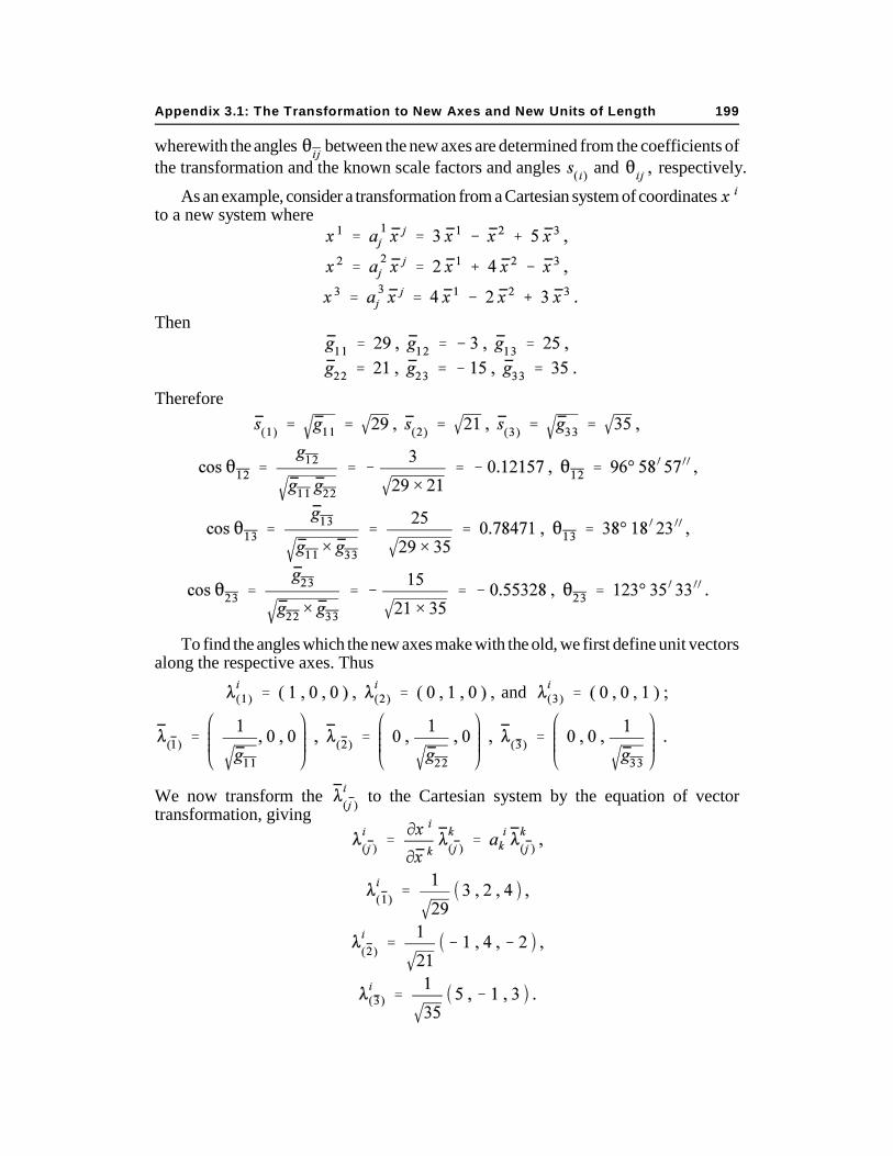
wherewith the angles between the new axes are determined from the coefficients ofthe transformation and the known scale factors and angles and respectively.

As an example, consider a transformation from a Cartesian system of coordinates to a new system where

Then

Therefore

To find the angles which the new axes make with the old, we first define unit vectorsalong the respective axes. Thus

and

We now transform the to the Cartesian system by the equation of vectortransformation, giving


The angle between these unit vectors and those along the Cartesian axes is

Hence

The angles between the other axes could be determined in a similar way, but the resultswould be redundant inasmuch as the three scale factors and six angles completelydetermine the relation of the two cordinate systems.

Appendix 3.2: Interpretation of the Transformation to Rotating Axes

We may readily interpret the coefficients of by considering what operationthe tensor performs upon a unit vector along an axis. Thus, let

be such a unit vector along the axis. Then the vector

is one whose components are

Let us form the inner product of with

Then

where is the angle between and If we now require that also be a unitvector, we see that

We have only to adopt the as a unit vector along the axes to see that thetransformation (7.1) converts the axes into the axes. Therefore the are thecosines of the angles between the two sets of axes, hence symmetric.

Notes — Chapter 3 201

Notes — Chapter 3

§3.3. For a more extensive treatment of points, lines and planes, see McConnell (9), Chs.IV and V.

§3.4. For a more extensive treatment of cones and quadrics, see McConnell (9), Chs. VI— IX.

§§3.5 — 3.7. Many common problems concerning systems of particles and themechanics of rigid bodies are considered in detail in Spiegel (16), Chs. 7 to 10.

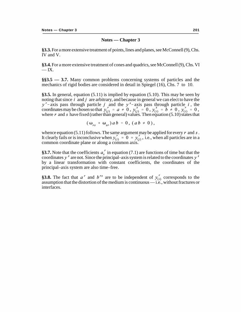
§3.5. In general, equation (5.11) is implied by equation (5.10). This may be seen bynoting that since and are arbitrary, and because in general we can elect to have the

axis pass through particle and the axis pass through particle , thecoordinates may be chosen so that where and have fixed (rather than general) values. Then equation (5.10) states that

whence equation (5.11) follows. The same argument may be applied for every and .It clearly fails or is inconclusive when i.e., when all particles are in acommon coordinate plane or along a common axis.

§3.7. Note that the coefficients in equation (7.1) are functions of time but that thecoordinates are not. Since the principal–axis system is related to the coordinates by a linear transformation with constant coefficients, the coordinates of theprincipal–axis system are also time–free.

§3.8. The fact that and are to be independent of corresponds to theassumption that the distortion of the medium is continuous — i.e., without fractures orinterfaces.

Chapter 3 Tensors in Rectilinear Coordinates in Three Dimensions · 2018-09-09 · Chapter 3...

Documents

Transcript of Chapter 3 Tensors in Rectilinear Coordinates in Three Dimensions · 2018-09-09 · Chapter 3...