Chapter 3 Stream Discharge - Missouri … Discharge 12/09 Introductory Level Notebook 1 Chapter 3...

Stream Discharge 12/09 Introductory Level Notebook 1

Chapter 3

Stream Discharge

- Introductory Level Volunteer Water Quality Monitoring Training Notebook -

What is Discharge (Flow)?

Discharge, also called flow, is the amount of water that flows past a given point in a

given amount of time. Flow is the product of the cross-sectional area multiplied by the

velocity. The rate of discharge is expressed as cubic feet per second (“cfs” or “ft3/sec”).

Discharge Affects the Water Quality of a Stream in a Number of Ways:

Concentrations of Pollutants and Natural Substances – In larger volumes of

faster-moving water, a pollutant will be more diluted and flushed out more quickly than an

equal amount of pollutant in a smaller volume of slower-moving water.

Oxygen and Temperature – Higher volumes of faster-moving water churn

atmospheric oxygen into the water. Smaller volumes of slower-moving water can heat up

dramatically in the summer sun. Remember that hot water holds less dissolved oxygen than

cold water.

Physical Features – Stream discharge interacts with the gradient and substrate of a

stream to determine the types of habitats present, the shape of the channel and the

composition of the stream bottom.

Transport of Sediment and Debris – A larger volume of fast-moving water carries

more sediment and larger debris than a small volume of slow-moving water. High volume

discharges have greater erosional energy, while smaller and slower discharges allow

sediment to settle out and be deposited. These alternating erosional and depositional cycles

determine stream channel shape and sinuosity (i.e., how much the stream channel curves

back and forth).

Plants and Animals Present – Discharge affects the chemical and physical nature of

streams and thus determines what can live there. Fish like salmonids (trout and salmon) and


pollution-sensitive macroinvertebrates require high concentrations of dissolved oxygen, low

water temperatures and gravel substrates for egg laying. Fish such as carp and catfish and

pollution-tolerant macroinvertebrates can survive in warmer water and softer substrates.

Biological Cues – Specific flow volumes and velocities contribute to a group of cues

that combine to trigger spawning in many species of aquatic life.

Minimum Instream Flow – These are requirements for streams subject to

withdrawals of water for domestic water use, hydropower generation and irrigation.

Withdrawals may leave little water for fish and other aquatic life at crucial stages of their

lives. Minimum instream flows can be established to maintain fish populations and to

balance competing out-of-stream uses.

Discharge impacts everything from the concentration of substances dissolved in the

water to the distribution of habitats and organisms throughout the stream!!

Factors Affecting the Volume of Flow

Precipitation is the primary factor because it usually provides the greatest percent of

water for streams. After a rainstorm, stream flow follows a predictable pattern where it rises

and then falls in the hours and days following the storm.

Base Flow is the sustained portion of stream discharge that is drawn from natural

storage sources such as groundwater and not affected by human activity or regulation.

Vegetation along the banks and within the floodplain absorbs water then releases it to

the air through evapotranspiration while deep roots increase the water storage capacity of

soil. In these ways, vegetation will influence the volume of water reaching the water table

and stream, and water availability year round.

Shallow Groundwater, Springs, Lakes, Adjacent Wetlands and Tributaries all

may contribute portions of the total flow in a stream and can be crucial during dry times.


Factors Affecting the Velocity of Flow

Gradient is a key factor. The steeper the gradient (or slope), the faster the water

flows. The gradient of a stream is expressed as the vertical drop of a stream over a fixed

distance, like 1 foot per mile. On a topographical map, contour lines crossing the stream

indicate elevation change. The map scale establishes distance.

Resistance is another key factor. Resistance, also referred to as roughness, is

determined by the nature of the substrate, channel shape, instream vegetation and the

presence of woody debris such as logs and root wads. The unevenness of streambed material

and vegetation contributes resistance to stream flow and slows the water velocity by causing

friction.

Human Activities That Affect Flow

Land-Use – When vegetated areas and wetlands are converted to bare soil and/or

impervious surfaces the volume and velocity of runoff increases dramatically during storm

events. Impervious surfaces include any surface that impedes the infiltration of water, such

as streets, parking lots or rooftops. Therefore, during wet periods, a loss of vegetation and

wetlands results in an excess volume of water runoff that moves at a higher velocity, and are

referred to as “flashy streams.” In dry times, however, the opposite problem occurs.

Without natural vegetation or wetlands, much of the water storage capacity of a watershed is

lost. In dry times, stream flow may be severely reduced or even non-existent.

Channelization – The straightening of a channel and removal of woody debris and

other large objects increases the velocity of flow by increasing the gradient within that reach.

This can vastly increase erosion within the stream, and can increase flooding downstream

from the channelized area. However, streams naturally prefer to meander and if left alone,

will slowly regain sinuosity.

Dams – Dams change the flow of water by slowing or detaining it. The rate at which

hydroelectric dams release water fluctuates greatly in both timing and volume causing large

variances in stream flows. This can dramatically alter the physical and chemical conditions

in streams, both upstream and downstream of the dam.


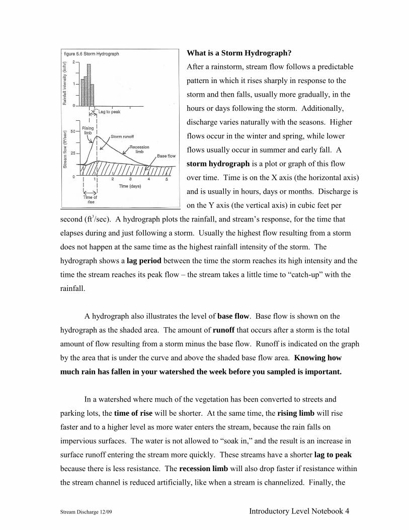
What is a Storm Hydrograph?

After a rainstorm, stream flow follows a predictable

pattern in which it rises sharply in response to the

storm and then falls, usually more gradually, in the

hours or days following the storm. Additionally,

discharge varies naturally with the seasons. Higher

flows occur in the winter and spring, while lower

flows usually occur in summer and early fall. A

storm hydrograph is a plot or graph of this flow

over time. Time is on the X axis (the horizontal axis)

and is usually in hours, days or months. Discharge is

on the Y axis (the vertical axis) in cubic feet per

second (ft3/sec). A hydrograph plots the rainfall, and stream’s response, for the time that

elapses during and just following a storm. Usually the highest flow resulting from a storm

does not happen at the same time as the highest rainfall intensity of the storm. The

hydrograph shows a lag period between the time the storm reaches its high intensity and the

time the stream reaches its peak flow – the stream takes a little time to “catch-up” with the

rainfall.

A hydrograph also illustrates the level of base flow. Base flow is shown on the

hydrograph as the shaded area. The amount of runoff that occurs after a storm is the total

amount of flow resulting from a storm minus the base flow. Runoff is indicated on the graph

by the area that is under the curve and above the shaded base flow area. Knowing how

much rain has fallen in your watershed the week before you sampled is important.

In a watershed where much of the vegetation has been converted to streets and

parking lots, the time of rise will be shorter. At the same time, the rising limb will rise

faster and to a higher level as more water enters the stream, because the rain falls on

impervious surfaces. The water is not allowed to “soak in,” and the result is an increase in

surface runoff entering the stream more quickly. These streams have a shorter lag to peak

because there is less resistance. The recession limb will also drop faster if resistance within

the stream channel is reduced artificially, like when a stream is channelized. Finally, the


base flow level will be lower because the decrease in vegetation decreases the soil’s water

storage capacity.

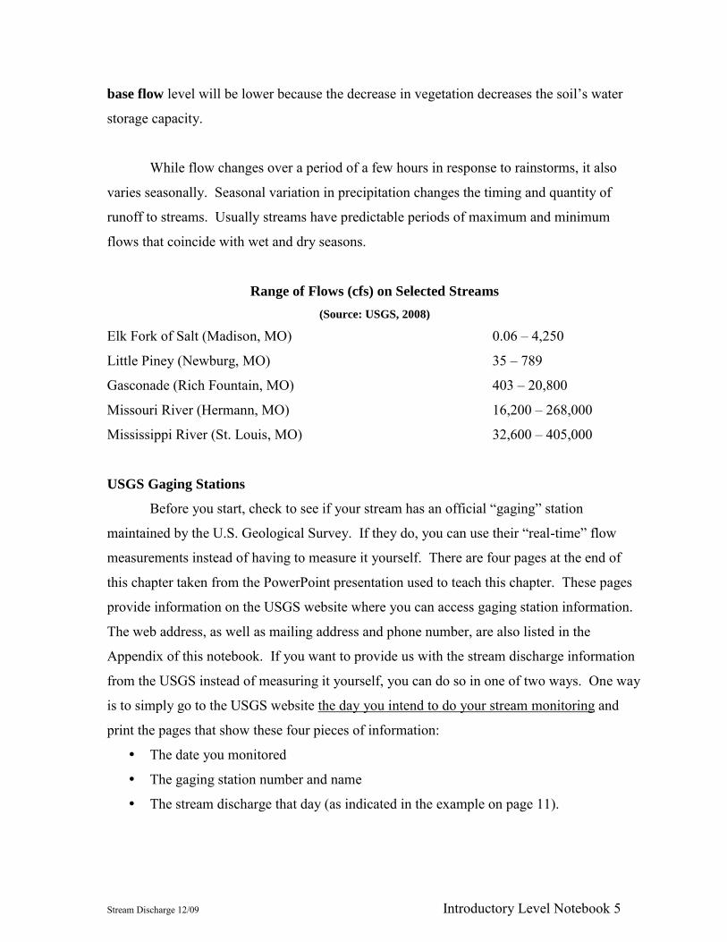
While flow changes over a period of a few hours in response to rainstorms, it also

varies seasonally. Seasonal variation in precipitation changes the timing and quantity of

runoff to streams. Usually streams have predictable periods of maximum and minimum

flows that coincide with wet and dry seasons.

Range of Flows (cfs) on Selected Streams

(Source: USGS, 2008)

Elk Fork of Salt (Madison, MO) 0.06 – 4,250

Little Piney (Newburg, MO) 35 – 789

Gasconade (Rich Fountain, MO) 403 – 20,800

Missouri River (Hermann, MO) 16,200 – 268,000

Mississippi River (St. Louis, MO) 32,600 – 405,000

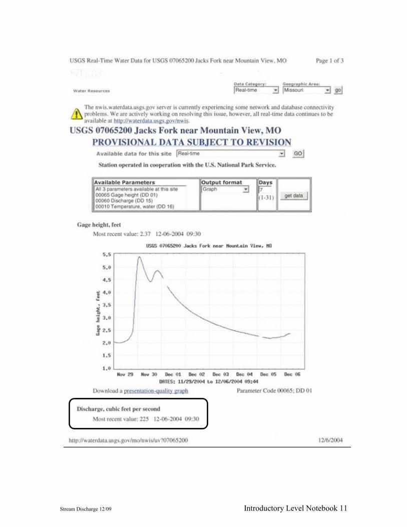
USGS Gaging Stations

Before you start, check to see if your stream has an official “gaging” station

maintained by the U.S. Geological Survey. If they do, you can use their “real-time” flow

measurements instead of having to measure it yourself. There are four pages at the end of

this chapter taken from the PowerPoint presentation used to teach this chapter. These pages

provide information on the USGS website where you can access gaging station information.

The web address, as well as mailing address and phone number, are also listed in the

Appendix of this notebook. If you want to provide us with the stream discharge information

from the USGS instead of measuring it yourself, you can do so in one of two ways. One way

is to simply go to the USGS website the day you intend to do your stream monitoring and

print the pages that show these four pieces of information:

The date you monitored

The gaging station number and name

The stream discharge that day (as indicated in the example on page 11).


On the computer screen it will look like one long page, but when you print the page,

it will probably be at least two pages. You can submit the pages along with your Site

Selection and/or Macroinvertebrate Data Sheets.

Or, if you don’t want to print and send the pages, you can write this information

under “Comments” on the Macroinvertebrate Data Sheet:

Date

Number and name of the gaging station (e.g., “USGS 07065200 Jacks Fork near

Mountain View, MO”)

The stream discharge in cubic feet per second (e.g., “225 ft3/sec”).

How to Measure Discharge

If you are not lucky enough to have a gaging station nearby, here’s one way to

measure flow yourself. Select a stream section that is relatively straight, free of large objects

such as logs or boulders, with a noticeable current and with a depth as uniform as possible.

See Data Sheet on page 9-10 for an example.

1. Determine the stream cross sectional area

Stretch a tape measure marked in tenths of a foot (not inches) across the stream

(provided by program). The “0” point should be anchored at the wetted edge of the

stream. The opposite end of the tape measure should be anchored so that it is taut and

perpendicular to the flow. Measure the width of the stream from wetted perimeter to

wetted perimeter in tenths of a foot and record the width on the Stream Discharge

Worksheet.

With the tape measure still attached to the stream banks, measure the stream depth at

intervals across the stream. Record this information on the first page of your Stream

Discharge Worksheet. For streams less than 20 feet wide, measure the depth

every foot. For streams greater than 20 feet wide, measure the depth every two

feet. Remember that the depth must be measured in feet and tenths of a foot

(e.g., 0.5 ft., 1.2 ft.) and NOT in inches (e.g., 6 inches, or, 1 ft. 2 inches).


2. Determining the Average Surface Velocity for the stream

Pick several points at intervals across the stream approximately equal distance apart

for velocity measurements. For streams less than ten feet wide, take three

measurements. For streams greater than ten feet wide, conduct no fewer than

four velocity measurements. Once you have determined the number of velocity

float trials you need, measure the water’s surface velocity in the following manner:

Select two points approximately equal distance upstream and downstream from the

tape measure you have stretched across the stream; five feet above and five feet

below the tape measure works well for most Missouri streams. However, this will be

dependent on the swiftness of the stream. In faster water, you may want this distance

to be greater, while in slow waters, you may wish this distance to be shorter.

Determine the distance between these two points and record this value (in feet) on the

Stream Discharge Worksheet.

Drop a mutually-buoyant practice (wiffle) golf ball (provided by program) above the

upstream point and record the time it takes to float to the downstream point (in

seconds). Record each float time on the Stream Discharge Worksheet.

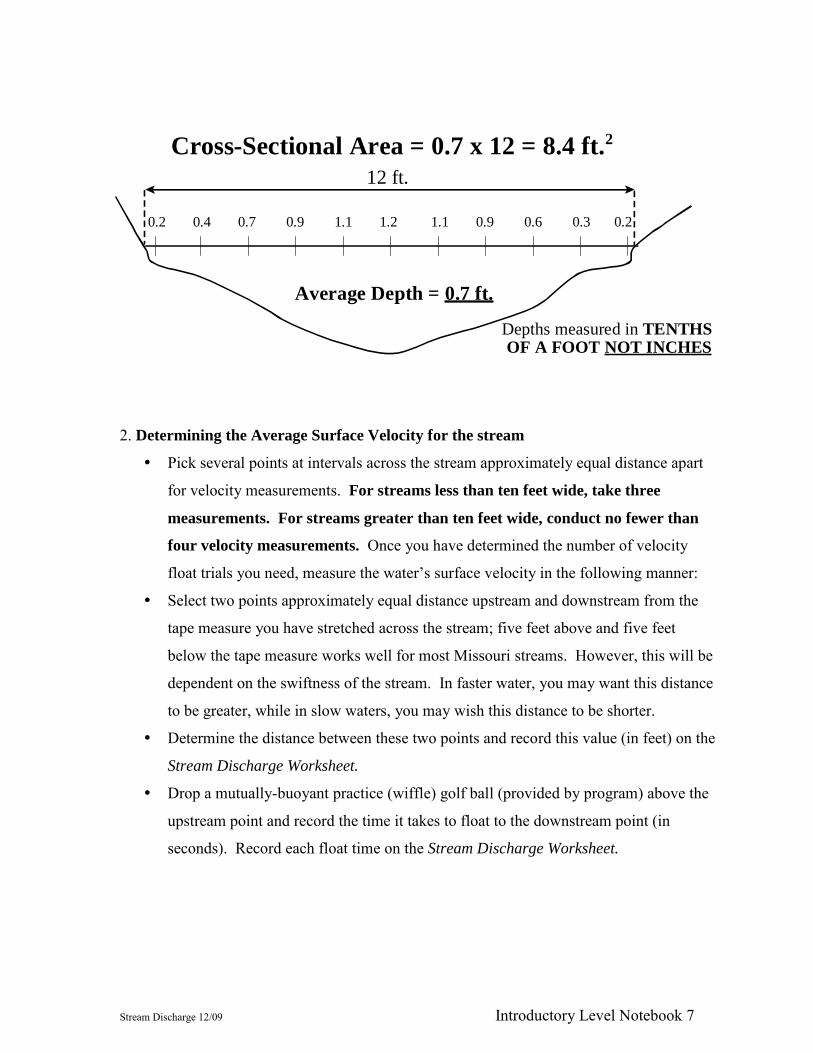
Depths measured in TENTHS OF A FOOT NOT INCHES

0.2 0.4 0.7 0.9 1.1 1.2 0.91.1 0.6 0.3 0.2

12 ft.

Cross-Sectional Area = 0.7 x 12 = 8.4 ft.2

Average Depth = 0.7 ft.


This technique will be demonstrated in the field during the training class. Also,

complete instructions are printed on the Stream Discharge Worksheet itself, which serves as

a handy reference when you are out sampling. As an example, we’ve included a completed

form at the end of this chapter.

Materials Needed to Measure Stream Discharge

1. 100-foot tape measure, marked in tenths of a foot (provided by program)

2. A mutually-buoyant float - for example, a practice, wiffle golf ball (provided by program)

3. Two sticks or metal pins (provided by volunteer)

4. Stick with depths marked in tenths of a foot (provided by volunteer)

5. Stopwatch or watch with a second hand (provided by volunteer)

6. 10-foot-long rope (provided by volunteer)

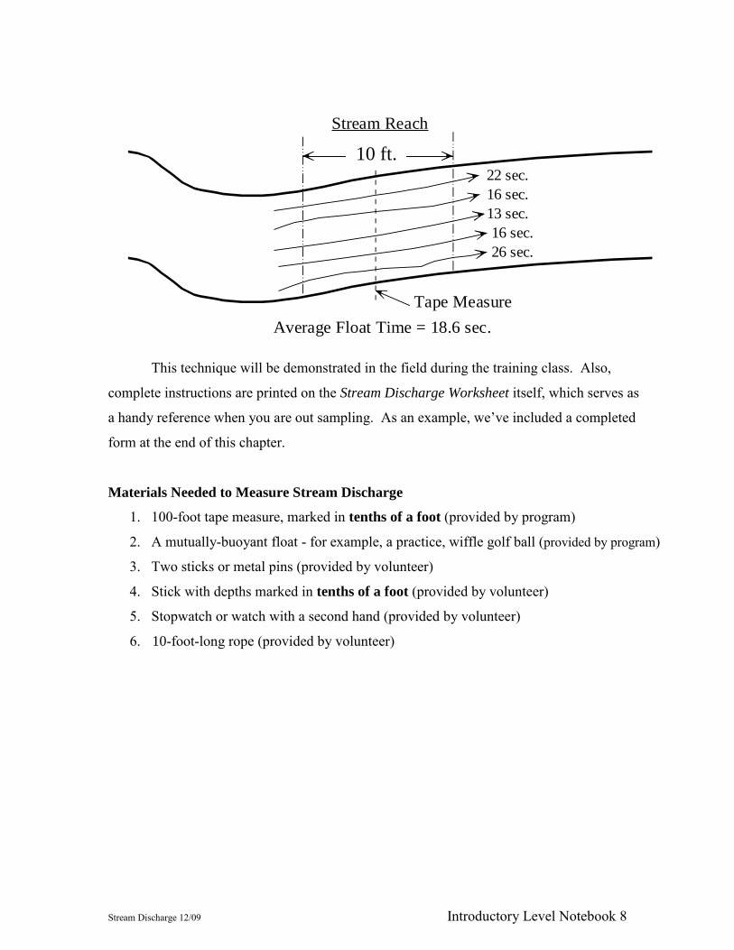
Stream Reach

10 ft.

Tape Measure

22 sec.

16 sec.

13 sec.

16 sec.

26 sec.

Average Float Time = 18.6 sec.

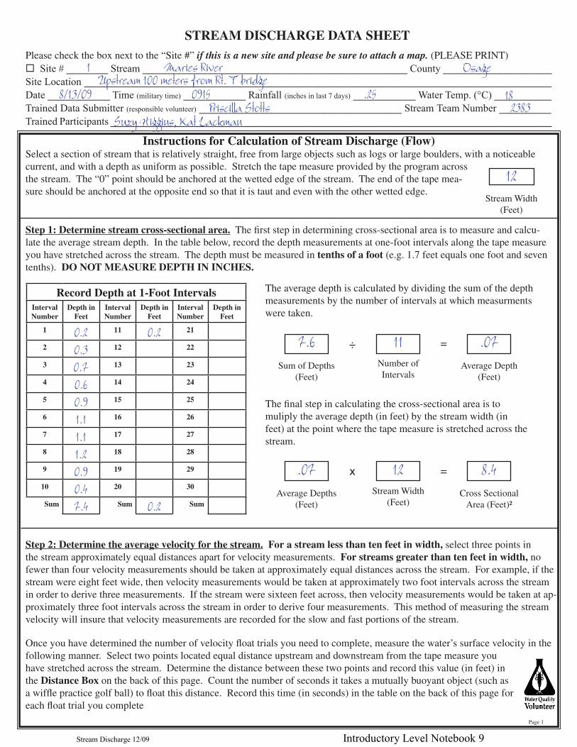
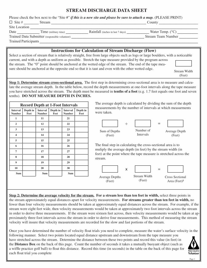
STREAM DISCHARGE DATA SHEETPlease check the box next to the “Site #” if this is a new site and please be sure to attach a map. (PLEASE PRINT) Site # ________ Stream ___________________________________________________ County _____________________Site Location __________________________________________________________________________________________Date ____________ Time (military time) ____________ Rainfall (inches in last 7 days) ____________ Water Temp. (°C) ___________Trained Data Submitter (responsible volunteer) _______________________________________ Stream Team Number __________Trained Participants _____________________________________________________________________________________

Instructions for Calculation of Stream Discharge (Flow)Select a section of stream that is relatively straight, free from large objects such as logs or large boulders, with a noticeable current, and with a depth as uniform as possible. Stretch the tape measure provided by the program across the stream. The “0” point should be anchored at the wetted edge of the stream. The end of the tape mea-sure should be anchored at the opposite end so that it is taut and even with the other wetted edge.

Step 1: Determine stream cross-sectional area. The first step in determining cross-sectional area is to measure and calcu-late the average stream depth. In the table below, record the depth measurements at one-foot intervals along the tape measure you have stretched across the stream. The depth must be measured in tenths of a foot (e.g. 1.7 feet equals one foot and seven tenths). DO NOT MEASURE DEPTH IN INCHES.

Step 2: Determine the average velocity for the stream. For a stream less than ten feet in width, select three points in the stream approximately equal distances apart for velocity measurements. For streams greater than ten feet in width, no fewer than four velocity measurements should be taken at approximately equal distances across the stream. For example, if the stream were eight feet wide, then velocity measurements would be taken at approximately two foot intervals across the stream in order to derive three measurements. If the stream were sixteen feet across, then velocity measurements would be taken at ap-proximately three foot intervals across the stream in order to derive four measurements. This method of measuring the stream velocity will insure that velocity measurements are recorded for the slow and fast portions of the stream.

Once you have determined the number of velocity float trials you need to complete, measure the water’s surface velocity in the following manner. Select two points located equal distance upstream and downstream from the tape measure you have stretched across the stream. Determine the distance between these two points and record this value (in feet) in the Distance Box on the back of this page. Count the number of seconds it takes a mutually buoyant object (such as a wiffle practice golf ball) to float this distance. Record this time (in seconds) in the table on the back of this page for each float trial you complete

Record Depth at 1-Foot IntervalsInterval Number

Depth in Feet

Interval Number

Depth in Feet

Interval Number

Depth in Feet

1 0.2 11 0.2 21

2 0.3 12 22

3 0.7 13 23

4 0.6 14 24

5 0.9 15 25

6 1.1 16 26

7 1.1 17 27

8 1.2 18 28

9 0.9 19 29

10 0.4 20 30

Sum 7.4 Sum 0.2 Sum

Page 1

Stream Width(Feet)

12

The average depth is calculated by dividing the sum of the depth measurements by the number of intervals at which measurments were taken.

Sum of Depths(Feet)

7.6Number of Intervals

11Average Depth

(Feet)

.07÷ =

The final step in calculating the cross-sectional area is to muliply the average depth (in feet) by the stream width (in feet) at the point where the tape measure is stretched across the stream.

Average Depths(Feet)

.07Stream Width

(Feet)

12Cross Sectional

Area (Feet)²

8.4x =

1 Maries River OsageUpstream 100 meters from Rt. T bridge

8/13/09 0915Priscilla Stotts

18.252383

Suzy Higgins, Kat Lackman


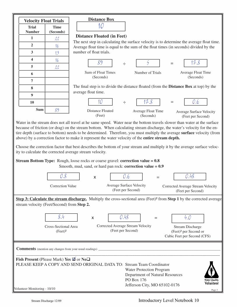
Water in the stream does not all travel at he same speed. Water near the bottom travels slower than water at the surface because of friction (or drag) on the stream bottom. When calculating stream discharge, the water’s velocity for the en-tire depth (surface to bottom) needs to be determined. Therefore, you must multiply the average surface velocity (from above) by a correction factor to make it represent the water velocity of the entire stream depth.

Choose the correction factor that best describes the bottom of your stream and multiply it by the average surface veloc-ity to calculate the corrected average stream velocity.

Stream Bottom Type: Rough, loose rocks or coarse gravel: correction value = 0.8 Smooth, mud, sand, or hard pan rock: correction value = 0.9

Step 3: Calculate the stream discharge. Multiply the cross-sectional area (Feet)² from Step 1 by the corrected average stream velocity (Feet/Second) from Step 2.

Comments (mention any changes from your usual readings) ________________________________________________________________________________________________________________________________________________________________________

Fish Present (Please Mark) Yes or NoPLEASE KEEP A COPY AND SEND ORIGINAL DATA TO: Stream Team Coordinator

Water Protection ProgramDepartment of Natural ResourcesPO Box 176Jefferson City, MO 65102-0176

Page 2

Velocity Float TrialsTrial

NumberTime

(Seconds)

1 222 163 134 165 226

7

8

9

10

Sum 89

Distance Box

Distance Floated (in Feet)

10

Correction Value

0.8Average Surface Velocity

(Feet per Second)

0.6Corrected Average Stream Velocity

(Feet per Second)

0.48x =

Cross-Sectional Area(Feet)²

8.4Corrected Average Stream Velocity

(Feet per Second)

0.48Stream Discharge

(Feet)³ per Second orCubic Feet per Second (CFS)

4.0x =

The next step in calculating the surface velocity is to determine the average float time. Average float time is equal to the sum of the float times (in seconds) divided by the number of float trials.

Sum of Float Times(Seconds)

89Number of Trials

5Average Float Time

(Seconds)

17.8÷ =

The final step is to divide the distance floated (from the Distance Box at top) by the average float time.

Distance Floated(Feet)

10Average Float Time

(Seconds)

17.8Average Surface Velocity

(Feet per Second)

0.6÷ =

Volunteer Monitoring - 10/10


Instructions for Calculation of Stream Discharge (Flow)Select a section of stream that is relatively straight, free from large objects such as logs or large boulders, with a noticeable current, and with a depth as uniform as possible. Stretch the tape measure provided by the program across the stream. The “0” point should be anchored at the wetted edge of the stream. The end of the tape mea-sure should be anchored at the opposite end so that it is taut and even with the other wetted edge.

Step 1: Determine stream cross-sectional area. The first step in determining cross-sectional area is to measure and calcu-late the average stream depth. In the table below, record the depth measurements at one-foot intervals along the tape measure you have stretched across the stream. The depth must be measured in tenths of a foot (e.g. 1.7 feet equals one foot and seven tenths). DO NOT MEASURE DEPTH IN INCHES.

Step 2: Determine the average velocity for the stream. For a stream less than ten feet in width, select three points in the stream approximately equal distances apart for velocity measurements. For streams greater than ten feet in width, no fewer than four velocity measurements should be taken at approximately equal distances across the stream. For example, if the stream were eight feet wide, then velocity measurements would be taken at approximately two foot intervals across the stream in order to derive three measurements. If the stream were sixteen feet across, then velocity measurements would be taken at ap-proximately three foot intervals across the stream in order to derive four measurements. This method of measuring the stream velocity will insure that velocity measurements are recorded for the slow and fast portions of the stream.

Once you have determined the number of velocity float trials you need to complete, measure the water’s surface velocity in the following manner. Select two points located equal distance upstream and downstream from the tape measure you have stretched across the stream. Determine the distance between these two points and record this value (in feet) in the Distance Box on the back of this page. Count the number of seconds it takes a mutually buoyant object (such as a wiffle practice golf ball) to float this distance. Record this time (in seconds) in the table on the back of this page for each float trial you complete

STREAM DISCHARGE DATA SHEETPlease check the box next to the “Site #” if this is a new site and please be sure to attach a map. (PLEASE PRINT) Site # ________ Stream ___________________________________________________ County _____________________Site Location __________________________________________________________________________________________Date ____________ Time (military time) ____________ Rainfall (inches in last 7 days) ____________ Water Temp. (°C) ___________Trained Data Submitter (responsible volunteer) _______________________________________ Stream Team Number __________Trained Participants _____________________________________________________________________________________

Record Depth at 1-Foot IntervalsInterval Number

Depth in Feet

Interval Number

Depth in Feet

Interval Number

Depth in Feet

1 11 21

2 12 22

3 13 23

4 14 24

5 15 25

6 16 26

7 17 27

8 18 28

9 19 29

10 20 30

Sum Sum Sum

Page 1

Stream Width(Feet)

The average depth is calculated by dividing the sum of the depth measurements by the number of intervals at which measurments were taken.

Sum of Depths(Feet)

Number of Intervals

Average Depth(Feet)

÷ =

The final step in calculating the cross-sectional area is to muliply the average depth (in feet) by the stream width (in feet) at the point where the tape measure is stretched across the stream.

Average Depths(Feet)

Stream Width(Feet)

Cross SectionalArea (Feet)²

x =

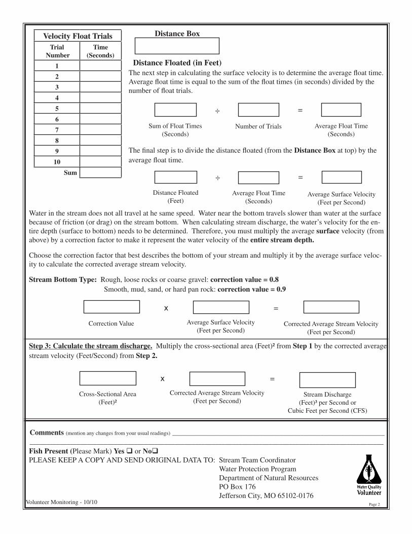
Water in the stream does not all travel at he same speed. Water near the bottom travels slower than water at the surface because of friction (or drag) on the stream bottom. When calculating stream discharge, the water’s velocity for the en-tire depth (surface to bottom) needs to be determined. Therefore, you must multiply the average surface velocity (from above) by a correction factor to make it represent the water velocity of the entire stream depth.

Choose the correction factor that best describes the bottom of your stream and multiply it by the average surface veloc-ity to calculate the corrected average stream velocity.

Stream Bottom Type: Rough, loose rocks or coarse gravel: correction value = 0.8 Smooth, mud, sand, or hard pan rock: correction value = 0.9

Step 3: Calculate the stream discharge. Multiply the cross-sectional area (Feet)² from Step 1 by the corrected average stream velocity (Feet/Second) from Step 2.

Comments (mention any changes from your usual readings) ________________________________________________________________________________________________________________________________________________________________________

Fish Present (Please Mark) Yes or NoPLEASE KEEP A COPY AND SEND ORIGINAL DATA TO: Stream Team Coordinator

Water Protection ProgramDepartment of Natural ResourcesPO Box 176Jefferson City, MO 65102-0176

Page 2

Velocity Float TrialsTrial

NumberTime

(Seconds)

1

2

3

4

5

6

7

8

9

10

Sum

Distance Box

Distance Floated (in Feet)

Correction Value Average Surface Velocity (Feet per Second)

Corrected Average Stream Velocity(Feet per Second)

x =

Cross-Sectional Area(Feet)²

Corrected Average Stream Velocity(Feet per Second)

Stream Discharge(Feet)³ per Second or

Cubic Feet per Second (CFS)

x =

The next step in calculating the surface velocity is to determine the average float time. Average float time is equal to the sum of the float times (in seconds) divided by the number of float trials.

Sum of Float Times(Seconds)

Number of Trials Average Float Time(Seconds)

÷ =

The final step is to divide the distance floated (from the Distance Box at top) by the average float time.

Distance Floated(Feet)

Average Float Time(Seconds)

Average Surface Velocity(Feet per Second)

÷ =

Volunteer Monitoring - 10/10

Chapter 3 Stream Discharge - Missouri … Discharge 12/09 Introductory Level Notebook 1 Chapter 3...

Documents

Transcript of Chapter 3 Stream Discharge - Missouri … Discharge 12/09 Introductory Level Notebook 1 Chapter 3...