Chapter 3 Solving problems by searching - Bilkent...
118
CS461 Artificial Intelligence © Pinar Duygulu Spring 2008 1 Chapter 3 Solving problems by searching CS 461 – Artificial Intelligence Pinar Duygulu Bilkent University, Spring 2008 Slides are mostly adapted from AIMA and MIT Open Courseware
Transcript of Chapter 3 Solving problems by searching - Bilkent...
CS461 Artificial Intelligence © Pinar Duygulu Spring 2008
1
Chapter 3Solving problems by searching
CS 461 – Artificial IntelligencePinar Duygulu
Bilkent University, Spring 2008
Slides are mostly adapted from AIMA and MIT Open Courseware
CS461 Artificial Intelligence © Pinar Duygulu Spring 2008
2
Introduction
• Simple-reflex agents directly maps states to actions. • Therefore, they cannot operate well in environments
where the mapping is too large to store or takes too much to learn
• Goal-based agents can succeed by considering future actions and desirability of their outcomes
• Problem solving agent is a goal-based agent that decides what to do by finding sequences of actions that lead to desirable states
CS461 Artificial Intelligence © Pinar Duygulu Spring 2008
3
Outline
• Problem-solving agents• Problem types• Problem formulation• Example problems• Basic search algorithms
CS461 Artificial Intelligence © Pinar Duygulu Spring 2008
4
Problem solving agents
• Intelligent agents are supposed to maximize their performance measure
• This can be simplified if the agent can adopt a goal and aim at satisfying it
• Goals help organize behaviour by limiting the objectives that the agent is trying to achieve
• Goal formulation, based on the current situation and the agent’s performance measure, is the first step in problem solving
• Goal is a set of states. The agent’s task is to find out which sequence of actions will get it to a goal state
• Problem formulation is the process of deciding what sorts of actions and states to consider, given a goal
CS461 Artificial Intelligence © Pinar Duygulu Spring 2008
5
Problem solving agents
• An agent with several immediate options of unknown value can decide what to do by first examining different possible sequences of actions that lead to states of known value, and then choosing the best sequence
• Looking for such a sequence is called search• A search algorithm takes a problem as input and returns a
solution in the form of action sequence• One a solution is found the actions it recommends can be
carried out – execution phase
CS461 Artificial Intelligence © Pinar Duygulu Spring 2008
6
Problem solving agents
• “formulate, search, execute” design for the agent• After formulating a goal and a problem to solve the agent
calls a search procedure to solve it• It then uses the solution to guide its actions, doing whatever
the solution recommends as the next thing to do (typically the first action in the sequence)
• Then removing that step from the sequence• Once the solution has been executed, the agent will
formulate a new goal
CS461 Artificial Intelligence © Pinar Duygulu Spring 2008
7
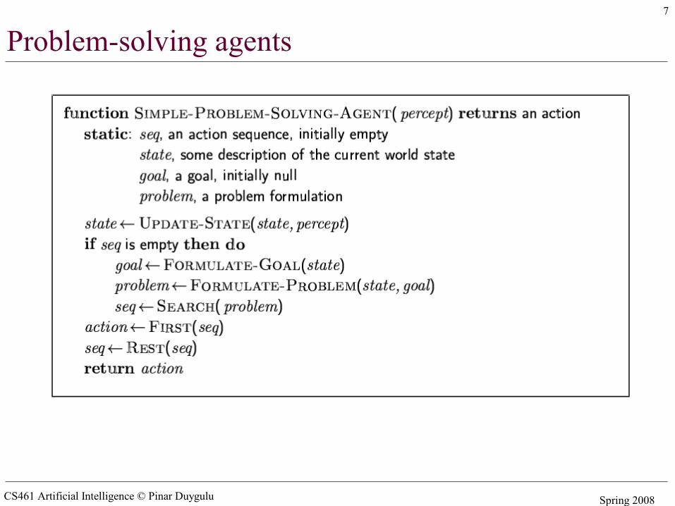
Problem-solving agents
CS461 Artificial Intelligence © Pinar Duygulu Spring 2008
8
Environment Assumptions
• Static, formulating and solving the problem is done without paying attention to any changes that might be occurring in the environment
• Initial state is known and the environment is observable
• Discrete, enumerate alternative courses of actions• Deterministic, solutions to problems are single
sequences of actions, so they cannot handle any unexpected events, and solutions are executed without paying attention to the percepts
CS461 Artificial Intelligence © Pinar Duygulu Spring 2008
9
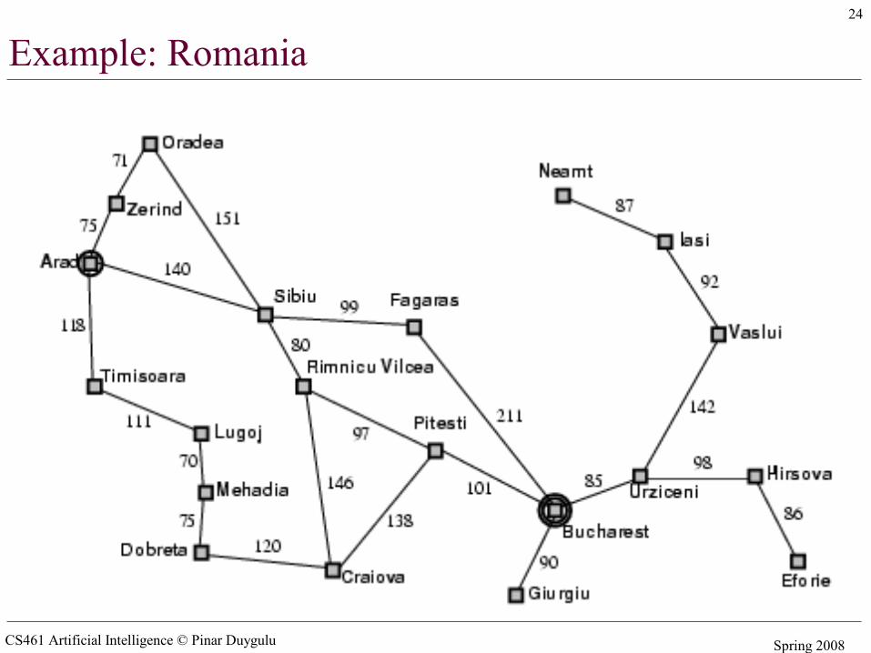
Example: Romania
• On holiday in Romania; currently in Arad.• Flight leaves tomorrow from Bucharest• Formulate goal:
– be in Bucharest• Formulate problem:
– states: various cities– actions: drive between cities
• Find solution:– sequence of cities, e.g., Arad, Sibiu, Fagaras, Bucharest

CS461 Artificial Intelligence © Pinar Duygulu Spring 2008
10
Example: Romania
CS461 Artificial Intelligence © Pinar Duygulu Spring 2008
11
Well-defined problems and solutions• A problem can be defined formally by four components• Initial state that the agent starts in
– e.g. In(Arad)• A description of the possible actions available to the agent
– Successor function – returns a set of <action,successor> pairs– e.g. {<Go(Sibiu),In(Sibiu)>, <Go(Timisoara),In(Timisoara)>, <Go(Zerind), In(Zerind)>}
– Initial state and the successor function define the state space ( a graph in which the nodes are states and the arcs between nodes are actions). A path in state space is a sequence of states connected by a sequence of actions
• Goal test determines whether a given state is a goal state– e.g.{In(Bucharest)}
• Path cost function that assigns a numeric cost to each path. The cost of a path can be described as the some of the costs of the individual actions along the path – step cost– e.g. Time to go Bucharest
CS461 Artificial Intelligence © Pinar Duygulu Spring 2008
12
Problem Formulation• A solution to a problem is a path from the initial state to the
goal state• Solution quality is measured by the path cost function and an
optimal solution has the lowest path cost among all solutions• Real world is absurdly complex
– state space must be abstracted for problem solving• (Abstract) state = set of real states• (Abstract) action = complex combination of real actions
– e.g., "Arad Zerind" represents a complex set of possible routes, detours, rest stops, etc.
• For guaranteed realizability, any real state "in Arad“ must get to some real state "in Zerind"
• (Abstract) solution = – set of real paths that are solutions in the real world
• Each abstract action should be "easier" than the original problem
CS461 Artificial Intelligence © Pinar Duygulu Spring 2008
13
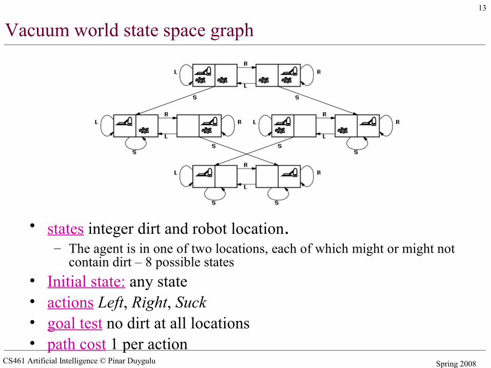
Vacuum world state space graph
• states integer dirt and robot location.– The agent is in one of two locations, each of which might or might not
contain dirt – 8 possible states• Initial state: any state• actions Left, Right, Suck• goal test no dirt at all locations• path cost 1 per action
CS461 Artificial Intelligence © Pinar Duygulu Spring 2008
14
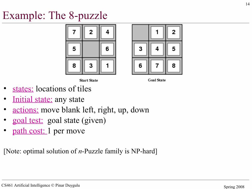
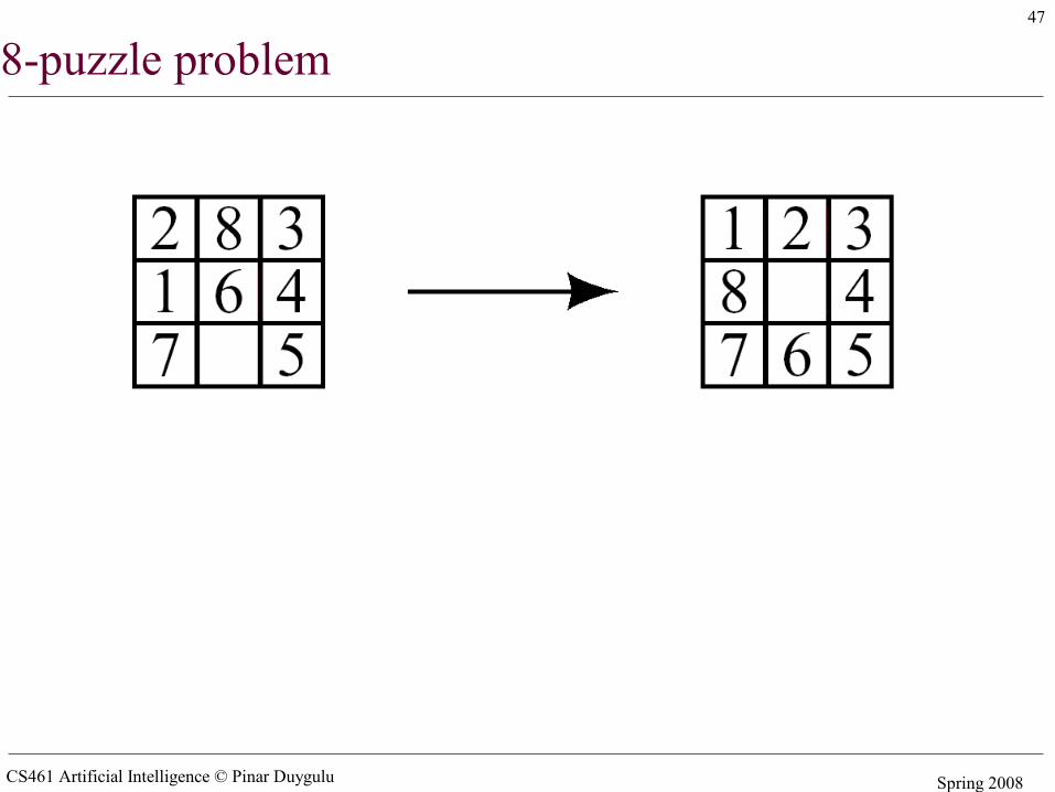
Example: The 8-puzzle
• states: locations of tiles • Initial state: any state• actions: move blank left, right, up, down • goal test: goal state (given)• path cost: 1 per move
[Note: optimal solution of n-Puzzle family is NP-hard]
CS461 Artificial Intelligence © Pinar Duygulu Spring 2008
15
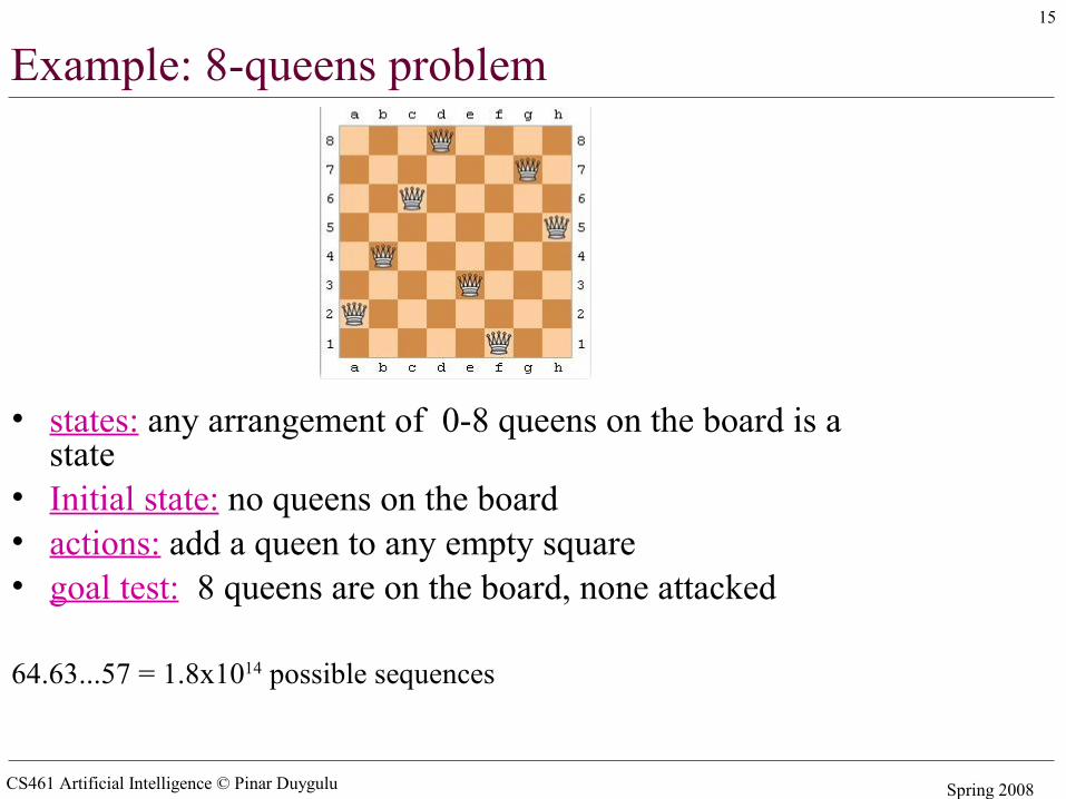
Example: 8-queens problem
• states: any arrangement of 0-8 queens on the board is a state
• Initial state: no queens on the board• actions: add a queen to any empty square • goal test: 8 queens are on the board, none attacked
64.63...57 = 1.8x10¹⁴ possible sequences
CS461 Artificial Intelligence © Pinar Duygulu Spring 2008
16
Example: Route finding problem
• states: each is represented by a location (e.g. An airport) and the current time
• Initial state: specified by the problem• Successor function: returns the states resulting from taking any
scheduled flight, leaving later than the current time plus the within airport transit time, from the current airport to another
• goal test: are we at the destination by some pre-specified time• Path cost:monetary cost, waiting time, flight time, customs and
immigration procedures, seat quality, time of day, type of airplane, frequent-flyer mileage awards, etc
• Route finding algorithms are used in a variety of applications, such as routing in computer networks, military operations planning, airline travel planning systems
CS461 Artificial Intelligence © Pinar Duygulu Spring 2008
17
Other example problems
• Touring problems: visit every city at least once, starting and ending at Bucharest
• Travelling salesperson problem (TSP) : each city must be visited exactly once – find the shortest tour
• VLSI layout design: positioning millions of components and connections on a chip to minimize area, minimize circuit delays, minimize stray capacitances, and maximize manufacturing yield
• Robot navigation• Internet searching• Automatic assembly sequencing• Protein design
CS461 Artificial Intelligence © Pinar Duygulu Spring 2008
18
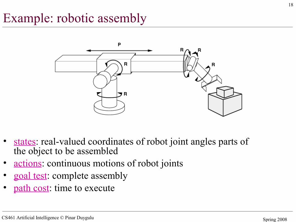
Example: robotic assembly
• states: real-valued coordinates of robot joint angles parts of the object to be assembled
• actions: continuous motions of robot joints• goal test: complete assembly• path cost: time to execute
CS461 Artificial Intelligence © Pinar Duygulu Spring 2008
19
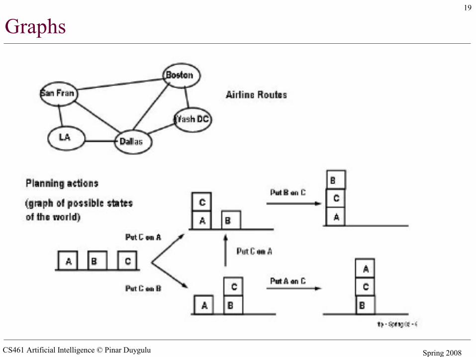
Graphs
CS461 Artificial Intelligence © Pinar Duygulu Spring 2008
20
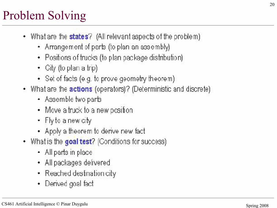
Problem Solving
CS461 Artificial Intelligence © Pinar Duygulu Spring 2008
21
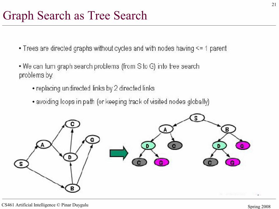
Graph Search as Tree Search
CS461 Artificial Intelligence © Pinar Duygulu Spring 2008
22
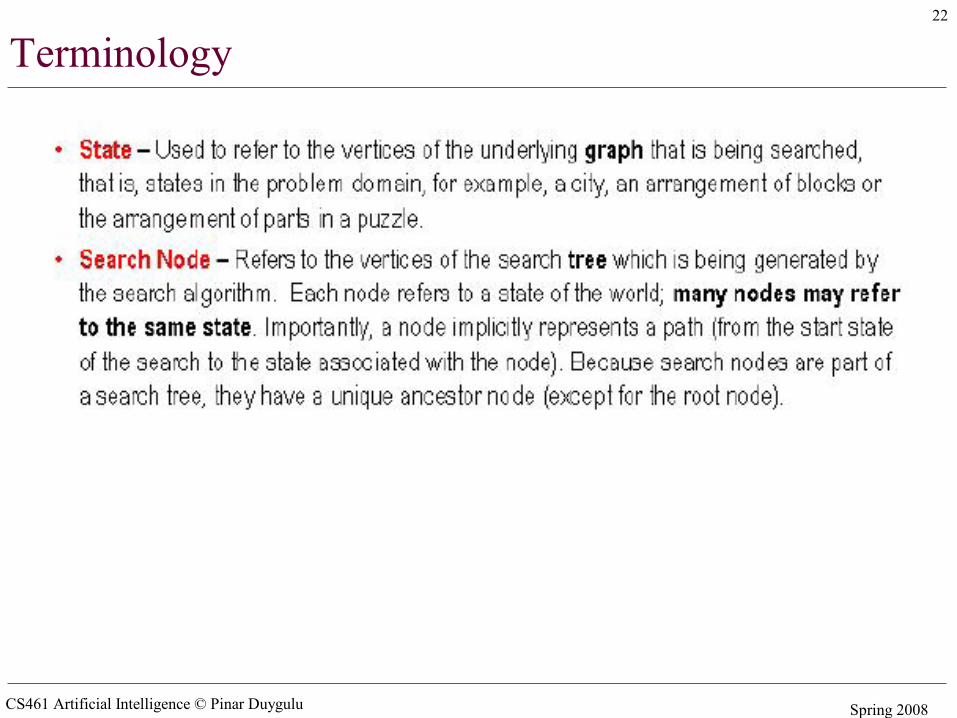
Terminology
CS461 Artificial Intelligence © Pinar Duygulu Spring 2008
23
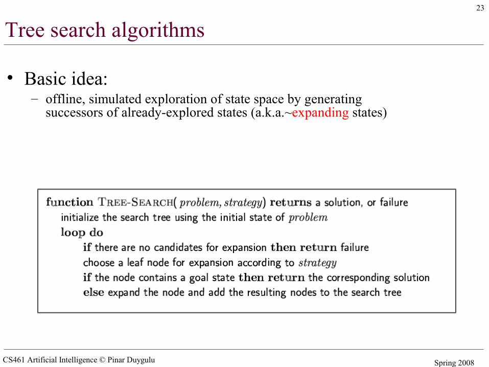
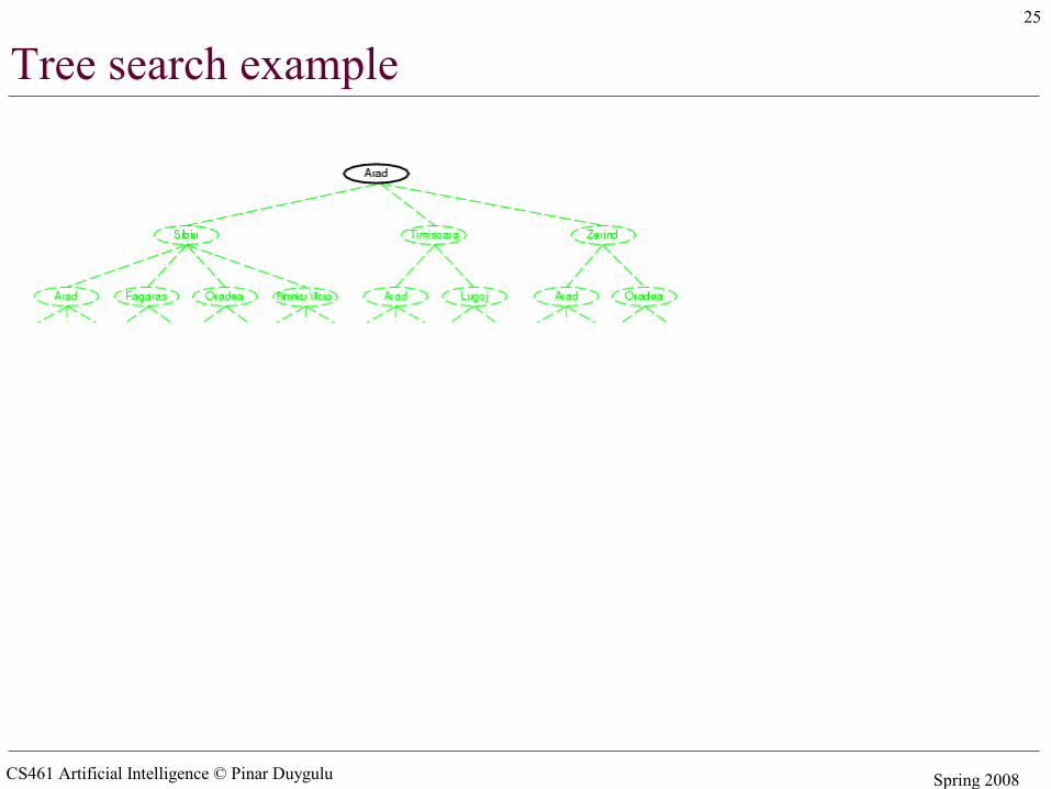
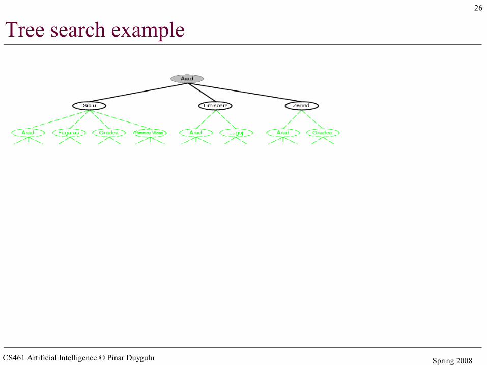
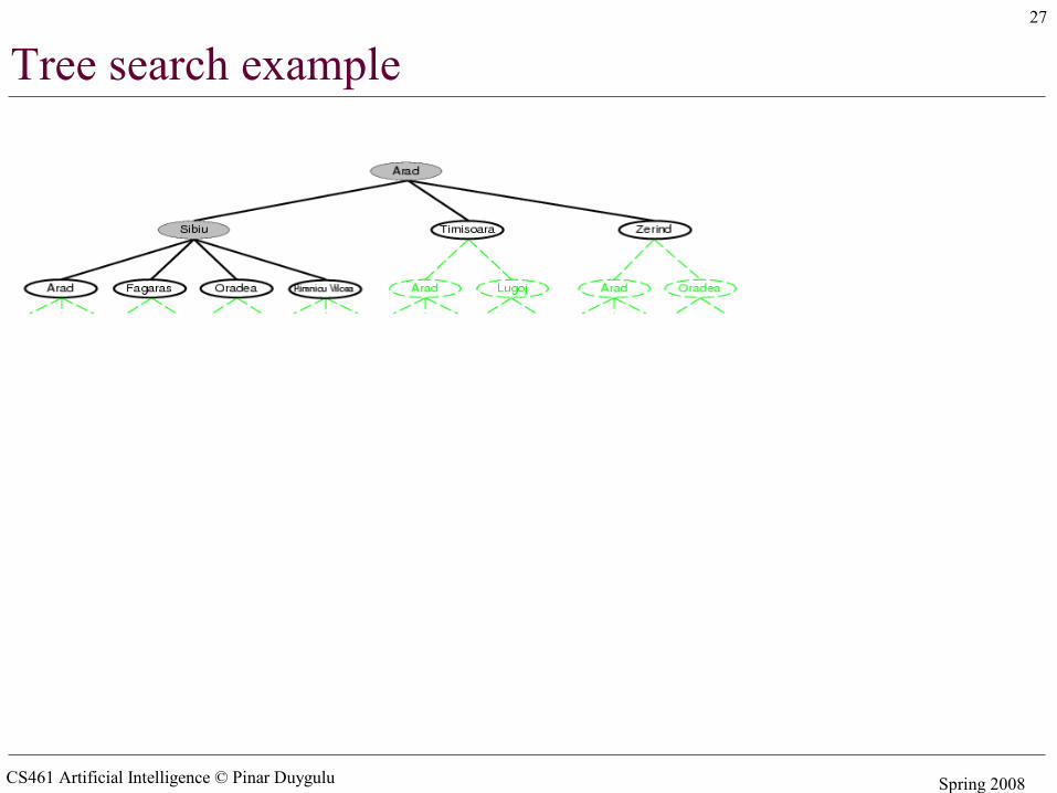
Tree search algorithms
• Basic idea:– offline, simulated exploration of state space by generating
successors of already-explored states (a.k.a.~expanding states)
CS461 Artificial Intelligence © Pinar Duygulu Spring 2008
24
Example: Romania
CS461 Artificial Intelligence © Pinar Duygulu Spring 2008
25
Tree search example
CS461 Artificial Intelligence © Pinar Duygulu Spring 2008
26
Tree search example
CS461 Artificial Intelligence © Pinar Duygulu Spring 2008
27
Tree search example
CS461 Artificial Intelligence © Pinar Duygulu Spring 2008
28
Implementation: Components of a node
• State: the state in the state space to which the node corresponds
• Parent-node: the node in the search tree that generated this node
• Action: the action that was applied to the parent to generate the node
• Path-cost: the cost, traditionally denoted by g(n), of the path from the initial state to the node, as indicated by the parent pointers
• Depth: the number of steps along the path from the initial state
CS461 Artificial Intelligence © Pinar Duygulu Spring 2008
29
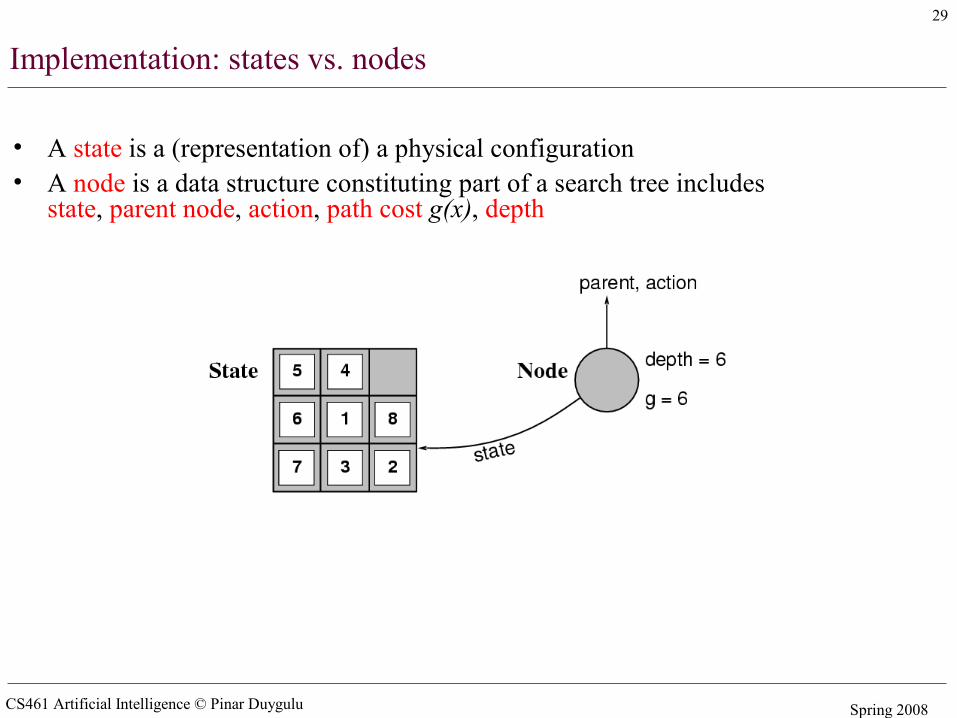
Implementation: states vs. nodes
• A state is a (representation of) a physical configuration• A node is a data structure constituting part of a search tree includes
state, parent node, action, path cost g(x), depth
CS461 Artificial Intelligence © Pinar Duygulu Spring 2008
30
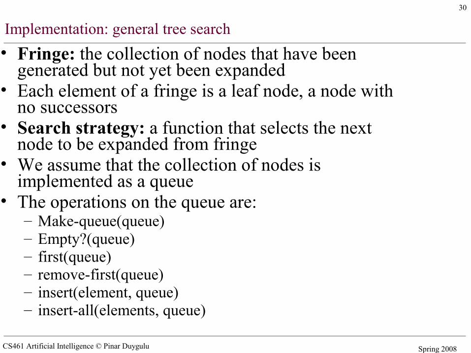
Implementation: general tree search• Fringe: the collection of nodes that have been
generated but not yet been expanded• Each element of a fringe is a leaf node, a node with
no successors• Search strategy: a function that selects the next
node to be expanded from fringe• We assume that the collection of nodes is
implemented as a queue• The operations on the queue are:
– Make-queue(queue)– Empty?(queue)– first(queue)– remove-first(queue)– insert(element, queue)– insert-all(elements, queue)
CS461 Artificial Intelligence © Pinar Duygulu Spring 2008
31
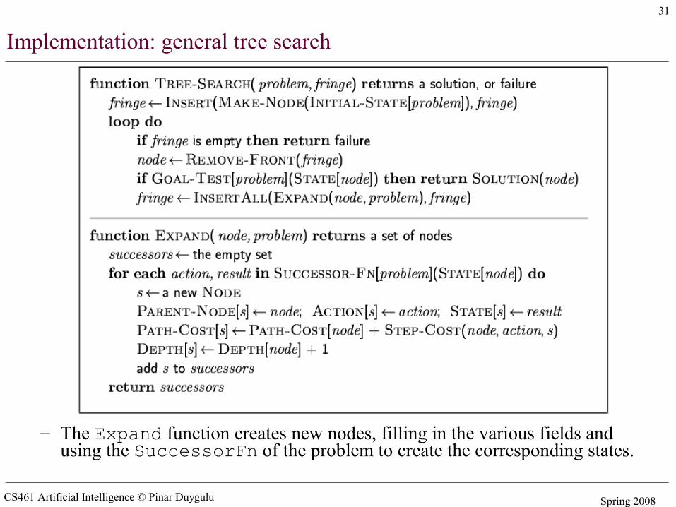
Implementation: general tree search
– The Expand function creates new nodes, filling in the various fields and using the SuccessorFn of the problem to create the corresponding states.
CS461 Artificial Intelligence © Pinar Duygulu Spring 2008
32
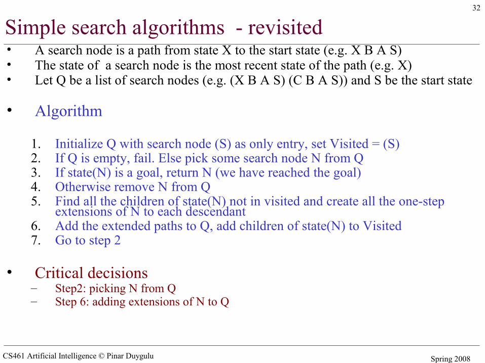
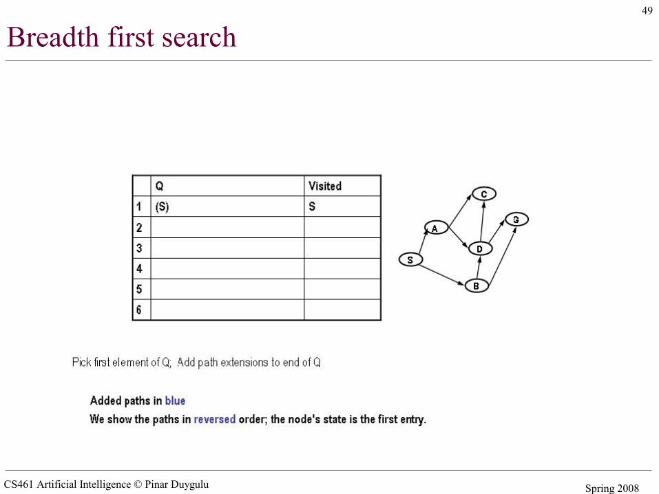
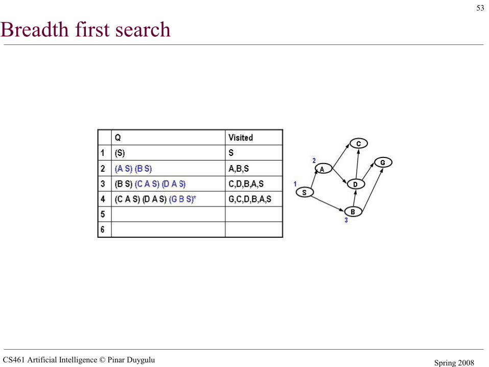
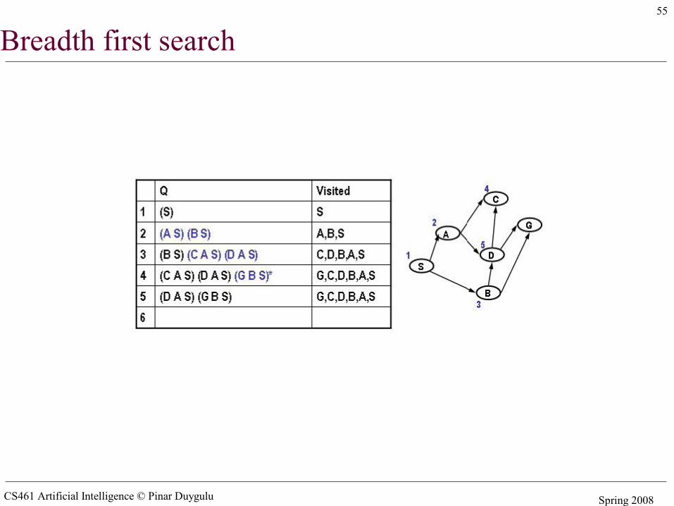
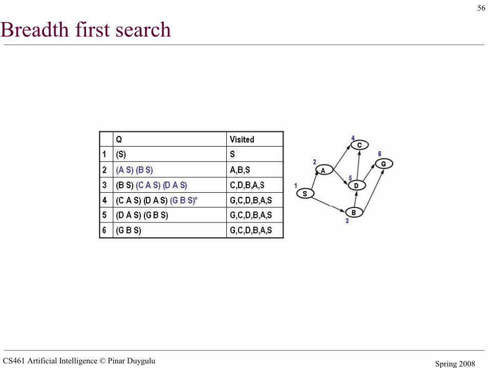
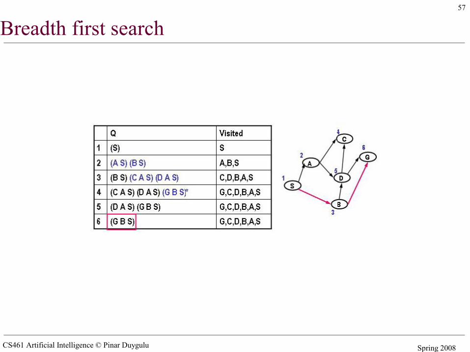
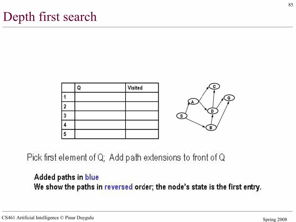
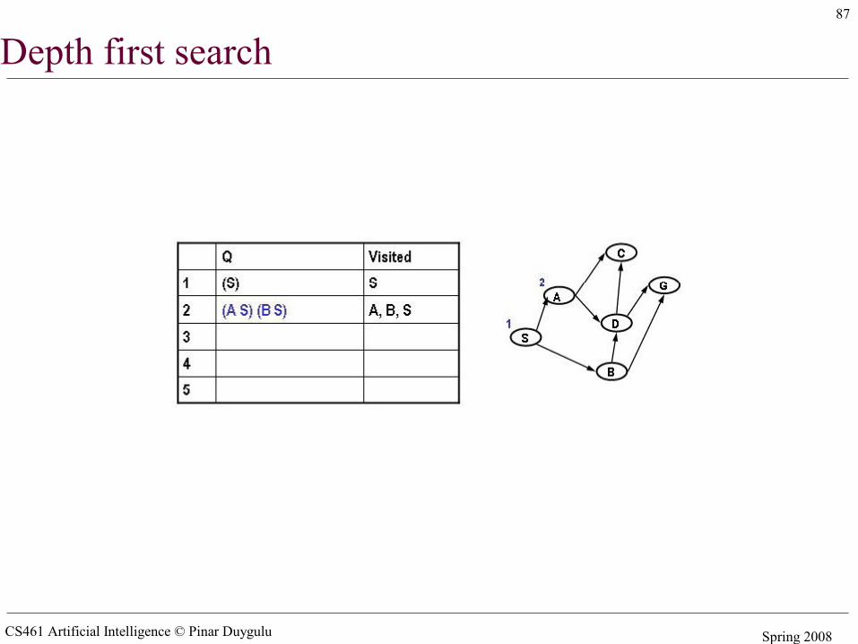
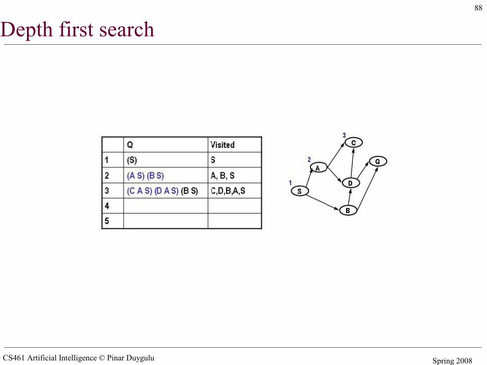
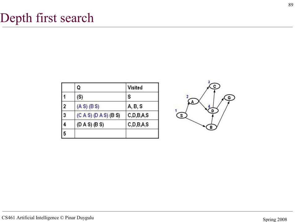
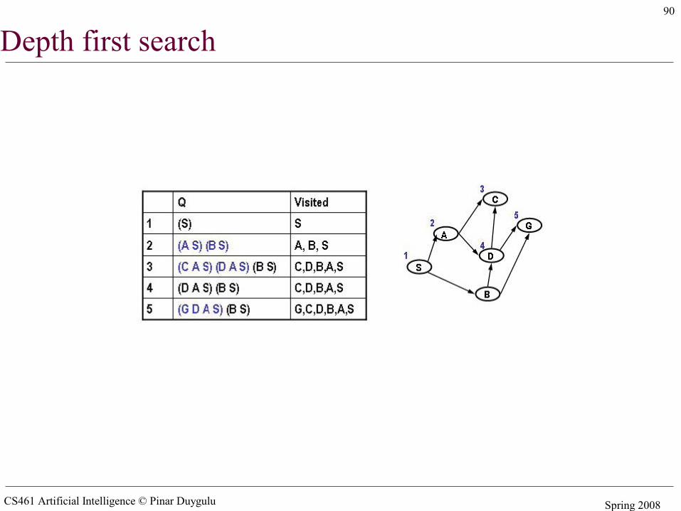
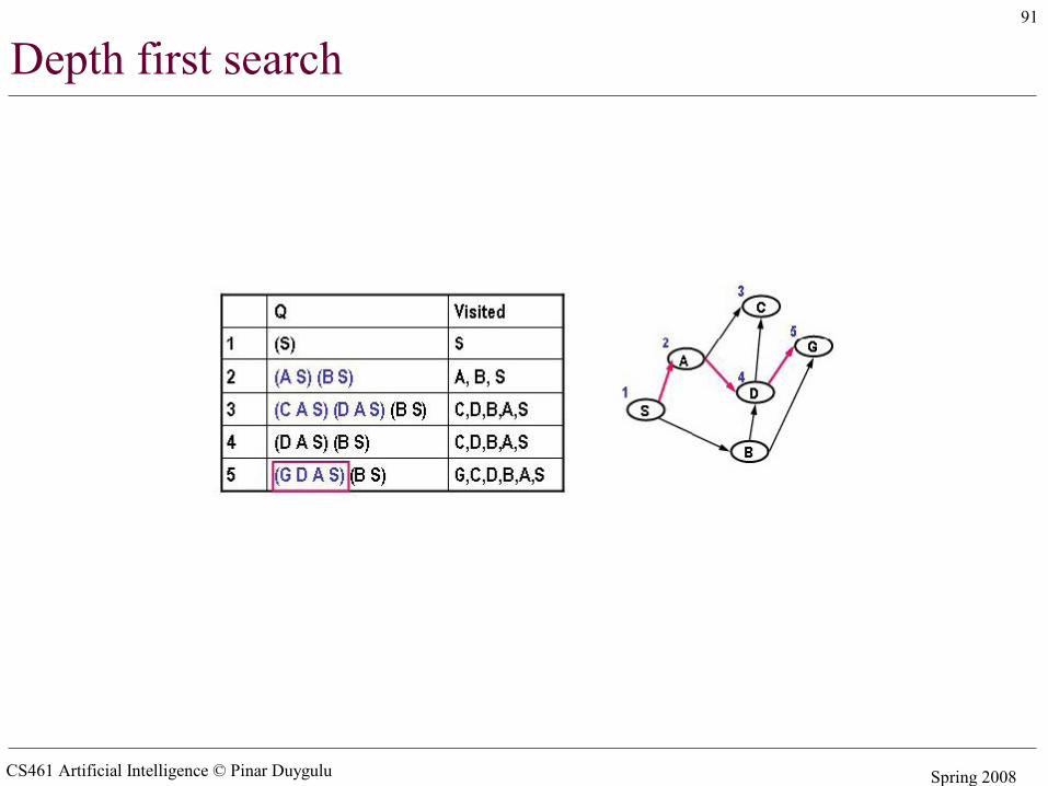
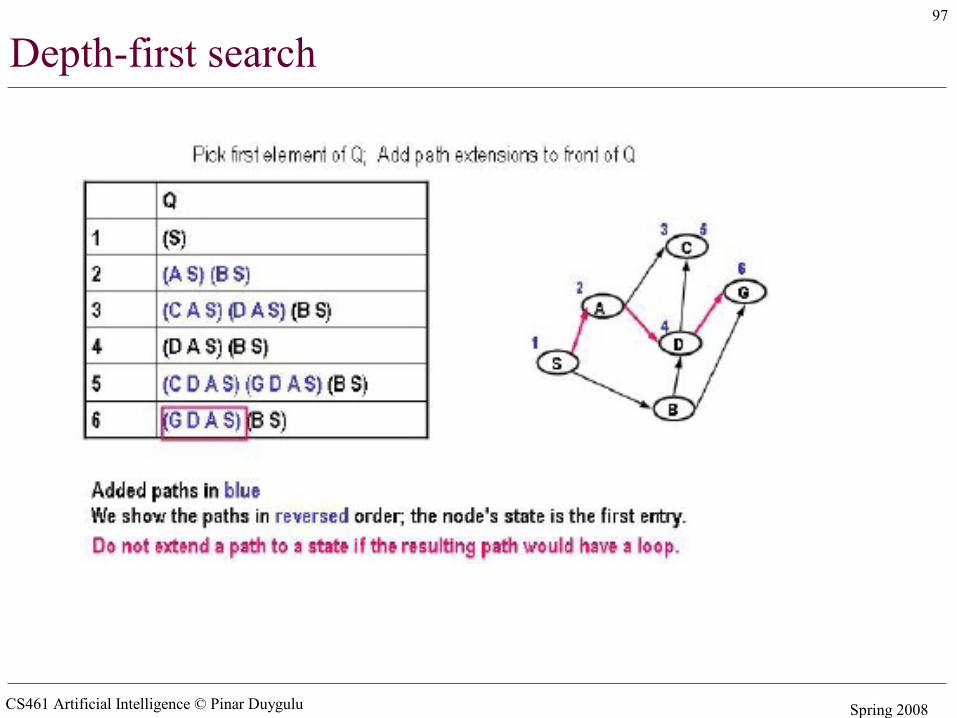
Simple search algorithms - revisited• A search node is a path from state X to the start state (e.g. X B A S)• The state of a search node is the most recent state of the path (e.g. X)• Let Q be a list of search nodes (e.g. (X B A S) (C B A S)) and S be the start state
• Algorithm
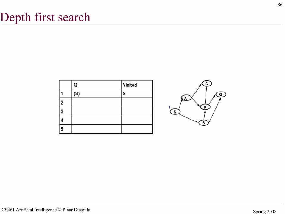
1. Initialize Q with search node (S) as only entry, set Visited = (S)2. If Q is empty, fail. Else pick some search node N from Q3. If state(N) is a goal, return N (we have reached the goal)4. Otherwise remove N from Q5. Find all the children of state(N) not in visited and create all the one-step
extensions of N to each descendant6. Add the extended paths to Q, add children of state(N) to Visited7. Go to step 2
• Critical decisions– Step2: picking N from Q– Step 6: adding extensions of N to Q
CS461 Artificial Intelligence © Pinar Duygulu Spring 2008
33
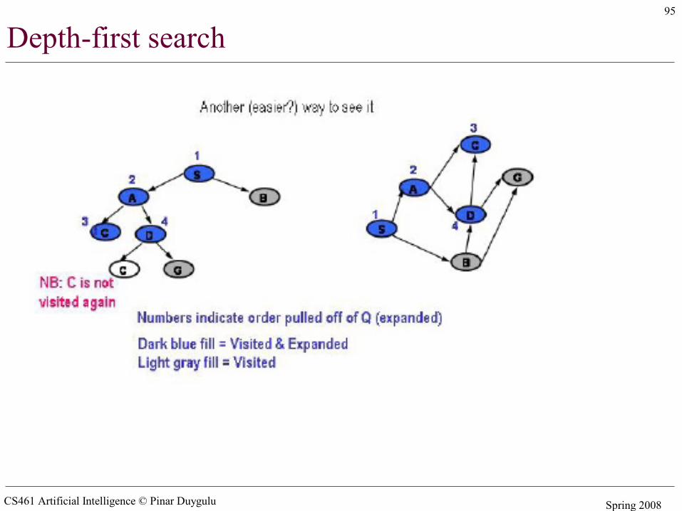
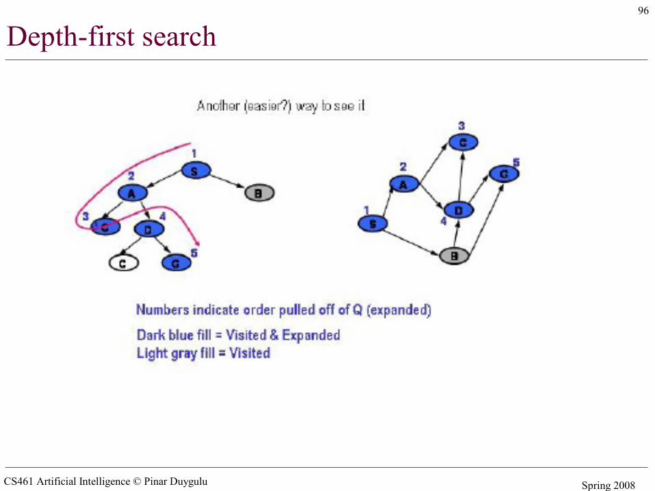
Examples: Simple search strategies
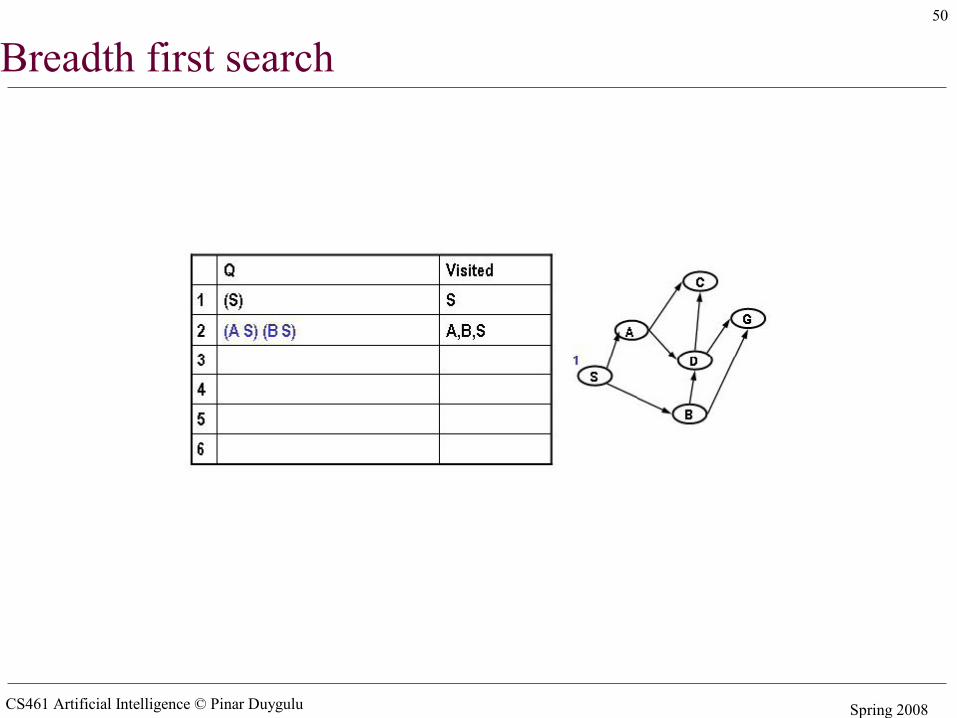
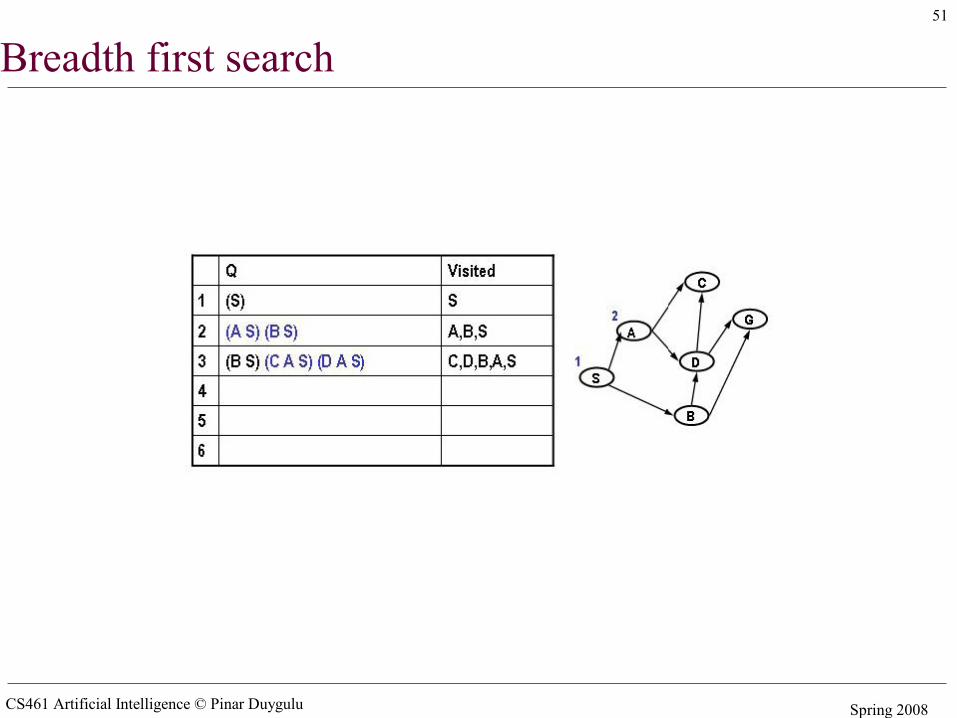
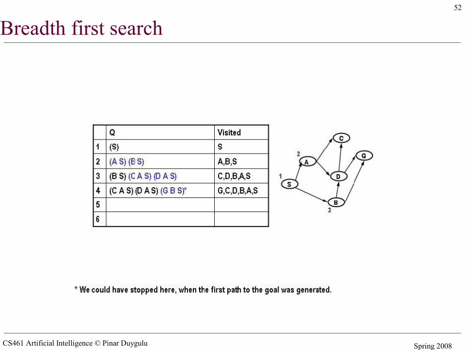
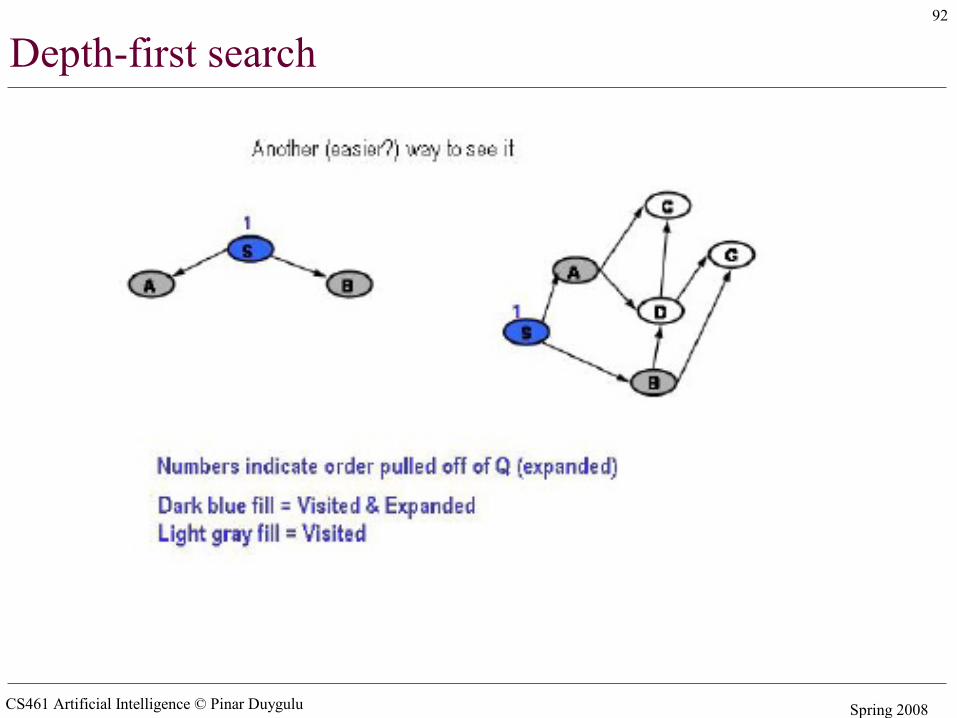
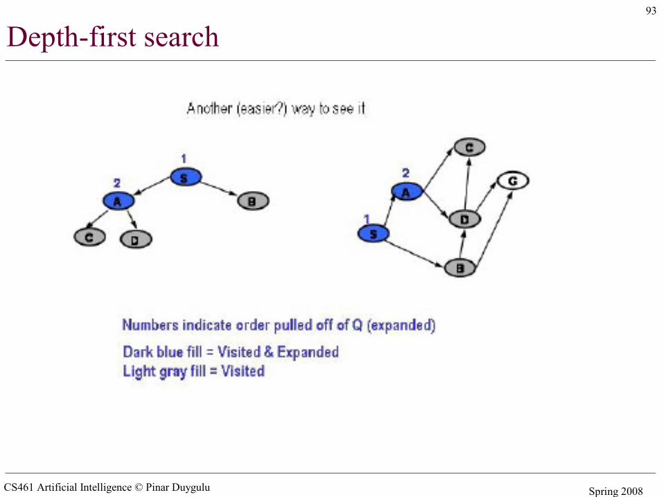
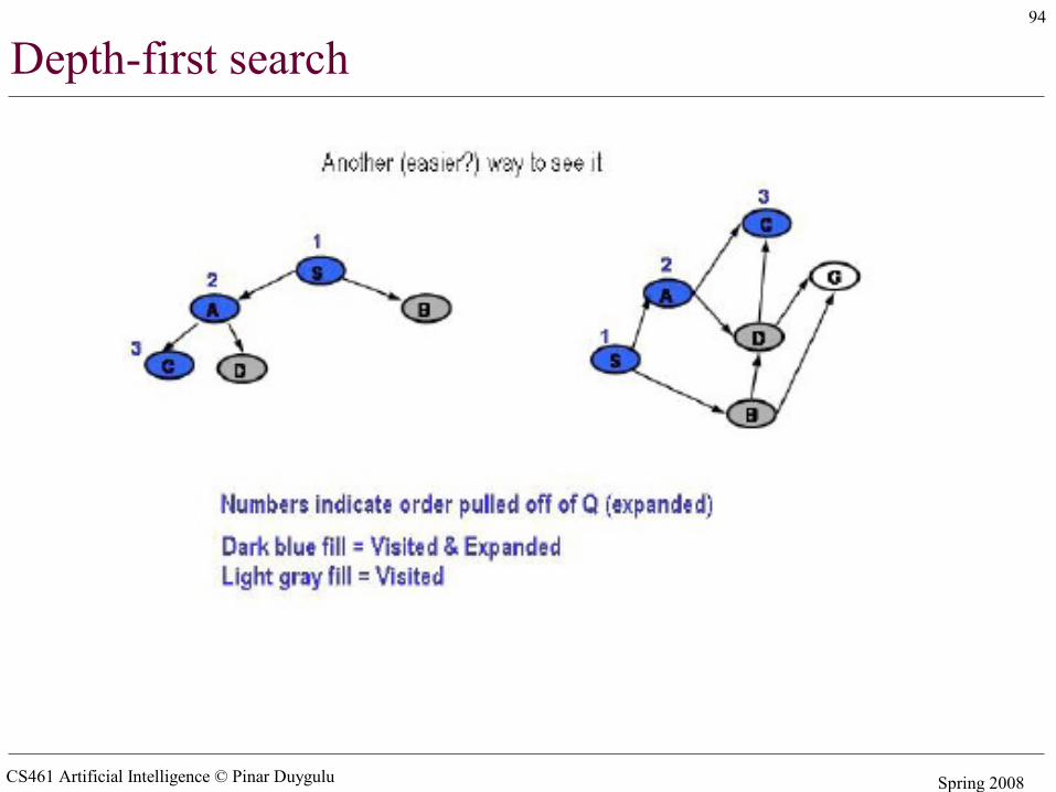
• Depth first search– Pick first element of Q– Add path extensions to front of Q
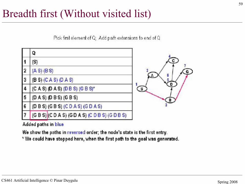
• Breadth first search– Pick first element of Q– Add path extensions to the end of Q
CS461 Artificial Intelligence © Pinar Duygulu Spring 2008
34
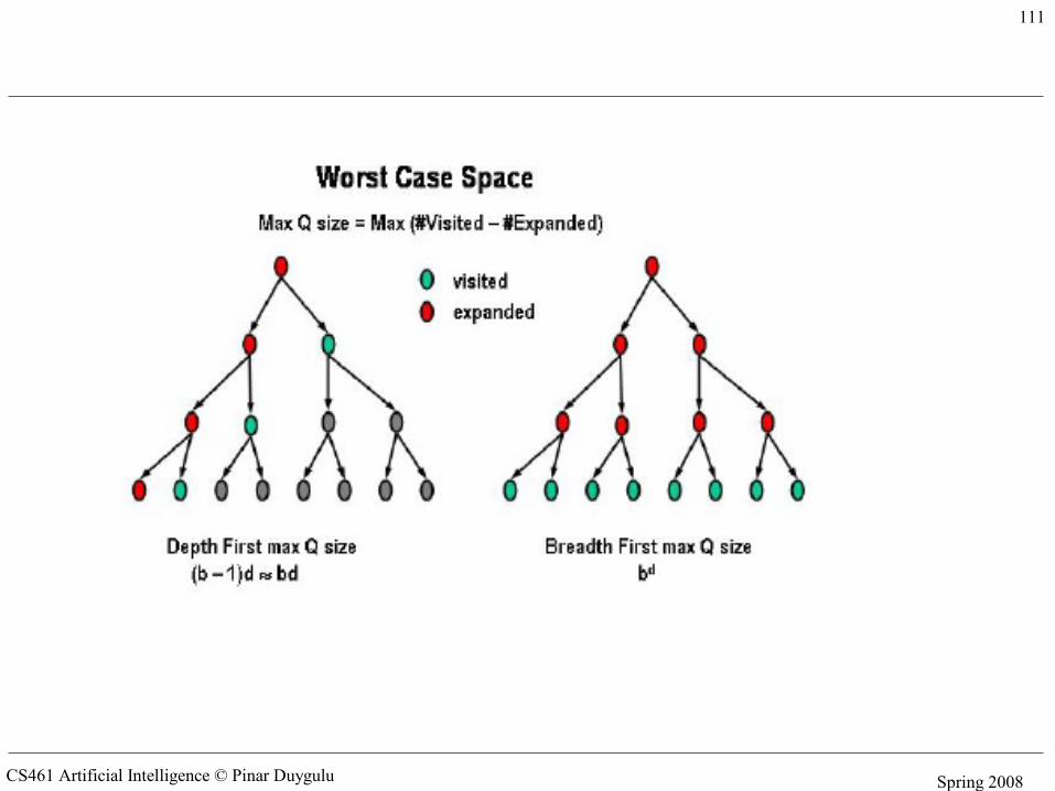
Visited versus expanded
• Visited: a state M is first visited when a path to M first gets added to Q. In general, a state is said to have been visited if it has ever shown up in a search node in Q. The intuition is that we have briefly visited them to place them on Q, but we have not yet examined them carefully
• Expanded: a state M is expanded when it is the state of a search node that is pulled off of Q. At that point, the descendants of M are visited and the path that led to M is extended to the eligible descendants. In principle, a state may be expanded multiple times. We sometimes refer to the search node that led to M as being expanded. However, once a node is expanded, we are done with it, we will not need to expand it again. In fact, we discard it from Q
CS461 Artificial Intelligence © Pinar Duygulu Spring 2008
35
Testing for the goal
• This algorithm stops (in step 3) when state(N) = G or, in general when state(N) satisfies the goal test
• We could have performed the test in step 6 as each extended path is added to Q. This would catch termination earlier
• However, performing the test in step 6 will be incorrect for the optimal searches
CS461 Artificial Intelligence © Pinar Duygulu Spring 2008
36
• Keeping track of visited states generally improves time efficiency when searching for graphs, without affecting correctness. Note, however, that substantial additional space may be required to keep track of visited states.
• If all we want to do is find a path from the start to goal, there is no advantage of adding a search node whose state is already the state of another search node
• Any state reachable from the node the second time would have been reachable from that node the first time
• Note that when using Visited, each state will only ever have at most one path to it (search node) in Q
• We’ll have to revisit this issue when we look at optimal searching
Keeping track of visited states
CS461 Artificial Intelligence © Pinar Duygulu Spring 2008
37
Implementation issues : The visit List
• Although we speak of a visited list, this is never the preferred implementation
• If the graph states are known ahead of time as an explicit set, then space is allocated in the state itself to keep a mark, which makes both adding Visited and checking if a state is Visited a constant time operation
• Alternatively, as in more common AI, if the states are generated on the fly, then a hash table may be used for efficient detection of previously visited states.
• Note that, in any case, the incremental space cost of a Visited list will be proportional to the number of states, which can be very high in some problems
CS461 Artificial Intelligence © Pinar Duygulu Spring 2008
38
Search strategies
• A search strategy is defined by picking the order of node expansion• Strategies are evaluated along the following dimensions:
– completeness: does it always find a solution if one exists?– time complexity: number of nodes generated– space complexity: maximum number of nodes in memory– optimality: does it always find a least-cost solution?
• Time and space complexity are measured in terms of – b: maximum branching factor of the search tree– d: depth of the least-cost solution– m: maximum depth of the state space (may be ∞)
CS461 Artificial Intelligence © Pinar Duygulu Spring 2008
39
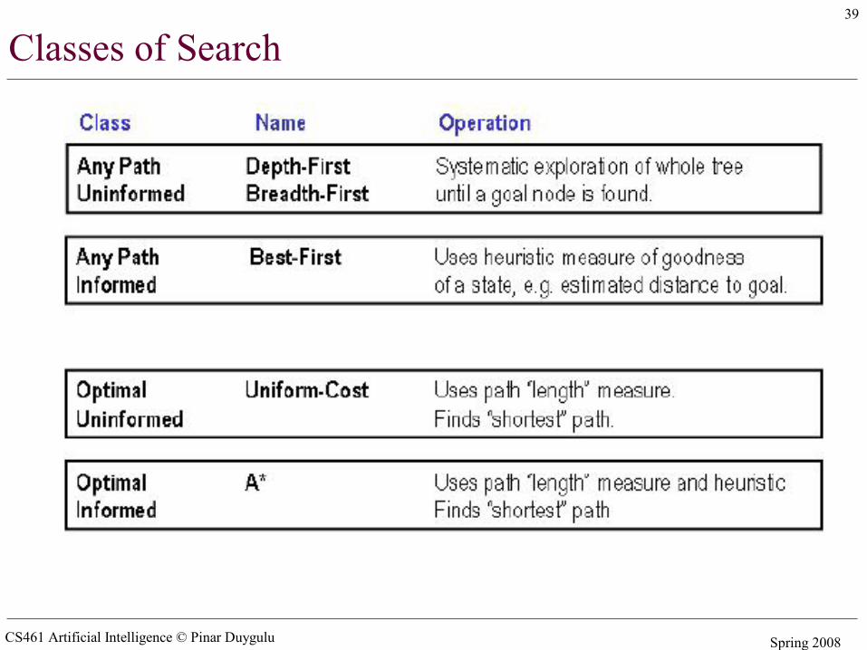
Classes of Search
CS461 Artificial Intelligence © Pinar Duygulu Spring 2008
40
Uninformed search strategies
• Uninformed search (blind search) strategies use only the information available in the problem definition
• Breadth-first search• Uniform-cost search• Depth-first search• Depth-limited search• Iterative deepening search
CS461 Artificial Intelligence © Pinar Duygulu Spring 2008
41
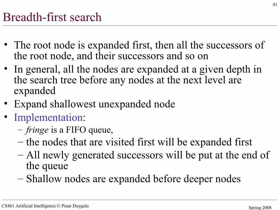
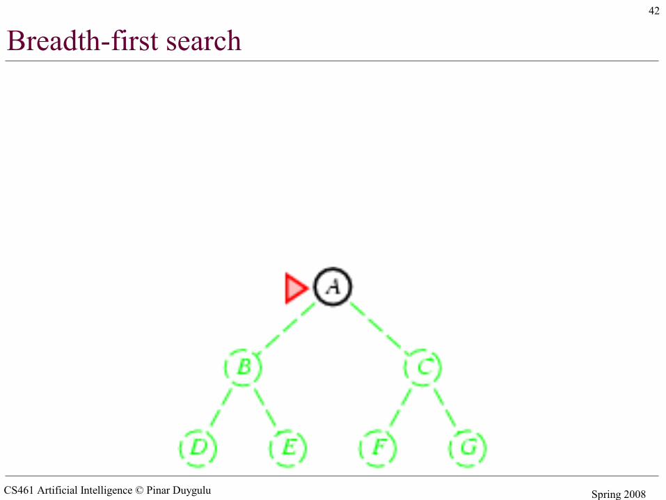
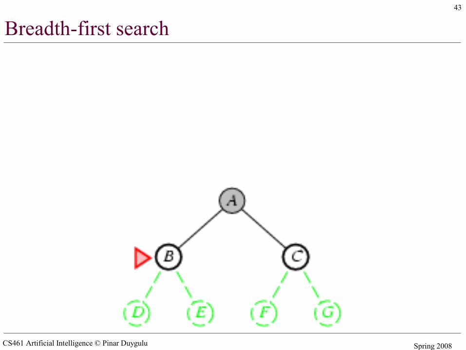
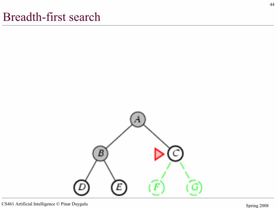
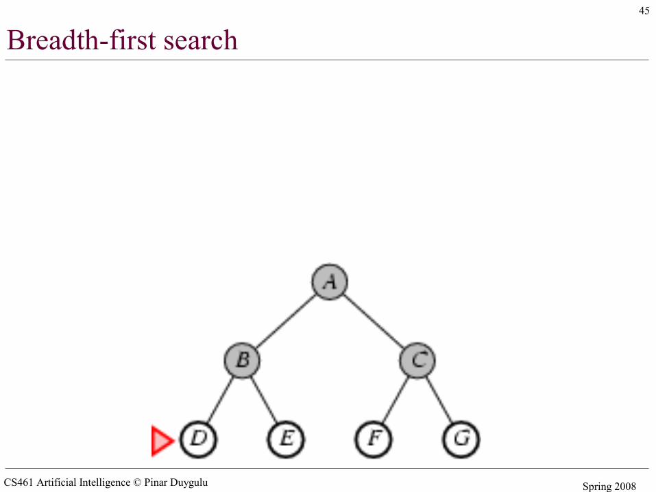
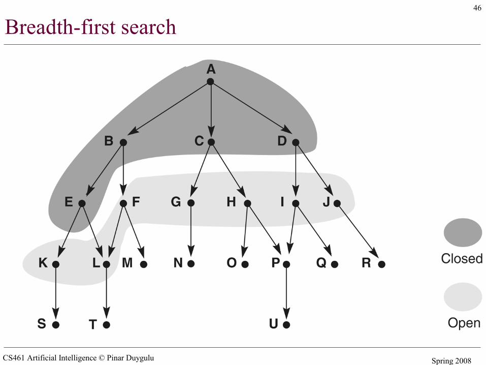
Breadth-first search
• The root node is expanded first, then all the successors of the root node, and their successors and so on
• In general, all the nodes are expanded at a given depth in the search tree before any nodes at the next level are expanded
• Expand shallowest unexpanded node• Implementation:
– fringe is a FIFO queue, – the nodes that are visited first will be expanded first– All newly generated successors will be put at the end of
the queue– Shallow nodes are expanded before deeper nodes
CS461 Artificial Intelligence © Pinar Duygulu Spring 2008
42
Breadth-first search
CS461 Artificial Intelligence © Pinar Duygulu Spring 2008
43
Breadth-first search
CS461 Artificial Intelligence © Pinar Duygulu Spring 2008
44
Breadth-first search
CS461 Artificial Intelligence © Pinar Duygulu Spring 2008
45
Breadth-first search
CS461 Artificial Intelligence © Pinar Duygulu Spring 2008
46
Breadth-first search
CS461 Artificial Intelligence © Pinar Duygulu Spring 2008
47
8-puzzle problem
CS461 Artificial Intelligence © Pinar Duygulu Spring 2008
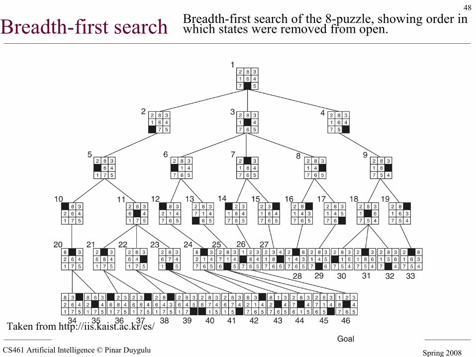
48
Breadth-first search Breadth-first search of the 8-puzzle, showing order in which states were removed from open.
Taken from http://iis.kaist.ac.kr/es/
CS461 Artificial Intelligence © Pinar Duygulu Spring 2008
49
Breadth first search
CS461 Artificial Intelligence © Pinar Duygulu Spring 2008
50
Breadth first search
CS461 Artificial Intelligence © Pinar Duygulu Spring 2008
51
Breadth first search
CS461 Artificial Intelligence © Pinar Duygulu Spring 2008
52
Breadth first search
CS461 Artificial Intelligence © Pinar Duygulu Spring 2008
53
Breadth first search

CS461 Artificial Intelligence © Pinar Duygulu Spring 2008
54
Breadth first search
CS461 Artificial Intelligence © Pinar Duygulu Spring 2008
55
Breadth first search
CS461 Artificial Intelligence © Pinar Duygulu Spring 2008
56
Breadth first search
CS461 Artificial Intelligence © Pinar Duygulu Spring 2008
57
Breadth first search
CS461 Artificial Intelligence © Pinar Duygulu Spring 2008
58
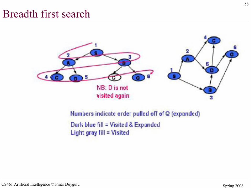
Breadth first search
CS461 Artificial Intelligence © Pinar Duygulu Spring 2008
59
Breadth first (Without visited list)
CS461 Artificial Intelligence © Pinar Duygulu Spring 2008
60
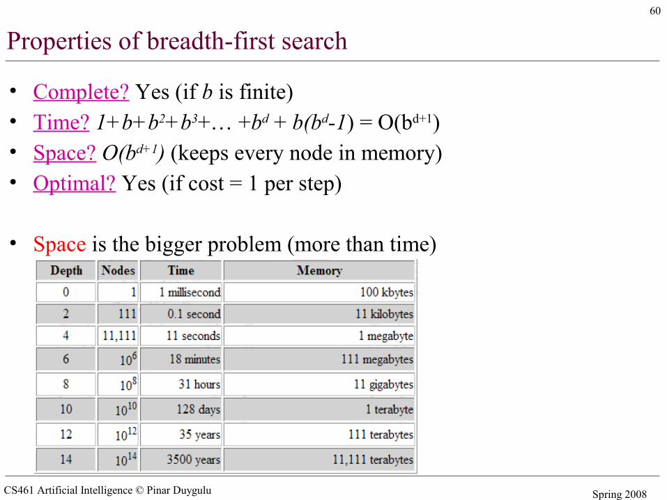
Properties of breadth-first search
• Complete? Yes (if b is finite)• Time? 1+b+b2+b3+… +bd + b(bd-1) = O(bd+1)• Space? O(bd+1) (keeps every node in memory)• Optimal? Yes (if cost = 1 per step)
• Space is the bigger problem (more than time)
CS461 Artificial Intelligence © Pinar Duygulu Spring 2008
61
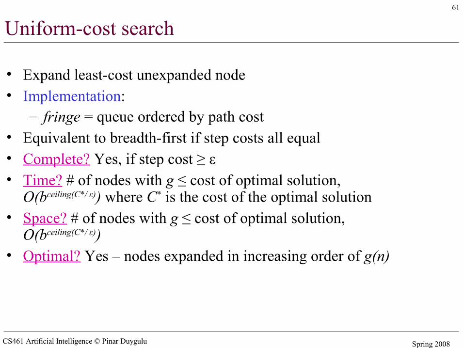
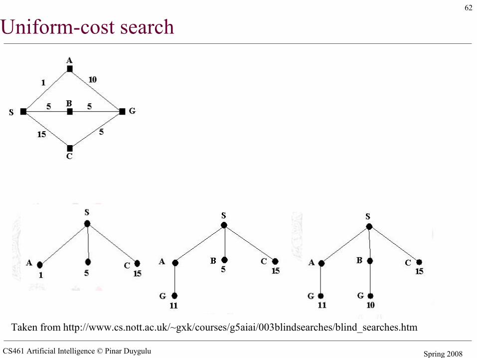
Uniform-cost search
• Expand least-cost unexpanded node• Implementation:
– fringe = queue ordered by path cost• Equivalent to breadth-first if step costs all equal• Complete? Yes, if step cost ≥ ε• Time? # of nodes with g ≤ cost of optimal solution,
O(bceiling(C*/ ε)) where C* is the cost of the optimal solution• Space? # of nodes with g ≤ cost of optimal solution,
O(bceiling(C*/ ε))• Optimal? Yes – nodes expanded in increasing order of g(n)
CS461 Artificial Intelligence © Pinar Duygulu Spring 2008
62
Uniform-cost search
Taken from http://www.cs.nott.ac.uk/~gxk/courses/g5aiai/003blindsearches/blind_searches.htm
CS461 Artificial Intelligence © Pinar Duygulu Spring 2008
63
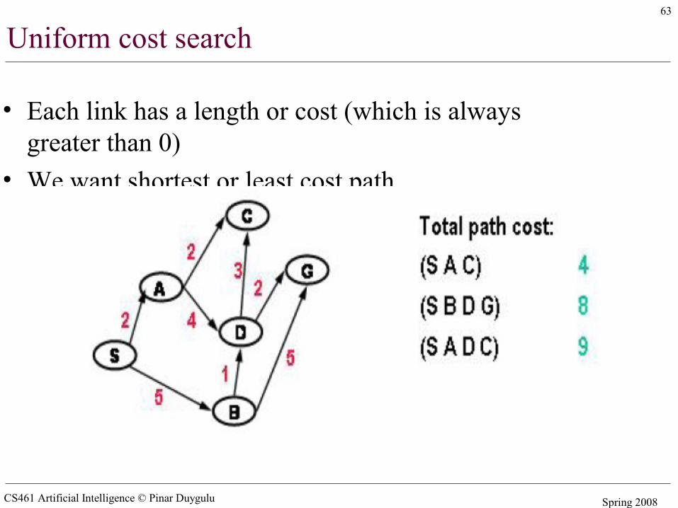
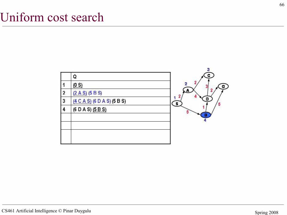
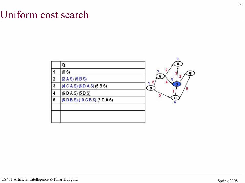
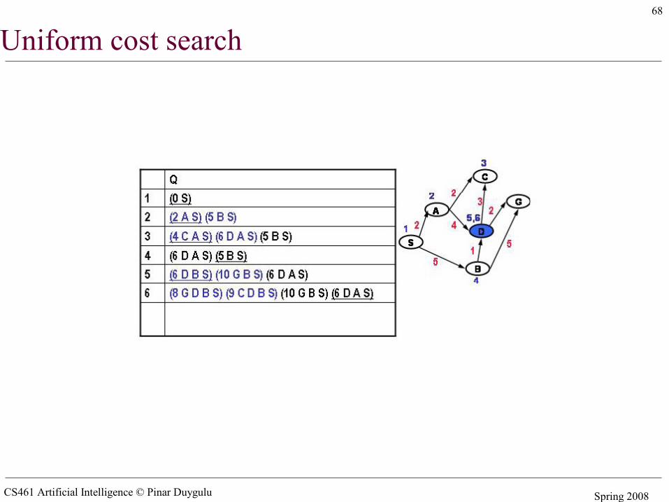
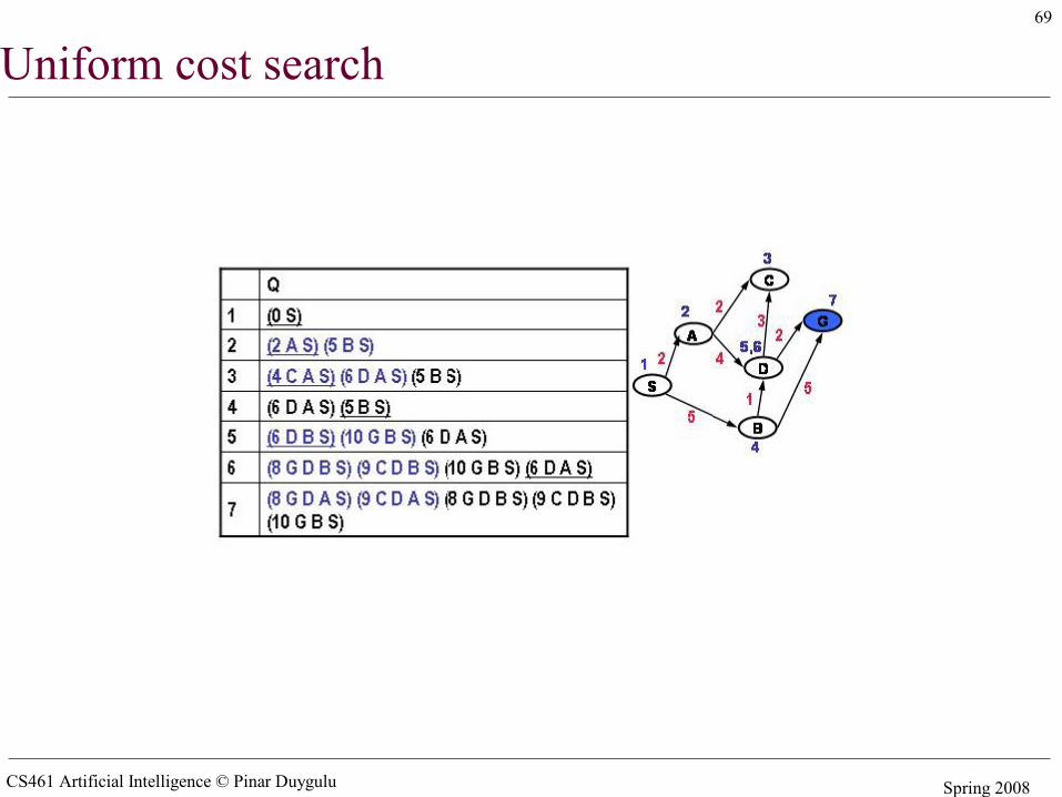
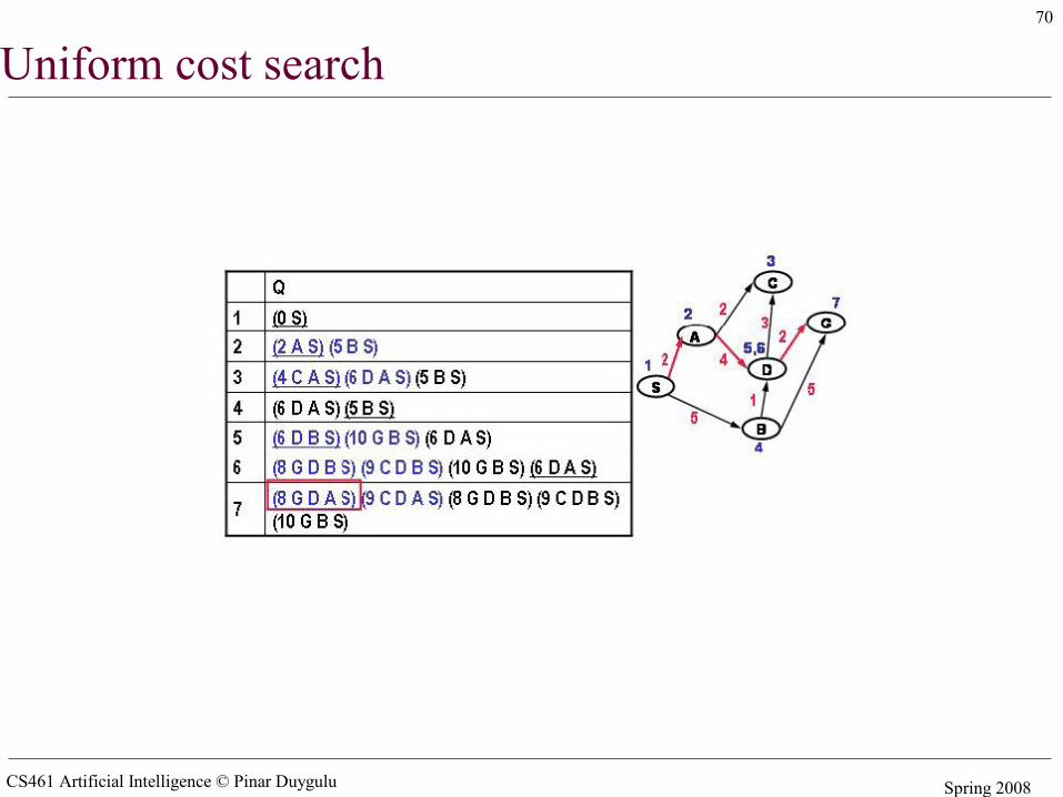
Uniform cost search
• Each link has a length or cost (which is always greater than 0)
• We want shortest or least cost path
CS461 Artificial Intelligence © Pinar Duygulu Spring 2008
64
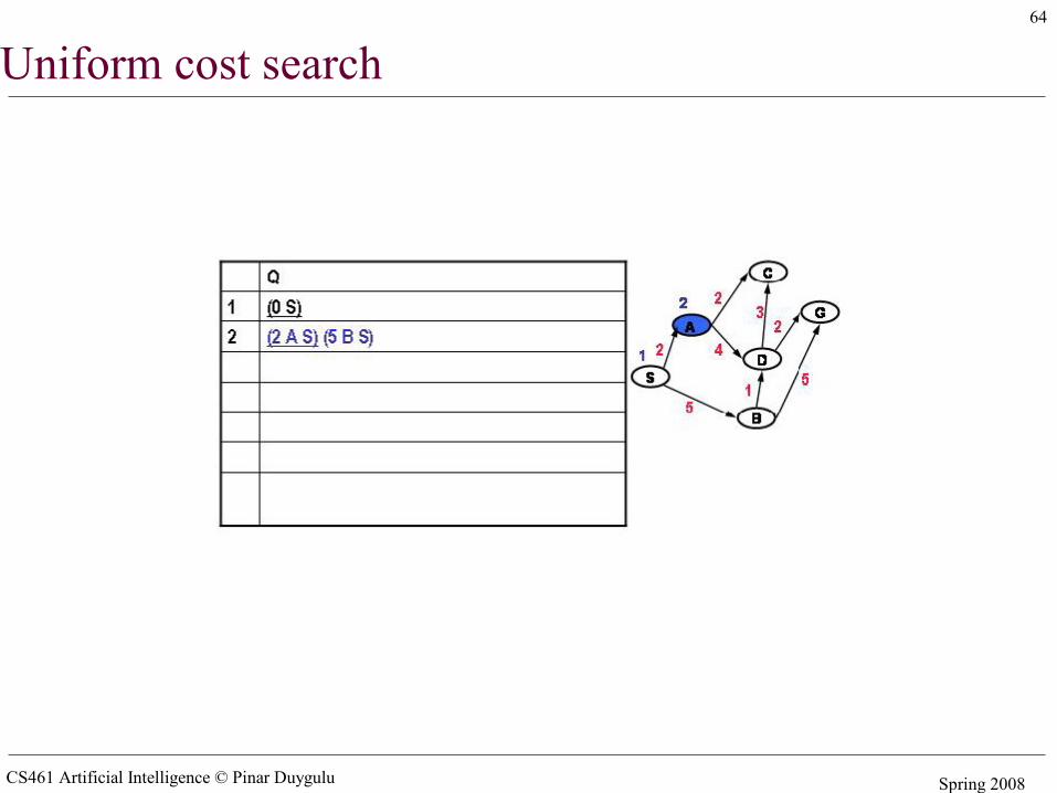
Uniform cost search
CS461 Artificial Intelligence © Pinar Duygulu Spring 2008
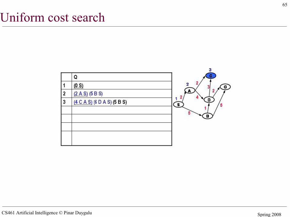
65
Uniform cost search
CS461 Artificial Intelligence © Pinar Duygulu Spring 2008
66
Uniform cost search
CS461 Artificial Intelligence © Pinar Duygulu Spring 2008
67
Uniform cost search
CS461 Artificial Intelligence © Pinar Duygulu Spring 2008
68
Uniform cost search
CS461 Artificial Intelligence © Pinar Duygulu Spring 2008
69
Uniform cost search
CS461 Artificial Intelligence © Pinar Duygulu Spring 2008
70
Uniform cost search
CS461 Artificial Intelligence © Pinar Duygulu Spring 2008
71
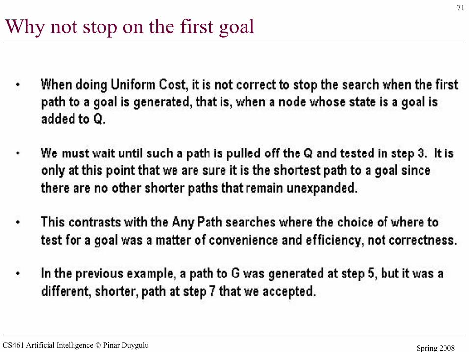
Why not stop on the first goal
CS461 Artificial Intelligence © Pinar Duygulu Spring 2008
72
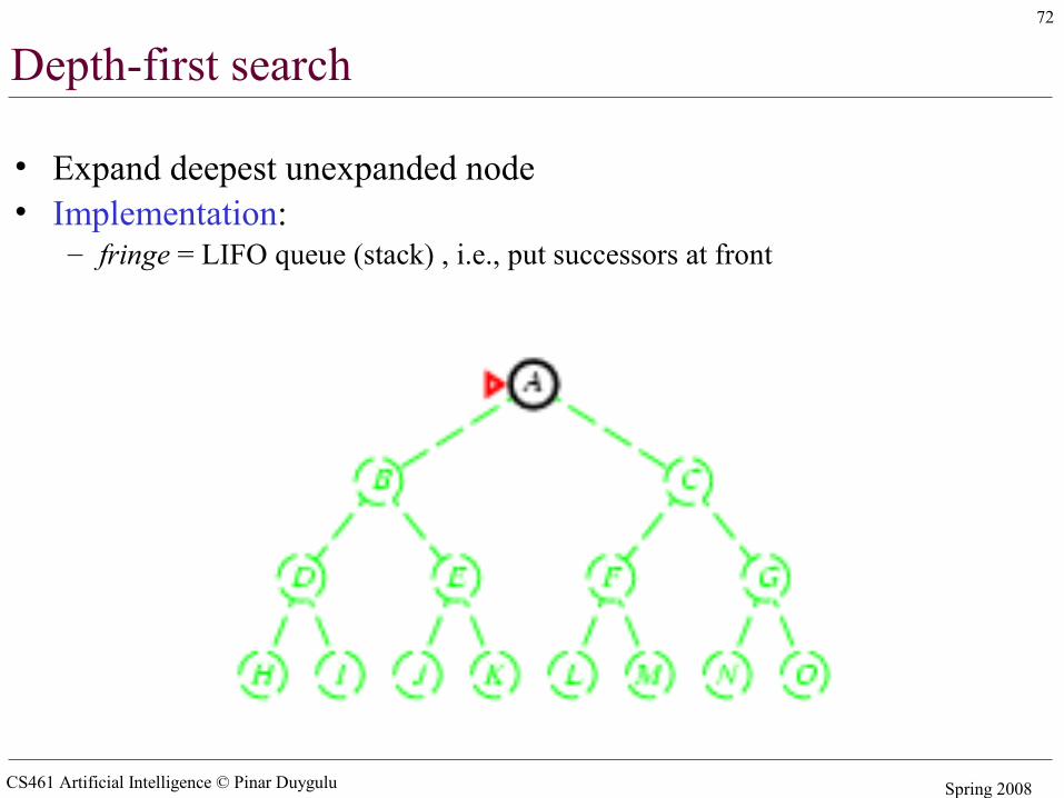
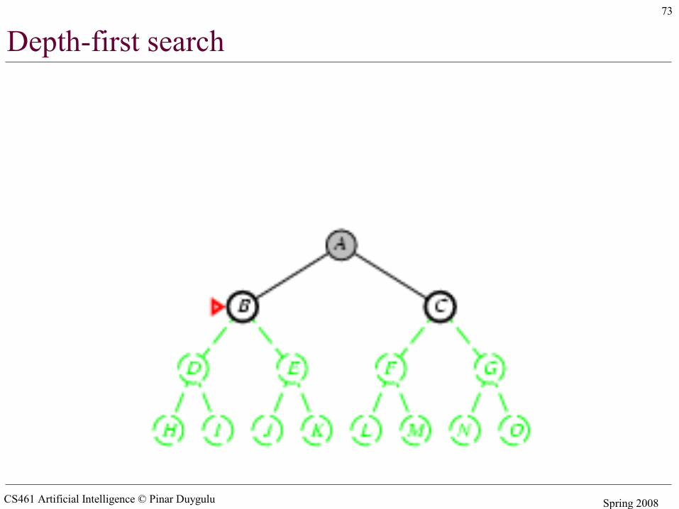
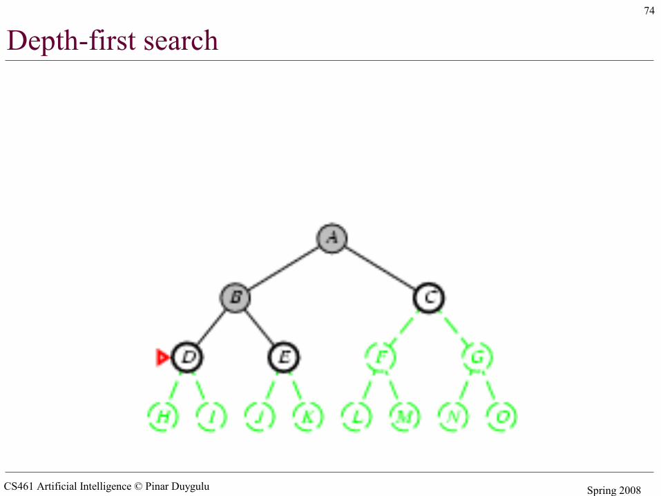
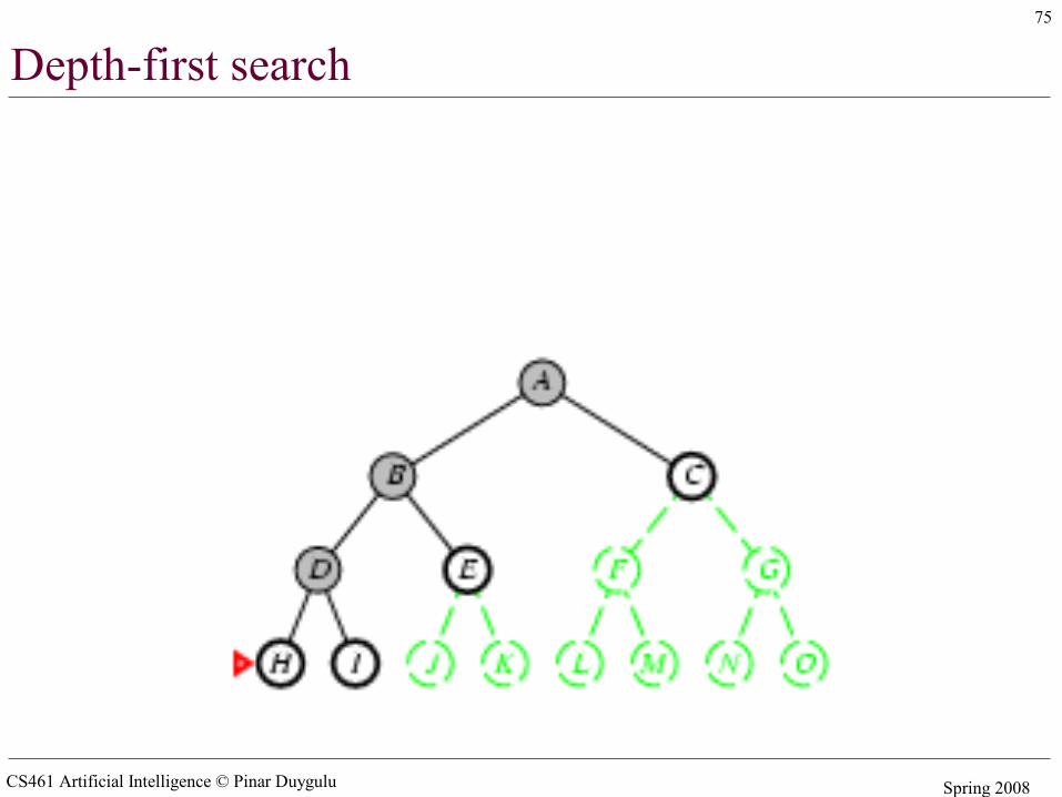
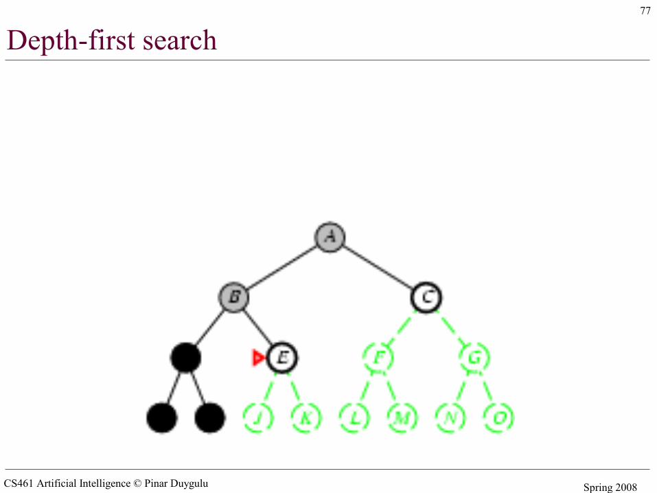
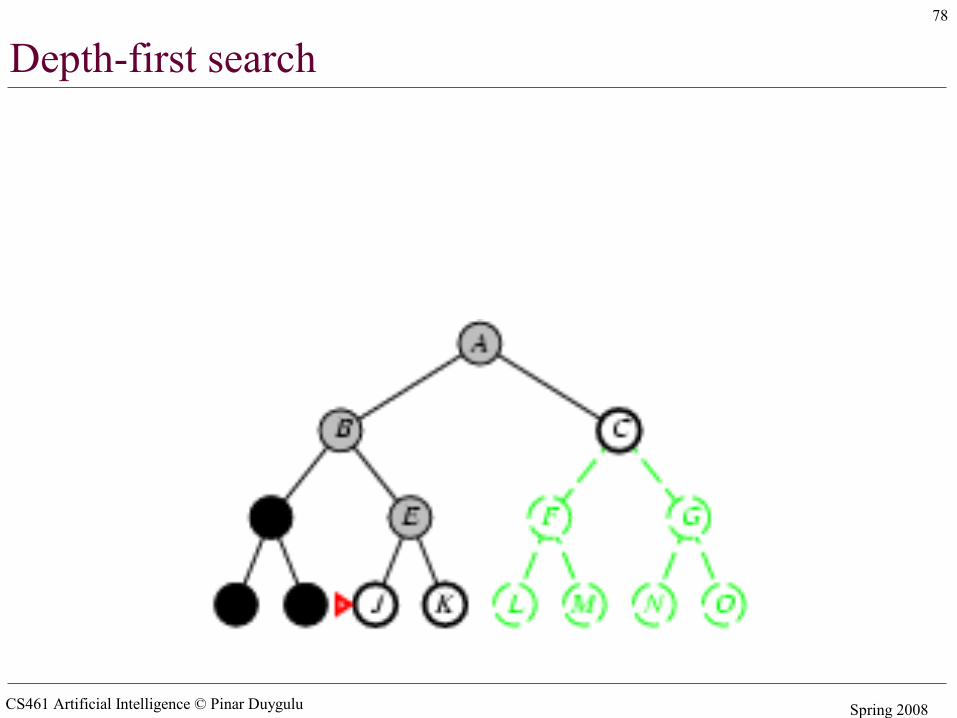
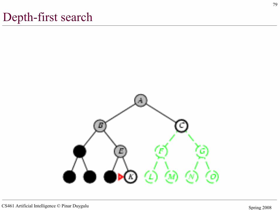
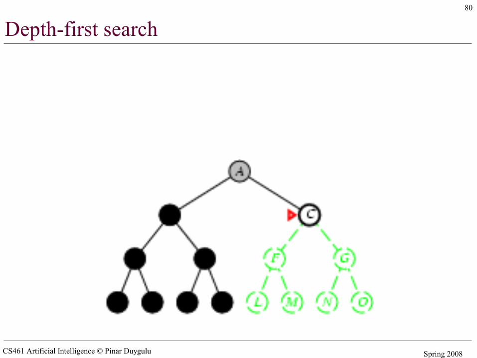
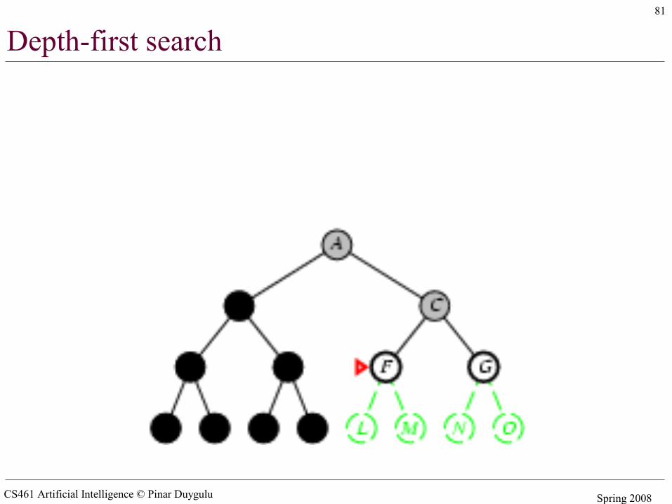
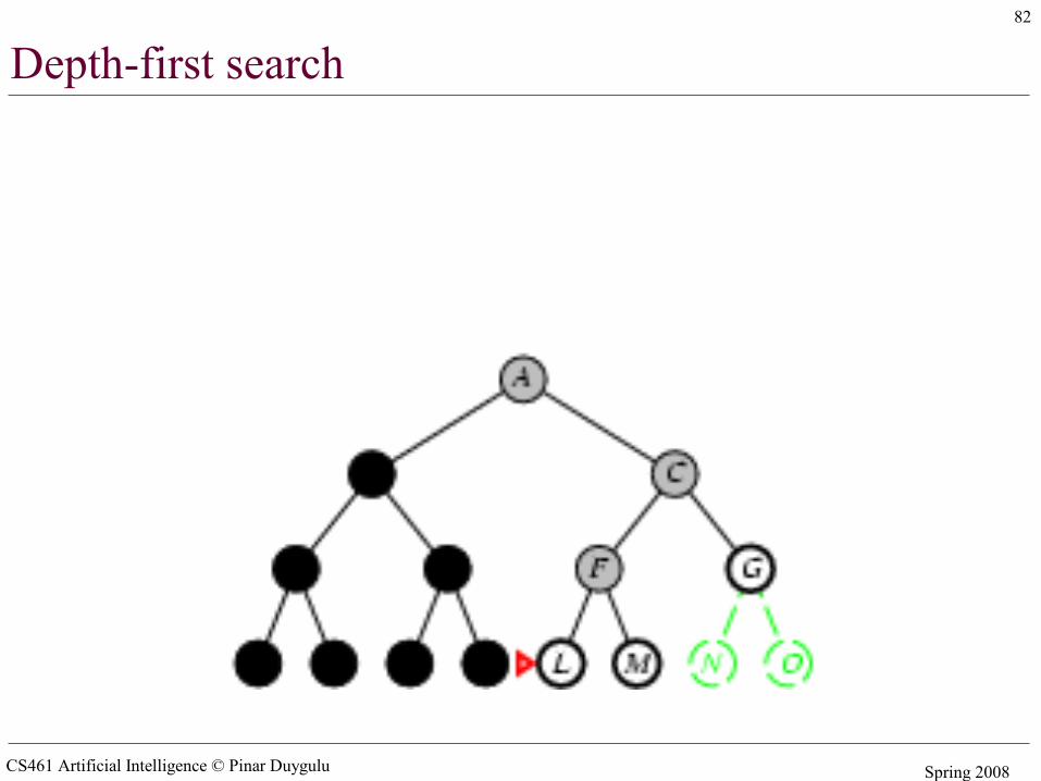
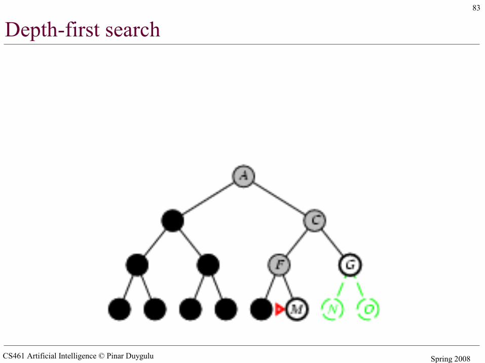
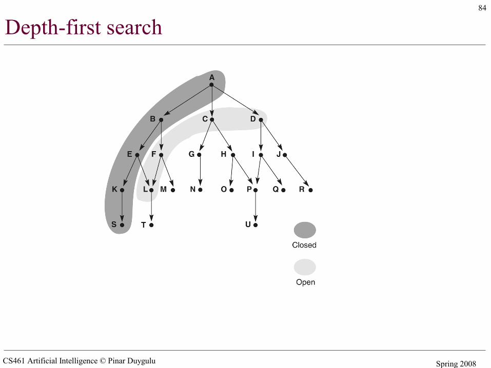
Depth-first search
• Expand deepest unexpanded node• Implementation:
– fringe = LIFO queue (stack) , i.e., put successors at front
CS461 Artificial Intelligence © Pinar Duygulu Spring 2008
73
Depth-first search
CS461 Artificial Intelligence © Pinar Duygulu Spring 2008
74
Depth-first search
CS461 Artificial Intelligence © Pinar Duygulu Spring 2008
75
Depth-first search

CS461 Artificial Intelligence © Pinar Duygulu Spring 2008
76
Depth-first search
CS461 Artificial Intelligence © Pinar Duygulu Spring 2008
77
Depth-first search
CS461 Artificial Intelligence © Pinar Duygulu Spring 2008
78
Depth-first search
CS461 Artificial Intelligence © Pinar Duygulu Spring 2008
79
Depth-first search
CS461 Artificial Intelligence © Pinar Duygulu Spring 2008
80
Depth-first search
CS461 Artificial Intelligence © Pinar Duygulu Spring 2008
81
Depth-first search
CS461 Artificial Intelligence © Pinar Duygulu Spring 2008
82
Depth-first search
CS461 Artificial Intelligence © Pinar Duygulu Spring 2008
83
Depth-first search
CS461 Artificial Intelligence © Pinar Duygulu Spring 2008
84
Depth-first search
CS461 Artificial Intelligence © Pinar Duygulu Spring 2008
85
Depth first search
CS461 Artificial Intelligence © Pinar Duygulu Spring 2008
86
Depth first search
CS461 Artificial Intelligence © Pinar Duygulu Spring 2008
87
Depth first search
CS461 Artificial Intelligence © Pinar Duygulu Spring 2008
88
Depth first search
CS461 Artificial Intelligence © Pinar Duygulu Spring 2008
89
Depth first search
CS461 Artificial Intelligence © Pinar Duygulu Spring 2008
90
Depth first search
CS461 Artificial Intelligence © Pinar Duygulu Spring 2008
91
Depth first search
CS461 Artificial Intelligence © Pinar Duygulu Spring 2008
92
Depth-first search
CS461 Artificial Intelligence © Pinar Duygulu Spring 2008
93
Depth-first search
CS461 Artificial Intelligence © Pinar Duygulu Spring 2008
94
Depth-first search
CS461 Artificial Intelligence © Pinar Duygulu Spring 2008
95
Depth-first search
CS461 Artificial Intelligence © Pinar Duygulu Spring 2008
96
Depth-first search
CS461 Artificial Intelligence © Pinar Duygulu Spring 2008
97
Depth-first search
CS461 Artificial Intelligence © Pinar Duygulu Spring 2008
98
Properties of depth-first search
• Complete? No: fails in infinite-depth spaces, spaces with loops– Modify to avoid repeated states along path
complete in finite spaces• Time? O(bm): terrible if m is much larger than d
– but if solutions are dense, may be much faster than breadth-first
• Space? O(bm), i.e., linear space!• Optimal? No
CS461 Artificial Intelligence © Pinar Duygulu Spring 2008
99
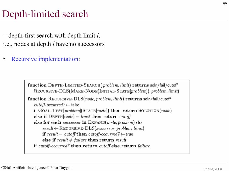
Depth-limited search
= depth-first search with depth limit l,i.e., nodes at depth l have no successors
• Recursive implementation:
CS461 Artificial Intelligence © Pinar Duygulu Spring 2008
100
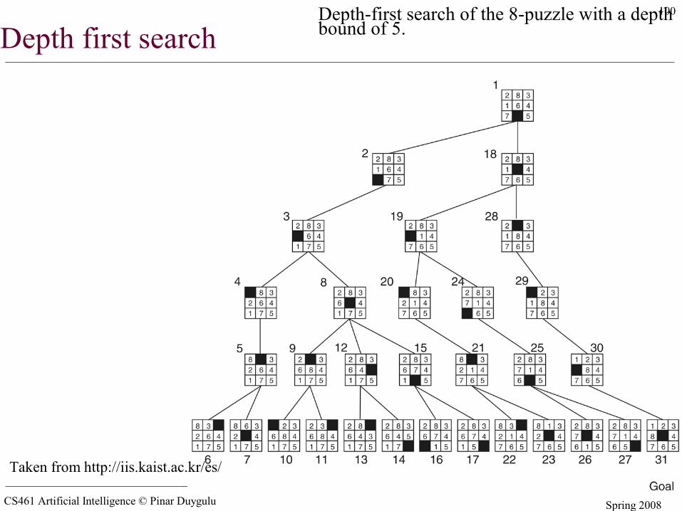
Depth first searchDepth-first search of the 8-puzzle with a depth bound of 5.
Taken from http://iis.kaist.ac.kr/es/
CS461 Artificial Intelligence © Pinar Duygulu Spring 2008
101
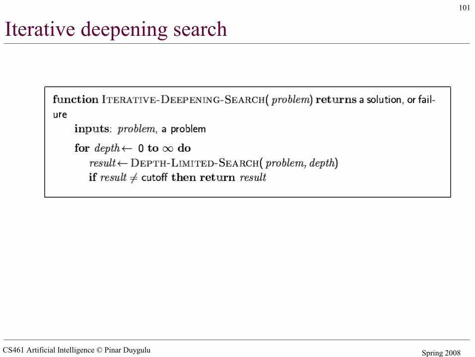
Iterative deepening search
CS461 Artificial Intelligence © Pinar Duygulu Spring 2008
102
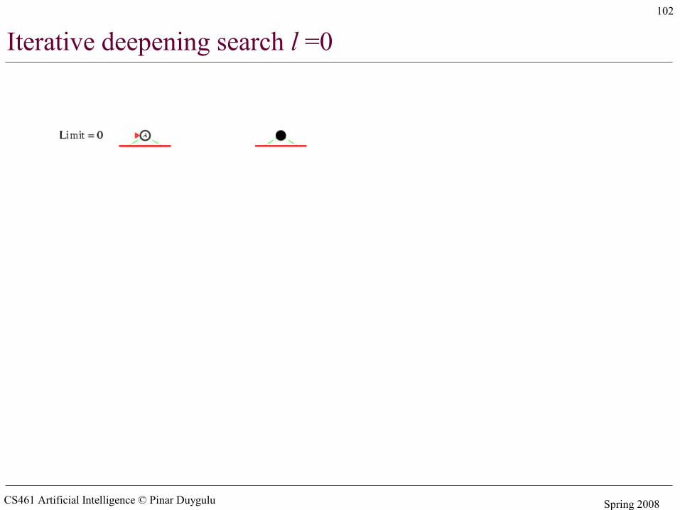
Iterative deepening search l =0
CS461 Artificial Intelligence © Pinar Duygulu Spring 2008
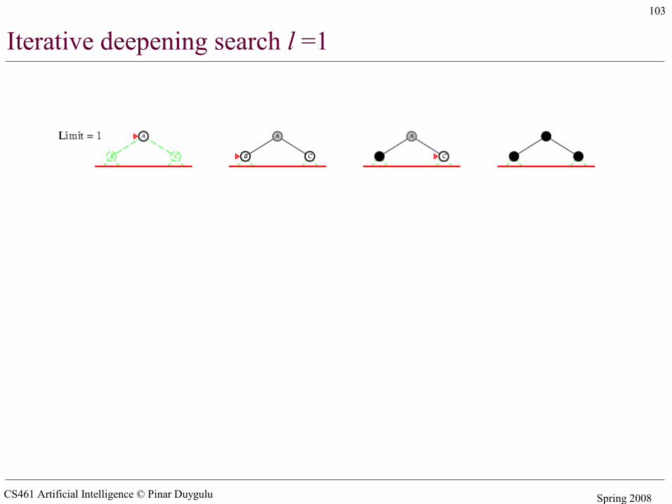
103
Iterative deepening search l =1
CS461 Artificial Intelligence © Pinar Duygulu Spring 2008
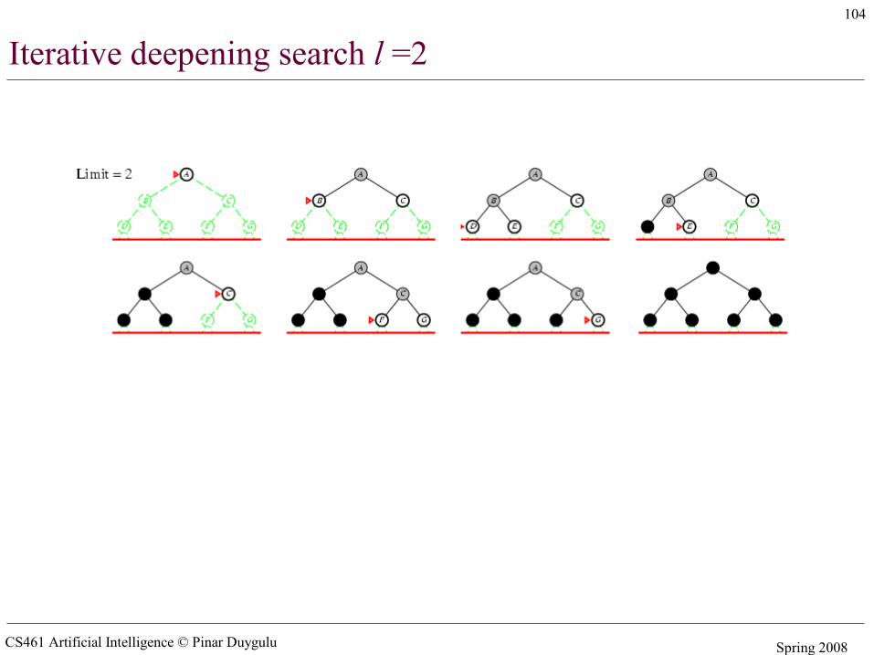
104
Iterative deepening search l =2
CS461 Artificial Intelligence © Pinar Duygulu Spring 2008
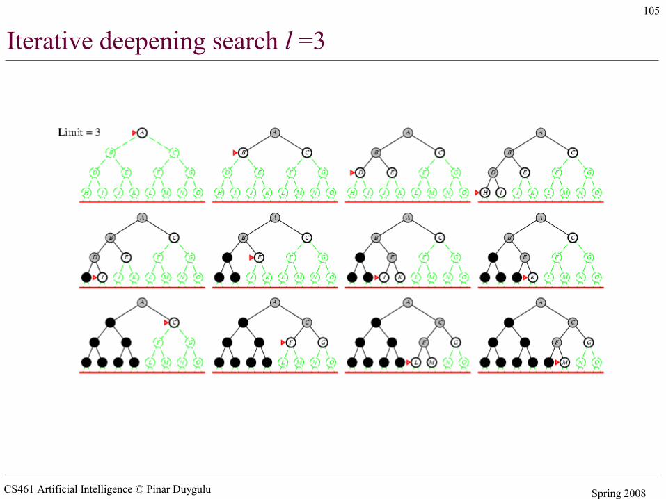
105
Iterative deepening search l =3
CS461 Artificial Intelligence © Pinar Duygulu Spring 2008
106
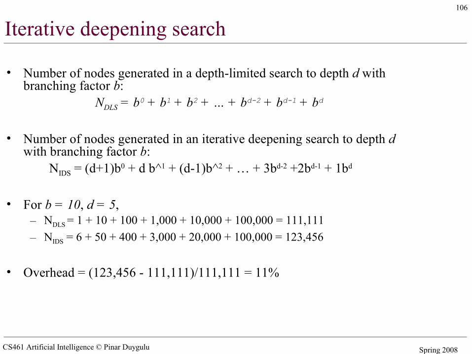
Iterative deepening search
• Number of nodes generated in a depth-limited search to depth d with branching factor b:
NDLS = b0 + b1 + b2 + … + bd-2 + bd-1 + bd
• Number of nodes generated in an iterative deepening search to depth d with branching factor b:
NIDS = (d+1)b0 + d b^1 + (d-1)b^2 + … + 3bd-2 +2bd-1 + 1bd
• For b = 10, d = 5,– NDLS = 1 + 10 + 100 + 1,000 + 10,000 + 100,000 = 111,111– NIDS = 6 + 50 + 400 + 3,000 + 20,000 + 100,000 = 123,456
• Overhead = (123,456 - 111,111)/111,111 = 11%
CS461 Artificial Intelligence © Pinar Duygulu Spring 2008
107
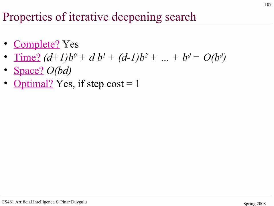
Properties of iterative deepening search
• Complete? Yes• Time? (d+1)b0 + d b1 + (d-1)b2 + … + bd = O(bd)• Space? O(bd)• Optimal? Yes, if step cost = 1
CS461 Artificial Intelligence © Pinar Duygulu Spring 2008
108
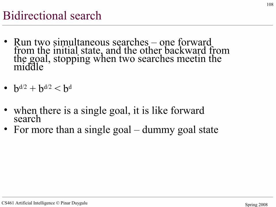
Bidirectional search
• Run two simultaneous searches – one forward from the initial state, and the other backward from the goal, stopping when two searches meetin the middle
• bd/2 + bd/2 < bd
• when there is a single goal, it is like forward search
• For more than a single goal – dummy goal state
CS461 Artificial Intelligence © Pinar Duygulu Spring 2008
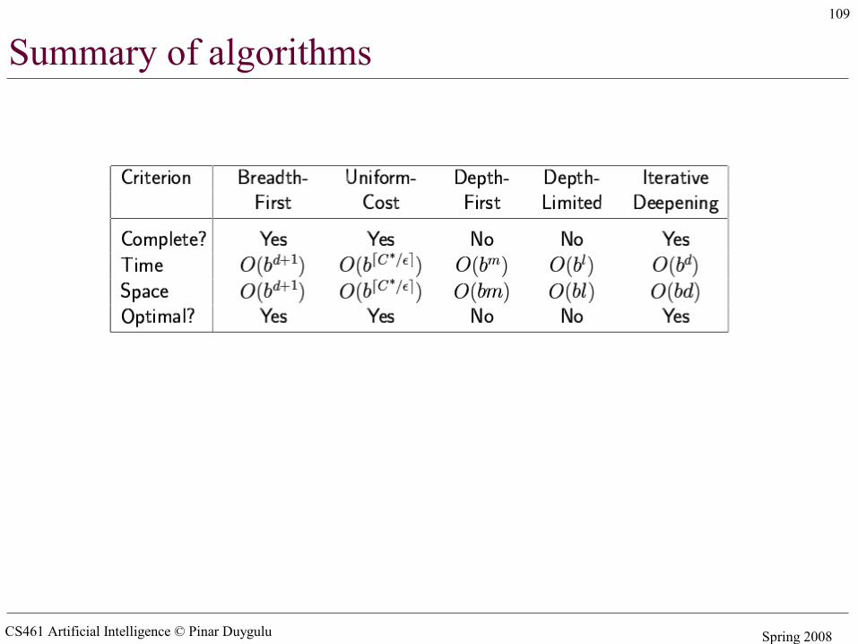
109
Summary of algorithms
CS461 Artificial Intelligence © Pinar Duygulu Spring 2008
110
CS461 Artificial Intelligence © Pinar Duygulu Spring 2008
111
CS461 Artificial Intelligence © Pinar Duygulu Spring 2008
112
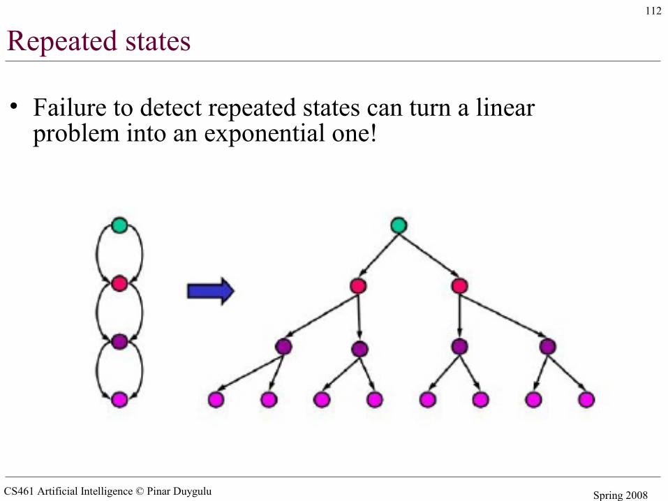
Repeated states
• Failure to detect repeated states can turn a linear problem into an exponential one!
CS461 Artificial Intelligence © Pinar Duygulu Spring 2008
113
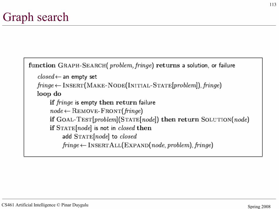
Graph search
CS461 Artificial Intelligence © Pinar Duygulu Spring 2008
114
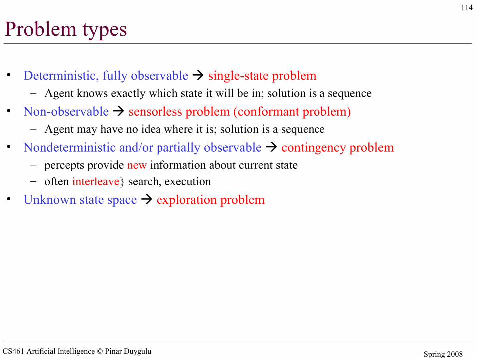
Problem types
• Deterministic, fully observable single-state problem– Agent knows exactly which state it will be in; solution is a sequence
• Non-observable sensorless problem (conformant problem)– Agent may have no idea where it is; solution is a sequence
• Nondeterministic and/or partially observable contingency problem– percepts provide new information about current state– often interleave} search, execution
• Unknown state space exploration problem
CS461 Artificial Intelligence © Pinar Duygulu Spring 2008
115
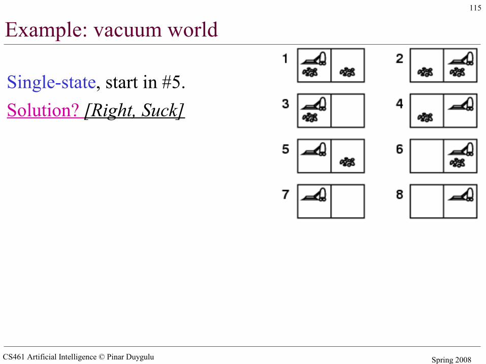
Example: vacuum world
Single-state, start in #5. Solution? [Right, Suck]
CS461 Artificial Intelligence © Pinar Duygulu Spring 2008
116
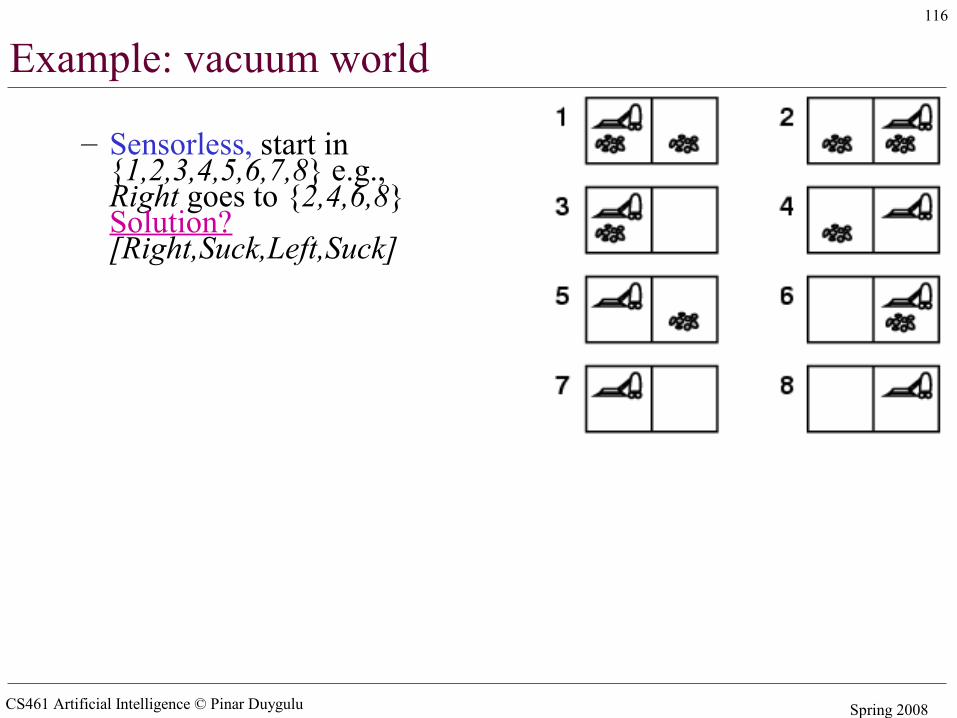
Example: vacuum world
– Sensorless, start in {1,2,3,4,5,6,7,8} e.g., Right goes to {2,4,6,8} Solution? [Right,Suck,Left,Suck]
CS461 Artificial Intelligence © Pinar Duygulu Spring 2008
117
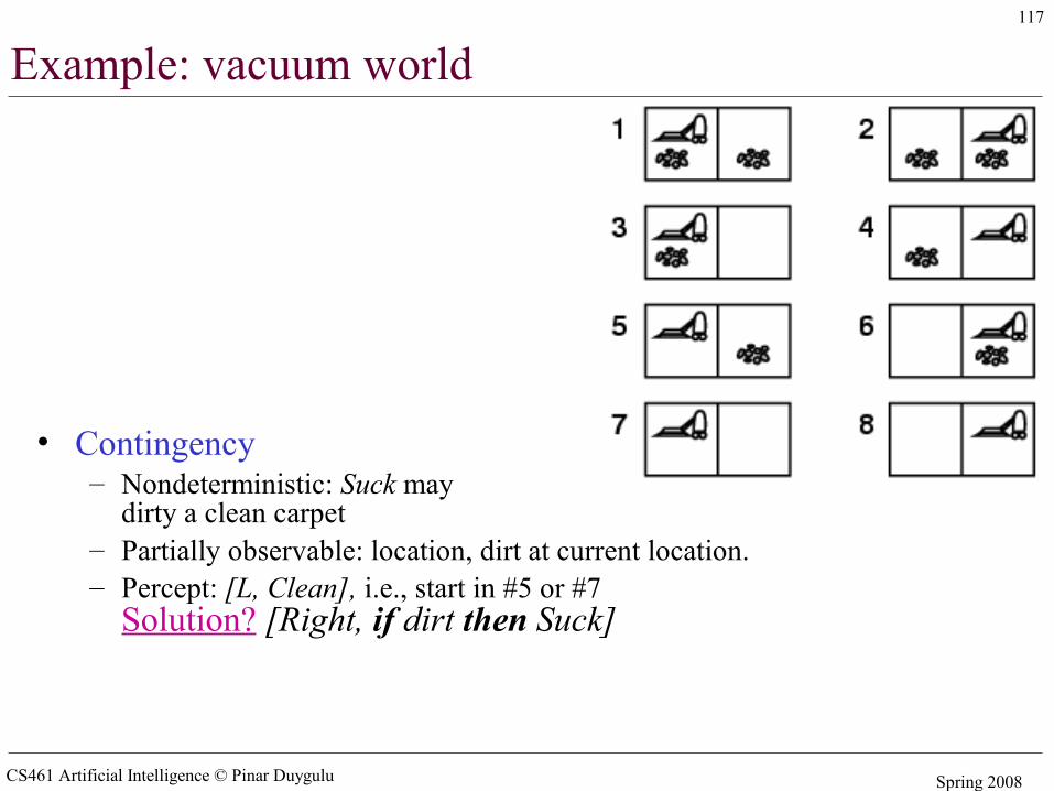
Example: vacuum world
• Contingency – Nondeterministic: Suck may
dirty a clean carpet– Partially observable: location, dirt at current location.– Percept: [L, Clean], i.e., start in #5 or #7
Solution? [Right, if dirt then Suck]
CS461 Artificial Intelligence © Pinar Duygulu Spring 2008
118
Summary
• Problem formulation usually requires abstracting away real-world details to define a state space that can feasibly be explored
• Variety of uninformed search strategies
• Iterative deepening search uses only linear space and not much more time than other uninformed algorithms