95

Chapter 3

Ruby Masers

Robert C. Clauss and James S. Shell

3.1 Introduction

Ruby masers are very low-noise pre-amplifiers used in the microwave

receiving systems of the Deep Space Instrumentation Facility (DSIF) and the

Deep Space Network (DSN) since 1960. Ruby masers are cryogenically cooled

to temperatures below 5 kelvin (K) to achieve extremely low noise levels, and

they are used near a focal point of large antennas for receiving signals from

spacecraft exploring the Solar System.

Microwave amplification by stimulated emission of radiation (maser) is

very different than the process in amplifying devices using a flow of electrons

in a crystal (such as transistors) or using a beam of electrons in a vacuum (such

as traveling wave tubes, klystrons, or triodes). The maser process may be

quantified in terms of photons. A photon at microwave frequencies might be

thought of as a particle or an amount of electromagnetic energy equal to hf

where h is Planck’s constant, 6.626 10–34

joule-seconds (J-s), and f is the

frequency in hertz (Hz). For example, at 8.42 gigahertz (GHz), a frequency

used for deep-space-to-Earth telecommunications, receiving one photon per

second provides an amount of power equal to 5.58 10–24

watts (W) or –202.5

decibels referenced to milliwatts (dBm). The power level of one photon per

second at 8.42 GHz is also equal to the noise power available from a 0.4041-K

source in a 1-Hz bandwidth. 0.4041 K is the hf/k quantum noise at 8.42 GHz,

where k is Boltzmann’s constant (1.38 10–23

joule/kelvin (J/K)). The ultimate

operating noise temperature lower limit of any linear receiving system is

accepted as the quantum noise.

96 Chapter 3

Ruby masers are the most sensitive and lowest noise microwave amplifiers

used in the field, yet they are rugged and are not susceptible to the microscopic

failures that sometimes occur in sub-micron junction devices. These

characteristics of ruby masers result from the stimulated emission process used

to amplify a signal. Stimulated emission is a photons-to-photons amplification

process. The paramagnetic ruby crystal contains chromium ions, and these ions

give the ruby a pink or red color. These ions each have three unpaired electrons.

The intrinsic spin angular momentum of each of these electrons gives them the

property of a magnetic moment. These three magnetic moments add together to

form a larger effective permanent magnetic dipole moment. This permanent

magnetic dipole moment associated with each chromium ion is referred to in

the following text as a “spin.” Spins in particular energy levels are excited by a

process called pumping, the application of microwave energy to the ruby.

Incoming signal photons stimulate the excited spins, which then drop from a

higher energy level to a lower energy level, thereby emitting photons in-phase

with, and in numbers proportional to, the stimulating signal photons. This

photons-to-photons amplification process enables linear low-noise

amplification while being quite immune to the generation of inter-modulation

products when strong signals interfere with the reception of weak signals. Ruby

masers can withstand input signal power levels of many watts without damage

and are not subject to burnout or damage by voltage transients.

Cavity masers using ruby were developed at the Jet Propulsion Laboratory

(JPL) at 960 megahertz (MHz) and at 2388 MHz. JPL’s first cavity maser

installed near the prime focal point on a 26-meter (m) diameter DSIF antenna at

a Goldstone, California Deep Space Station (DSS) is shown in Fig. 3-1. The

September 1960 occasion was JPL’s first liquid helium transfer into an

antenna-mounted maser at the DSS-11 “Pioneer” Site. The 960-MHz cavity

maser was cooled to 4.2 K by liquid helium in an open-cycle dewar. The maser

and the dewar were designed by Dr. Walter H. Higa and built by the group that

he supervised at JPL. This first experimental field installation and testing period

was followed by the installation of a 2388-MHz cavity maser in February 1961.

The 2388-MHz maser was used to receive and amplify microwave radar echoes

from the planet Venus [1]. Liquid helium was transferred on a daily basis at a

height of about 24 m above the ground, from the fiber-glass bucket of the

“cherry-picker” (High Ranger) seen in Fig. 3-1. Servicing the maser was

exciting work, especially when the wind speed reached 18 meters per second

(m/s) and buffeted the cherry-picker’s bucket.

Several single-cavity 960-MHz (L-band) masers were built, some using

open-cycle cooling and one cooled by a closed-cycle helium refrigerator [2]. A

dual-cavity 2388-MHz maser was developed and used at the Goldstone DSS-13

“Venus” Site to receive radar echoes from Venus and Mars [3]. Traveling-wave

maser (TWM) systems were developed for use at various S-band frequencies

Ruby Masers 97

Fig. 3-1. Liquid helium transfer. Including (a) manual transfer of

liquid helium at DSS-11 and (b) zoom-out view of cherry picker (high ranger) in use for liquid-helium transfer.

98 Chapter 3

between 2200 MHz and 2400 MHz, X-band frequencies between 7600 MHz

and 8900 MHz, and at Ku-band frequencies between 14.3 GHz and 16.3 GHz

[4]. K-band reflected-wave maser (RWM) systems were developed for radio

astronomy applications at frequencies between 19 GHz and 26.5 GHz. The

TWMs and RWMs all operated in closed-cycle refrigerators (CCRs) at

temperatures near 4.5 K. An RWM was developed to cover the 31.8-GHz to

32.3-GHz deep-space-to-Earth frequency allocation at Ka-band. A 33.7-GHz

two-cavity maser was developed and used at DSS-13 for the Ka-band link

experiment with the Mars Observer spacecraft [5].

Table 3-1 lists the ruby masers built for and used in the DSN. Twenty-

seven Block III S-band TWMs were implemented. 90 ruby masers were used in

the DSN since 1960. CCRs and other key parts were reused as they became

available, after replacement by later model masers. R&D masers were built and

used in the field, usually on the research antenna at DSS-13 and in the research

(radar) cone at DSS-14, to evaluate the long-term performance prior to

operational spacecraft tracking commitments. Occasionally R&D masers were

installed and used to support and enhance missions following spacecraft

problems that affected the communications link.

3.2 Ruby Properties

The pink ruby crystal used in maser amplifiers is about 99.95 percent

aluminum oxide (Al2O3) with approximately 0.05 percent chromium oxide

(Cr2O3). The paramagnetic Cr3+

ions occupy some of the sites normally

occupied by the Al3+

ions. Ruby used in the early cavity masers and TWMs was

grown by the flame-fusion process and usually contained multiple crystal

orientations and variations in the chromium concentration (doping gradients).

Inspection and selection of the ruby to find pieces of adequate size and quality

were needed. This inspection process was done in polarized light, using a cross-

polarized lens to view the flaws in the ruby. Superior quality ruby was

developed primarily for laser applications by the Union Carbide Corporation

using the Czochralski process. Czochralski ruby first became available for

maser applications in 1966.

Ruby is a hard, stable, rugged low-microwave-loss, and high-dielectric-

strength crystalline material that can be cut or ground to precise dimensions

with diamond tools. The dielectric constant is anisotropic, varying from 11.54

in the direction parallel to the axis of symmetry (c-axis) to 9.34 in the direction

perpendicular to the c-axis. The dielectric loss tangent is very low (< 0.0001)

and not measurable in ruby-filled cavities or in the slow-wave structures of

TWMs. Ruby survives repeated thermal cycling from ambient temperatures

above 300 K to cryogenic temperatures below 5 K. The thermal conductivity of

ruby is about 1 watt per centimeter-kelvin (W/cm-K) at 4 K and is adequate for

Ruby Masers 99

Table 3-1. DSN ruby maser history.

Time in Use

3

Frequency (GHz)

Maser Type Bath

Temp. (K)

Gain (dB)

Bandwidth (MHz)

Noise

Temp. (K)

Quantity3

1960–65 0.96 Cavity 4.2 20 0.75 17–301 5

1961 2.388 Cavity 4.2 20 2.5 25 1

1962–63 2.388 Dual cavity 4.2 34 2.5 18 1

1963–66 2.388 R&D TWM 4.5 40 12 8 1

1964–66 8.45 Multiple cavity 4.2 33 17 18 1

1964–71 2.295 Block I

S-band TWM

4.5 33 17 9–151 6

1965–71 2.27–2.30 Block II S-band TWM

4.5 35 17–30 9–151 8

1966–68 8.37–8.52 R&D TWM 4.5 30–45 17 18–231 1

1966–74 2.24–2.42 R&D TWM 4.5 27–50 16 4–61 3

1970–89 2.285 Block III

S-band TWM

4.5 45 40 4–61 27

1970–72 7.6–8.9 R&D TWM 4.5 30–42 17 7–131 1

1971–80 14.3–16.3 R&D TWM 4.5 30–48 17 8–131 1

1973–89 7.8–8.7 R&D TWM 4.5 45 17–20 7–111 1

1974–now 2.25–2.4 R&D TWM 4.5 30–50 15–30 2–41 1

1975–89 8.42 Block I

X-band TWM

4.5 45 40 5–101 12

1979–now 2.285 Block IV

S-band TWM

4.5 45 40 2 4

1980–now 8.45 Block II

X-band TWM

4.5 40 100 3–4.51 9

1981–95 18–25 RWM 4.5 30 100–300 12 3

1986–95 2.21–2.32 Block V S-band TWM

4.5 35–45 70 3–5 2

1992–now 8.475 R&D TWM 1.6 34 100 1.92 1

1992–94 33.3–34.0 Dual cavity 1.5 25 85 4–61,2

1

1 Range (varies across tuning range, from unit to unit, or due to measurement uncertainty)

2 At the feedhorn aperture

3 Quantities and time in use dates were obtained via personal communications with D. Hofhine of the Goldstone DSCC, and M. Loria of DSMS Operations.

100 Chapter 3

maser applications. For comparison, thermal conductivity of 50–50 lead-tin soft

solder is about 0.15 W/cm-K at 4 K, and the thermal conductivity of

electrolytic-tough-pitch copper is about 4 W/cm-K at 4 K.

3.3 Spin Resonance, the Applied Magnetic Field, Ruby Orientation, the Low-Temperature Requirement, and Excitation

The energy of the spins in ruby varies with the intensity and orientation of a

biasing magnetic field with respect to the c-axis of the ruby. Two different

orientations of ruby are used in JPL masers, depending upon the signal

frequency. The “90-degree” orientation used at L-band, S-band, X-band, and

Ku-band is discussed here. The “54.7-degree” orientation is discussed later in

the sections describing masers at X-band and higher frequencies. The direction

of the c-axis can be determined in polarized light.

The four ground-state microwave spin levels that occur are called

paramagnetic levels or Zeeman levels. The magnetic field strength and

orientation used for an S-band maser at a frequency near 2.4 GHz is given here,

for example. A magnetic field strength of 0.25 tesla (T) (2500 gauss (G)) is

applied to the ruby in a direction that is perpendicular to the c-axis. This is

called the 90-degree orientation. The energy spacings (hf) between the four

ground-state energy levels in ruby under these conditions were given in terms

of frequency (f). The spacing between these levels is: 1–2 = 2.398 GHz, 1–

3 = 12.887 GHz, and 1–4 = 24.444 GHz. Slightly more accurate values are

available today, but these values used during the development of masers at JPL

between 1959 and 1990 are sufficiently accurate.

The example above uses values from the Appendix, “Ruby energy levels

and transition-probability matrix elements,” in Microwave Solid-State Masers

[6]. Chang and Siegman published “Characteristics of ruby for maser

applications,” in 1958 [7]. Professor Siegman’s thorough history and

explanation of masers, together with his acknowledgment and descriptions of

the research work and publications of many in the maser field are not

duplicated here. His book contains a large volume of material about masers,

including much that was produced by many workers who shared their

knowledge generously. The extensive material published about maser theory

and techniques between 1956 and 1964 was most helpful, aiding in the timely

development of ruby masers at JPL for the Deep Space Network. Professor

Siegman’s book is recommended to those interested in the history of masers,

and for the detailed theory that leads to a better understanding of masers.

Spin resonance absorption in ruby-filled cavity or waveguide may be

observed with a microwave spectrometer as a function of frequency and an

applied magnetic field. Absorption of power occurs when signals are applied at

frequencies corresponding to the difference in frequency between energy levels.

Ruby Masers 101

The resonance absorption line-width of single crystal ruby with about

0.05-percent Cr3+

in a uniform magnetic field is about 55 MHz. This value, plus

or minus 10 percent, is independent of temperature and has been measured at

many different frequencies between 2 GHz and 40 GHz. The S-band example

above gives the three frequencies between the 1–2, 1–3, and 1–4 levels. Spin

resonance absorption also occurs at frequencies corresponding to the energy

differences between levels 2–3 (10.489 GHz), 2–4 (22.046 GHz), and 3–4

(11.557 GHz). The magnitude of the absorption depends upon the ratio of spins

in the various levels and is very weak at room temperature. At thermal

equilibrium, the ratio of spins in an upper state (Ni ) with respect to the lower

state (N j ) is an exponential function of energy difference and temperature.

The Boltzmann expression gives this ratio and the results show the need for

physically cooling the maser material to low cryogenic temperatures.

Ni

N j= e

h fijkT (3.3-1)

where h is Planck’s constant, fij is the frequency difference between levels i

and j in hertz, k is Boltzmann’s constant, and T is the thermodynamic (bath)

temperature in kelvins.

Consider the difference in the ratios of spins in levels 2 and 1 (N2 / N1) in

the S-band example above at various temperatures. When T = 300 K,

hf12 / kT = 3.8362 10–4

and the ratio is 0.99962. The two spin populations

are almost equal, and the absorption measured with a microwave spectrometer

is very weak. As the temperature is lowered from 300 K to 100 K, 20 K, 10 K,

4.5 K, 2.5 K and 1.5 K, the ratios (N2 / N1) decrease from 0.99962 to 0.99885,

0.99426, 0.98856, 0.97475, 0.95501, and 0.92615, respectively.

Whether large or small, when the ratio of spins in the upper level to the

lower level is less than 1, signal absorption occurs. Amplification by stimulated

emission depends on a population inversion where the ratio is greater than 1.

The low temperature advantage occurs in both the absorption case and the

emission case.

Inversion of the spin population between energy levels 1 and 2 requires the

use of an additional level or levels. The Boltzmann expression shows that, in

thermal equilibrium, the number of spins in each level decreases from the

lowest to the highest level. The example of the S-band maser at a temperature

of 4.5 K is used here. The ratio of spins in level 2 to level 1 is 0.97475. The

ratio of spins in level 3 to level 1 is 0.87159. The ratio of spins in level 4 to

level 1 is 0.77051. Application of a sufficiently strong pump signal at the

frequencies of either 12.887 GHz or 24.444 GHz will equalize the spin

102 Chapter 3

populations of levels 1 and 3, or 1 and 4. Either of these frequencies can be

used as the “pump” frequency to excite the spin system, to create a population

inversion.

The total number of spins in ruby with slightly more than 0.05 percent Cr3+

is about 2.5 1019

per cubic centimeter (cc). The S-band cavity maser used as

an example has a ruby volume exceeding 1 cc. The actual dimensions are not

important for this excitation example. The ratios of the spin densities (in spins

per cubic centimeter) in one level to another level are important. Consider x

number of spins in level 1 for the thermal equilibrium un-pumped case. The

spins in levels 1, 2, 3, and 4 are x, 0.97475 x, 0.87159 x, and 0.77051 x, for a

total spin population of 3.61685 x. The fraction of spins in each level are, level

1 = 0.27648, level 2 = 0.26950, level 3 = 0.24098, and level 4 = 0.21304. The

spin density values for each of the levels are level 1 = 6.9120 1018

, level 2 =

6.7375 1018

, level 3 = 6.0245 1018

, and level 4 = 5.3260 1018

. The level 2

spin density value is 1.745 1017

less than level 1. Equalizing the spins in

levels 1 and 4 reduces the spin density in level 1 from 6.9120 1018

to

6.1190 1018

[(6.9120 1018

+ 5.3260 1018

)/2]. The number of spins in level

2 and level 3 remain unchanged. The ratio of spins in level 2 to level 1 is now

1.1011, a ratio greater than one. The population inversion between levels 2 and

1, resulting from pumping between levels 1 and 4, provides 6.185 1017

more

spins per cubic centimeter (cc) in level 2 than in level 1.

Emission of the 6.185 1017

excess spins in level 2 in a 0.02-microsecond

( s) time period suggests that a pulse from a 1-cc ruby crystal at 2398 MHz

could reach 9.8 10–7

J (49 W for 2 10–8

seconds). This pulse is capable of

damaging a transistor amplifier following the maser, as demonstrated in the

laboratory during an unfortunate pulse-amplification experiment. A spin-

relaxation time of 50 ms for ruby at 4.2 K suggests this pulse amplification

process could be repeated at a rate of 20 times per second, resulting with an

equivalent continuous power level of about 20 microwatts (–17 dBm). This is

about twice the maximum emission level of a –20-dBm signal observed to be

available from an S-band TWM. Such a TWM, with low-level signal net gain

of 45 dB shows about 1 dB of gain compression when the input signal reaches

–84 dBm (the maser output signal is –40 dBm). The maser gain decreases

gradually as the input signal strength is increased until the input reaches

–20 dBm. At this point, the maser is a unity-gain amplifier. Increasing the input

signal above –20 dBm causes the TWM to become a passive attenuator.

Pumping the S-band maser between levels 1 and 4 in the example above

appears to give much better maser performance than would be achieved by

pumping between levels 1 and 3. Measurements show that this is not the case.

This simple example does not include other considerations that affect the

performance of masers. Various parameters, including the spin-lattice

relaxation time, inversion ratios, transition probabilities, and the filling factor

must be considered.

Ruby Masers 103

3.4 Spin-Lattice Relaxation Time, Inversion Ratios, Transition Probabilities, the Filling Factor, and Magnetic Q

It is expedient to use the spin-lattice relaxation times measured and

published by others. For ruby, in the microwave region at a temperature of

4.2 K, these times are of the order of 0.050 seconds. Below 5 K, these times are

roughly inversely proportional to temperature [6, p. 225]. It seems reasonable to

expect the spin relaxation times for the various levels to be roughly equal.

Optimum spin relaxation times provide higher inversion ratios than equal spin

relaxation times. Inversion ratios also vary in accordance with the pumping

scheme used. Siegman, [6, p. 292 and 293] mentions four multiple pumped

schemes and gives inversion ratio equations for the single-pumping three-level

scheme and the multiple-pumping push-pull scheme. The signal frequency ( fs )

and the pump frequency ( fp ) in the three-level scheme used at S-band results

in inversion ratios of ( fp / fs ) – 1 for the case of optimum spin-relaxation

times and ( fp / 2 fs ) – 1 for the case of equal spin relaxation times.

The actual inversion ratio is determined by measuring the signal frequency

amplification (the electronic gain in decibels) in the pumped case and dividing

it by the signal frequency spin system absorption (in decibels) in the un-

pumped case. Spin system absorption and inversion ratios were measured

experimentally for many ruby orientations at many different frequencies and for

other potential maser materials as well. The measurements at JPL used either a

small dielectric resonator in waveguide, in the reflection mode, or the slow-

wave structure of a TWM operating in the transmission mode. The use of a

dielectric resonator in the reflection mode gives reliable results when the

absorption values are a few decibels and amplification values are modest,

between a few decibels and 10 dB. Regenerative gain can give gain values

higher than those caused by the actual inversion ratio and must be avoided

during the inversion ratio measurements.

Our most accurate inversion ratio measurements for S-band used a TWM at

2295 MHz. The pump frequencies used were 12.710 GHz (1–3 transition) and

24.086 GHz (1–4 transition). These calculated inversion ratios are shown in

Table 3-2, along with the measured inversion ratios.

The absolute accuracy of the inversion ratio measurement could not resolve

the ratio to better than ±0.1, but the difference between the two measurements

observed by alternately turning the pump sources on and off was more precise,

and it clearly showed the slight advantage for the higher frequency pump.

Pump power was adequate for complete maser saturation in both cases.

The results of these inversion ratio tests at 2295 MHz suggest one of three

possibilities: (1) The measured inversion ratio of 4.5 is close to the calculated

104 Chapter 3

value of 4.54 for the 12.710-GHz pump case with optimum spin relaxation

times; (2) The measured ratio of 4.6 is less than half of the value of 9.5

calculated for the 24.086-GHz pump case with optimum spin relaxation times,

but is not far above the calculated value of 4.25 for the 24.086 pump case with

equal spin relaxation times. One might assume that the spin relaxation time

from level 3 to level 2 is much shorter than the spin relaxation time from level 2

to level 1, the optimum case. One might also assume that the spin relaxation

time from level 4 to level 2 is slightly shorter than the spin relaxation time from

level 2 to level 1. Both assumptions could explain the results; (3) There might

also be a third explanation for the apparent almost ideal inversion ratio obtained

with the 12.710-GHz pump, one that includes nearly equal spin relaxation

times. The spacing between level 3 and level 4 is 11.376 GHz, the difference in

frequency between the 24.086 GHz pump frequency and the 12.710 frequency.

This 3–4 transition has an extremely strong transition probability. The action of

the 12.710-GHz pump, that pumps spins from level 1 up to level 3, may also

elevate spins from level 3 to level 4, achieving an effect similar to pumping

from level 1 to level 4 directly with 24.086 GHz. This process, called push-

push pumping, will receive more attention in the X-band maser section of this

chapter.

Transition probabilities for the various ruby orientations and for various

magnetic field strengths are given in the appendix to Professor Siegman’s book

[6] that was mentioned earlier. Transition probabilities are directional, having a

maximum-probability direction and a zero-probability direction called the null

direction. In the case of the 90-degree (deg) orientation where the applied

magnetic field is perpendicular to the c-axis, we find the null direction for the

signal frequency transition is in the direction of the applied magnetic field. Any

microwave magnetic field components in this direction will not interact with

the spin system. The c-axis direction is the direction of maximum signal

transition probability for the 90-deg orientation in ruby and the radio frequency

(RF) magnetic field components in this direction will have the maximum

interaction with the spin system at frequencies below 15 GHz. A third direction,

perpendicular to the plane determined by the c-axis direction and the applied

magnetic field direction, has a transition probability less than the maximum

transition probability at frequencies below 15 GHz, being about one-tenth the

maximum transition probability at 2295 MHz.

Table 3-2. Inversion ratios for a 2295-MHz TWM.

Calculated Inversion Ratios for Pump

Frequency (GHz)

Equal Spin Relaxation Times

Optimum Spin Relaxation Times

Measured

Inversion Ratios

12.710 1.77 4.54 4.5

24.086 4.25 9.5 4.6

Ruby Masers 105

A ruby-filled coaxial cavity, similar to the one used at the 2388-MHz maser

for the Venus radar in 1961, is used to give a visual example of the RF

magnetic field interaction with the ruby spin system. Figure 3-2 shows the

cavity in which the center conductor is shorted at the bottom and open

wavelength from the bottom. The ruby cylinder has a 1.9-cm outside diameter

with a 0.636-cm hole through the center, and it is approximately 1 cm in length.

The outside diameter of the ruby fits tightly into a copper outer conductor, and

the center conductor of the -wavelength resonator is a close fit in the

0.636-cm hole. The center conductor extends slightly beyond the ruby, and this

length is adjusted to obtain resonance at the signal frequency. The signal is

coupled through the capacitor formed by a sapphire sphere located between the

center conductor of the -wavelength cavity and the open-ended center

conductor of the coaxial transmission line shown in part above the maser. The

orientation of the sapphire sphere affects the capacitive coupling to the cavity

Direction of AppliedMagnetic Field

Ruby c-AxisDirection

Coaxial Line forSignal Input/Output

Sapphire Sphere

Ruby in 1/4Wavelength CoaxialResonator

Ruby c-Axis

Direction30-degAngle

Top View

Side View

Fig. 3-2. Ruby-filled 2388-MHz coaxial cavity maser. (The ruby c-axis is also the z-axis of maximum transition probability.)

30 deg outof Page

x

zy

106 Chapter 3

and the resulting cavity resonant frequency; this is caused by the anisotropy of

the sapphire’s dielectric constant. Figure 3-3 shows a cross-sectional view of

the coaxial cavity maser and dewar system.

The ruby cavity is located inside of a liquid helium dewar for cooling to

4.2 K. The ruby c-axis direction in the cavity forms a 60-deg angle with the

direction of the center conductor as shown in Fig. 3-2. The applied magnetic

field of about 0.25 T comes from a magnet located at room temperature, outside

the dewar. The coaxial transmission line and ruby-filled cavity is rotated until

the ruby c-axis direction is perpendicular to the direction of the magnetic field.

The directional transition probabilities in “ruby energy levels and

transition-probability matrix elements” [6] are given in terms of alpha, beta,

and gamma, corresponding to the x, y, and z directions in Fig. 3-2. In this case

the x-direction, being the same direction as the applied magnetic field direction,

is the null-direction. The c-axis direction is the z-direction of maximum

transition probability and is the direction of greatest importance. The projection

of the z-direction into the plane of the circular RF magnetic field determines the

resultant efficiency or filling factor of about 0.43 for the signal frequency

interaction with the spin system. The projection of the y-direction into the plane

of the circular RF magnetic field is such that the interaction between the spin

system and the RF magnetic field in that part of the cavity is very low, having

little affect on amplification. The transition probability in the y-direction is

about 1/10 of the transition probability in the z direction. If the c-axis of the

ruby had been perpendicular to the direction of the center conductor, in the

plane of the signal frequency RF magnetic field, the filling factor would have

been near the maximum value of 0.5. The combination of the circular RF

magnetic field pattern and the linear c-axis direction results in a 0.5 maximum

filling factor when the entire cavity is filled with ruby. The important

considerations in determining the filling factor are the placement of the active

material in the regions where the RF magnetic field is strong, and a parallel

alignment of the RF magnetic field direction with respect to the direction of

maximum transition probability.

The filling factor, inversion ratio, and transition probability values all affect

the maser’s amplifying ability. These, combined with the physical temperature,

the maser material’s spin density, the number of energy levels, the frequency,

and the maser material 55-MHz line-width, determine the magnetic Q value

(Qm ) . Qm is used to calculate the gain of a maser, be it a cavity maser, a

traveling-wave maser, or a reflected wave maser. A simplified approximation

for the Qm of ruby with 0.053-percent Cr3+

(a spin density of 2.5 1019

spins/cm3) at frequencies below 10 GHz and temperatures above 4 K is

Qm(141) T

fI 2 (3.4-1)

Ruby Masers 107

Fig. 3-3. Cross-section of a coaxialcavity maser and dewar system.

Circulator

Pump Power Input

CoaxialTransmission Line

LiquidNitrogenTank

LiquidHeliumTank

Ruby Crystal

Vernier Coil

N S

Permanent Magnet

Liquid HeliumFill Tube

LiquidNitrogenFill Tube

OutputInput

108 Chapter 3

where

T = the thermodynamic temperature, K

f = the frequency, GHz

I = the inversion ratio 2 = the maximum value of the transition probability matrix

elements, and

= the filling factor

A Qm of 71.6 is calculated using I = 4.3, 2= 1.6 , and = 0.5 for the

2.398-GHz cavity maser at 0.25 T (2500 G) and at 4.2 K. Siegman indicates

[6, p. 255] that the approximation hf / kT << 1 holds for this estimate of

magnetic Q.

The use of the actual spin density difference ( N ) between the two levels

adjacent to the signal transition results in a magnetic Q calculation that is not

dependent upon hf / kT << 1 .

Qm =4.22 1019

( N )I 2 (3.4-2)

The thermal equilibrium (un-pumped) spin density values for the 2.398-GHz

cavity maser example at 4.2 K are level 1 = 6.95925 1018

, level 2 = 6.77125

1018

, level 3 = 6.00625 1018

, level 4 = 5.26325 1018

. N = 1.88 1017

.

Qm =4.22 1019

1.88 1017 (4.3) (1.6) (0.5)= 65.2 (3.4-3)

The Qm values of 71.6 for the approximation and 65.2 for the more exact

calculation of the S-band example are within 10 percent of each other,

suggesting that the low-frequency high-temperature approximation

( hf / kT << 1) is useful in some cases.

An example of a maser at a higher frequency and a lower temperature uses

the 33.7-GHz maser at 1.5 K. Here I = 2, 2= 1 , and = 0.5 . Using the

approximation from Eq. (3.4-1) for this case, we calculate a Qm of 6.26. The

energy level distribution for the 33.7-GHz maser is calculated using the

equation for the Boltzmann distribution. The frequencies corresponding to these

levels are 1–2 = 35.92 GHz, 1–3 = 69.62 GHz, and 1–4 = 105.54 GHz. The

signal frequency transition is the 2–3 transition at 33.70 GHz. The thermal

equilibrium (un-pumped) spin density values for the 33.70-GHz cavity maser

at 1.5 K are: level 1 = 1.7137 1019

, level 2 = 5.4303 1018

, level

Ruby Masers 109

3 = 1.8473 1018

, and level 4 = 5.8850 1017

. N , the difference between

level 2 and level 3, is 3.5830 1018

. The Qm given by Eq. 3.4-2 is 11.77, a

factor of 1.88 higher than the Eq. 3.4-1 approximation. Use of the

approximation is not acceptable for the higher frequency and lower temperature

Qm calculations.

The gain of a maser depends upon Qm and upon the interaction time

between the RF magnetic field and the spin system. The interaction time in a

cavity maser is dependent on Q1 , the loaded Q of the cavity. The cavity maser

electronic gain equation in decibels is

GedB

= 10 logQ1 + Qm( )

Q1 Qm( )

2

(3.4-4)

The interaction time in a TWM is dependent upon the TWM’s electrical length,

the slowing factor (S) multiplied by the physical length in wavelengths (N). The

TWM electronic gain equation in decibels is

GedB

=(27.3) S N

Qm (3.4-5)

These equations are simplified but accurate forms, derived from those found in

[6, pp. 268 and 309]. Ruby masers developed at JPL from 1959 through 1992

were based on the material described above. These designs were analyzed by

using performance measurement data of the amplifying structures.

Future waveguide-cavity maser designs and TWMs using waveguide

resonators as slow-wave structures can be analyzed using computer programs.

Various 32-GHz ruby maser designs have been created and analyzed using a

combination of commercial design software and a specialized JPL-developed

program based on a waveguide mode-matching algorithm. The new analysis of

maser designs will be described in a later part of this chapter.

3.5 Ruby Maser Noise Temperatures

A distinct advantage of the ruby maser is its low effective input noise

temperature (Tampl ) . It is also an advantage that the maser noise temperature

can be calculated accurately and reliably from the maser gain-and-loss

characteristics. The maser net gain, the structure loss, the ruby “pump off” spin-

system loss, and the thermodynamic or bath temperature of the maser (Tb ) are

needed for the noise temperature calculation.

110 Chapter 3

The equation used for an accurate calculation of a ruby maser’s equivalent

input noise does not require that hf / kT be much less than one. It is accurate at

all frequencies and temperatures, and it includes the quantum noise

contribution. The maser’s noise temperature is predicted with calculations

broken into two parts. The first part accounts for the noise temperature of the

ruby spin system. The second part accounts for noise contributed by the

dissipative losses in the slow-wave structure of a TWM, RWM, or in the

resonators of a cavity maser. Noise contributions from dissipative losses in

components preceding the maser must be accounted for separately.

Siegman has described and discussed noise, in masers and in general

[6, p. 398], and Siegman derives the noise power from a maser to be

Pn(ampl) = (G 1) m

m 0

Pn ( m , Tm ) +o

m oPn ( o,To ) (3.5-1)

where Siegman’s symbols, m and o , are the electronic gain and loss

coefficients per unit length, ( m o ) is the net gain coefficient per unit

length, and Ts , the spin temperature, equals Tm . This expression is valid for a

traveling-wave maser (TWM), a reflected-wave maser (RWM), and the

reflection-type cavity maser.

Numerically, the gain and loss coefficient ratios can be replaced by ratios

of the maser’s electronic gain Ge(dB) , net gain G(dB)

, and loss Lo(dB) in

decibels. Therefore, m / ( m o ) equals Ge(dB) / G(dB) and o / ( m o )

equals Lo(dB) / G(dB) , where the electronic gain is provided by the inverted ruby

spin system and the loss is the signal attenuation due to dissipation. The

dissipation is caused by the resistance of the copper or other metals used in the

structure, by dielectric material loss, and by ferrite or garnet isolator forward

loss in the case of a TWM. This loss term, Lo(dB) , does not include the spin-

system signal absorption that occurs when the maser is not pumped. The net

gain in decibels is the electronic gain in decibels minus the loss in decibels.

Using the measured gain and loss values in decibels, and replacing Pn (T )

with the Planck radiation law

Pn (T ) =h fB

e

h f

kT 1

(3.5-2)

The equation for the noise power from the maser becomes

Ruby Masers 111

Pn(ampl) = (G 1)Ge

dB

GdB

h fB

1 e

h f

kTm

+Lo

dB

GdB

h fB

e

h f

kTo 1

(3.5-3)

and the noise temperature of the maser becomes

Tampl =G 1

G

h f

k

GedB

GdB

1

1 e

h f

kTm

+Lo

dB

GdB

1

e

h f

kTo 1

(3.5-4)

The spin temperature is determined by the ratio of the spin population densities

in the two levels associated with the signal transition.

r =ni

n j= e

h f

kTs = e

h f

kTm (3.5-5)

The ratio r is substituted in Eq. (3.5-4), resulting in the simplified form

Tampl =G 1

G

h f

k

GedB

GdB

r

r 1+

LodB

GdB

1

e

h f

kTo 1

(3.5-6)

“Pump saturation” is a requirement meaning the pump power is sufficient

to equalize the spins in the energy levels spaced properly for pump excitation.

Verification of this pump-saturated condition is determined by increasing the

pump power until no further increase in maser gain is observed. The pump-

saturated inverted spin population density ratio between levels i and j, denoted

by r = ni / n j , is determined by the difference between the thermal equilibrium

level spin densities and the inversion ratio I.

I =ni n j

N j Ni=

GedB

LrdB

(3.5-7)

Ni is the spin population of level i when the spin system is in thermal

equilibrium, and ni is the spin population in level i when the ruby spin system

is saturated with pump power. The inversion ratio is numerically equal to the

ratio of the electronic gain in decibels, with the microwave pump source on, to

the ruby absorption in decibels, Lr(dB) , with the microwave pump source off.

112 Chapter 3

Depending on the pumping scheme, the expression for r is different. For the

three-level system used at S-band, at the 90-deg orientation, the signal

transition is between levels 1 and 2, and the pump transition is between levels 1

and 3. The 4th

level is not involved, and the number of spins in it is unaffected

by the pumping. Pumping equalizes the number of spins in levels 1 and 3, and

two equations for the populations in each level are:

n2 n1 = I (N1 N2 ) (3.5-8)

and

n2 + 2n1 = N (3.5-9)

where N is the total number of spins in levels 1, 2, and 3; and

N = N1 + N2 + N3 = n1 + n2 + n3

Multiplying Eq. (3.5-8) by 2 and adding the resulting product to Eq. (3.5-9)

results in

3n2 = N + 2I (N1 – N2 ) (3.5-10)

Subtracting Eq. (3.5-8) from Eq. (3.5-9) results in

3n1 = N – I (N1 – N2 ) (3.5-11)

Dividing Eq. (3.5-10) by Eq. (3.5-11) results in

rs =1+ 2I (N1 N2 )

1 I (N1 N2 ) (3.5-12)

where Ni = Ni / N

A four-level push-push pumping scheme is used at X-band and Ku-band,

and it may also be used at S-band. The signal transition is between levels 1 and

2, and the pump transitions are between levels 1 and 3 and also between levels

3 and 4. Calculating the spin densities in the four levels, using the knowledge

that levels 1, 3, and 4 are equalized by pumping, and using the measured

inversion ratio I, the ratio of spins in level 2 divided by level 1 is

rx =1+ 3I (N1 N2 )

1 I (N1 N2 ) (3.5-13)

where Ni = Ni / N and N is the total number of spins in levels 1, 2, 3, and 4.

Ruby Masers 113

A four-level push-pull pumping scheme is used with JPL masers at K-band

and Ka-band. The signal transition is between levels 2 and 3, and the pump

transitions are between levels 1 and 3 and also between levels 2 and 4. The

54.7-deg ruby orientation produces symmetrical energy levels, so that the 1–3

transition is equal to the 2–4 transition. Calculating the spin densities in the four

levels is similar to the processes above. Using the knowledge that the spin

density in level 1 equals the spin density in level 3, and that the spin density in

level 2 equals the spin density in level 4, and the using the measured inversion

ratio I, the ratio of spins in level 3 divided by level 2 is

rk =1+ 2I (N1 N2 )

1 2I (N1 N2 ) (3.5-14)

where Ni = Ni / N

In contrast with the noise temperature calculations described above, a very

simple equation can be used to calculate the approximate noise temperature of a

maser (Tmaprx ) when hf / kT is much less than one and when the maser gain is

very high [5].

(Tmaprx ) = TbLt

(dB)

G(dB) (3.5-15)

where Lt(dB)

is the forward loss through the maser structure in decibels with the

pump turned off. This loss includes all dissipative losses, such as resistive

losses in copper, forward isolator losses, dielectric losses and the ruby (spin-

system) signal absorption. G(dB) is the net gain of the maser in decibels. Tb is

the thermodynamic temperature or bath temperature of the ruby. A comparison

of the results is shown in Table 3-3.

Table 3-3. Tmaprx values compared with accurate Tampl calculation results.

Parameter Value

Frequency (GHz) 2.295 8.430 33.7

Bath temperature (Tb) (K) 4.5 1.6 4.5 1.5

Tmaprx (K) 1.61 0.89 2.15 0.83

Tampl (K) 1.64 1.02 2.23 2.33

Difference (K) –0.03 –0.13 –0.08 –1.50

114 Chapter 3

Table 3-3 shows reasonable Tmaprx values for S-band masers at 2295 MHz

and X-band masers at 8430 MHz operating at a bath temperature of 4.5 K. The

value of hf / kT is 0.0245 at 2295 MHz and 4.5 K, and 0.0899 at 8430 MHz

and 4.5 K. At 8430 MHz and a bath temperature of 1.6 K, the value of hf / kT

is 0.2529, and the error of the Tmaprx calculation is about <15 percent. It seems

best to use the more accurate noise temperature calculation when hf / kT is

greater than 0.1. Maser performance values used to calculate the maser noise

temperatures are shown in Table 3-4.

Variations of maser noise temperature caused by changes in loss, inversion

ratio, and bath temperature are quantified to help determine the accuracy of the

maser noise temperature. For example, the TWM at 2295 MHz in Table 3-3 is

based on a slow-wave structure forward loss of 5 dB. An increase of 1 dB in the

structure forward loss value causes a noise temperature increase of 0.12 K. An

inversion ratio reduction from 4.5 to 4.0 causes a noise temperature increase of

0.14 K. An increase in the bath temperature from 4.5 K to 4.7 K causes a gain

reduction of 2 dB and a noise temperature increase of 0.10 K. Maser

performance characteristics at 8430 MHz and 33.7 GHz can be measured to

accuracies that are little different than those at 2295 MHz. For example, at

33.7 GHz and a bath temperature of 1.5 K, a bath temperature increase to 1.7 K

increases the maser noise temperature by less than 0.1 K. Similar percentage

changes of loss and inversion ratio cause maser noise temperature changes of

less than 0.1 K. Based on these sensitivity values and our ability to measure

maser performance gain and loss characteristics to a fraction of a dB, and the

bath temperature to better than 0.1 K, all calculated maser noise temperatures

are expected to be accurate to within ± 0.1 K.

These Tampl maser noise temperature values are for the input to the ruby

maser at the bath temperature. In the case of a cavity maser, the noise

contribution of the circulator preceding the cavity amplifier must be added. In

all cases, any loss preceding the maser adds noise to the maser and the

Table 3-4. Maser performance values for noise temperature calculations.

Parameter Value

Signal frequency (GHz) 2.295 8.430 33.7

Bath temperature (Tb) (K) 4.5 4.5 1.6 1.5

Net gain (dB) 45.0 45.0 34.0 27.0

Electronic gain (dB) 50.0 49.0 39.0 28.0

Structure loss (dB) 5.0 4.0 5.0 1.0

Inversion ratio 4.5 2.8 2.8 2.0

Ruby Masers 115

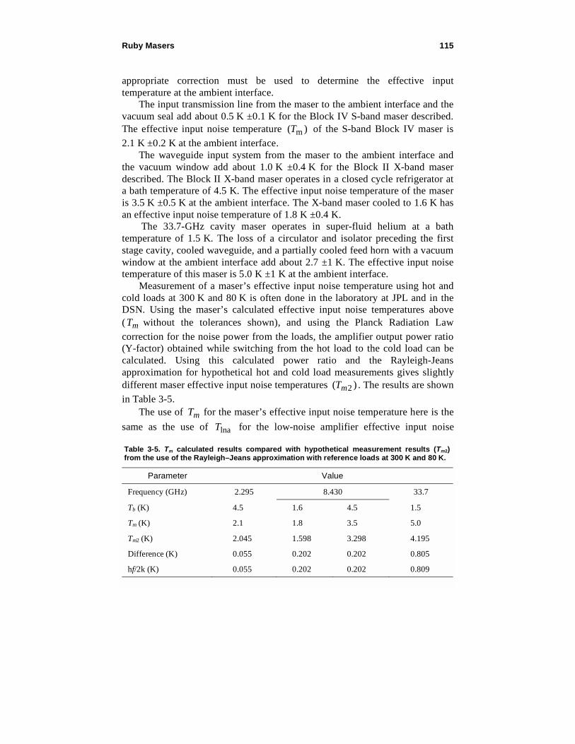
appropriate correction must be used to determine the effective input

temperature at the ambient interface.

The input transmission line from the maser to the ambient interface and the

vacuum seal add about 0.5 K ±0.1 K for the Block IV S-band maser described.

The effective input noise temperature (Tm ) of the S-band Block IV maser is

2.1 K ±0.2 K at the ambient interface.

The waveguide input system from the maser to the ambient interface and

the vacuum window add about 1.0 K ±0.4 K for the Block II X-band maser

described. The Block II X-band maser operates in a closed cycle refrigerator at

a bath temperature of 4.5 K. The effective input noise temperature of the maser

is 3.5 K ±0.5 K at the ambient interface. The X-band maser cooled to 1.6 K has

an effective input noise temperature of 1.8 K ±0.4 K.

The 33.7-GHz cavity maser operates in super-fluid helium at a bath

temperature of 1.5 K. The loss of a circulator and isolator preceding the first

stage cavity, cooled waveguide, and a partially cooled feed horn with a vacuum

window at the ambient interface add about 2.7 ±1 K. The effective input noise

temperature of this maser is 5.0 K ±1 K at the ambient interface.

Measurement of a maser’s effective input noise temperature using hot and

cold loads at 300 K and 80 K is often done in the laboratory at JPL and in the

DSN. Using the maser’s calculated effective input noise temperatures above

(Tm without the tolerances shown), and using the Planck Radiation Law

correction for the noise power from the loads, the amplifier output power ratio

(Y-factor) obtained while switching from the hot load to the cold load can be

calculated. Using this calculated power ratio and the Rayleigh-Jeans

approximation for hypothetical hot and cold load measurements gives slightly

different maser effective input noise temperatures (Tm2 ) . The results are shown

in Table 3-5.

The use of Tm for the maser’s effective input noise temperature here is the

same as the use of Tlna for the low-noise amplifier effective input noise

Table 3-5. Tm calculated results compared with hypothetical measurement results (Tm2) from the use of the Rayleigh–Jeans approximation with reference loads at 300 K and 80 K.

Parameter Value

Frequency (GHz) 2.295 8.430 33.7

Tb (K) 4.5 1.6 4.5 1.5

Tm (K) 2.1 1.8 3.5 5.0

Tm2 (K) 2.045 1.598 3.298 4.195

Difference (K) 0.055 0.202 0.202 0.805

hf/2k (K) 0.055 0.202 0.202 0.809

116 Chapter 3

temperature in other chapters of this book. Table 3-5 shows the differences in

the effective input noise temperature of masers caused by the differences in the

reference load noise powers that result from the use of the Rayleigh–Jeans

approximation. These differences are very close to one-half of the quantum

noise ( hf / 2k ) for the cases analyzed. A more detailed explanation of this

result was published previously [8,9]. System operating noise temperature

measurements in the DSN currently use the Rayleigh-Jeans approximation.

3.6 Ruby Masers as Noise Temperature Standards

The DSN ruby masers used as pre-amplifiers to achieve the lowest practical

receiving system noise temperatures are also used as noise standards. The

maser’s effective input noise temperature (Tm ) determines the receiver’s

effective input noise temperature (Te ) and enables the accurate measurement of

the total receiving system’s operating noise temperature (Top ) . Top is the sum

of Te and the antenna output temperature (Ti ) . Top here is defined at the

ambient input terminal of the maser, which is the reference 2 location defined

in Chapter 2. In this case, Ti includes the sky brightness temperature, antenna

pickup from ambient surroundings, noise contributed by reflector losses, and

noise contributed by feed system loss when the feed system components are at

ambient temperature. Use of masers as noise standards eliminates the need for

cryogenically cooled reference terminations in DSN receiving systems.

DSN receiving systems use a waveguide switch and a room temperature

load, or an ambient temperature absorber (aperture load) that can be positioned

in front of the antenna feed-horn. The aperture load is used to terminate the

receiver with a resistive source of known (ambient) temperature. The power

ratio measured when the receiver’s input is switched from the ambient load to

the antenna is used to determine Top .

DSN ruby masers at 2295 MHz, 8430 MHz, and 33.70 GHz achieved

effective input noise temperatures of 2.1 K ±0.2 K, 1.8 K ±0.5 K, 3.5 K ±0.5 K,

and 5.0 K ±1.0 K respectively, as explained in the previous paragraphs. The

measured values agreed with the calculated maser effective input noise

temperatures (Tm ) at the maser’s ambient interface.

The receiver’s effective input noise temperature (Te ) is the sum of the

maser noise temperature (Tm ) and the follow-up receiver noise contribution.

High DSN maser gain (typically 45 dB) reduces the follow-up receiver noise

contribution to a value that can be measured in two different ways. The follow-

up receiver noise temperature can be measured using hot and cold loads. The

measured receiver noise temperature is then divided by the maser gain to

determine the receiver’s contribution to Top . For example, when the noise

Ruby Masers 117

temperature of the receiver following the maser is 1000 K and the maser gain is

45 dB (31,623), the follow-up receiver contribution (Tf ) to Ta is

1000/31623 = 0.0316 K.

Turning the maser pump source off and on and measuring the resulting

receiver power ratio is another method to determine (Tf ) . This technique,

suggested by Dr. R. W. DeGrasse in 19621, has been used since in the DSN. In

this case, the maser with a 2.1-K noise temperature is connected to an ambient

termination near 290 K and receiver output power ratio, Ypump , is measured

while turning the maser pump source off and on.

Without the knowledge of the follow-up receiver noise temperature, as used

in the first example,

Tamb + Ta + Tf

T f= Ypump (3.6-1)

and

Tf =Tamb + Ta

Ypump 1 (3.6-2)

Substituting the known values for the ambient load (290 K for example) and the

maser we find

Tf =290 K+ 2.1 K

Ypump 1 (3.6-3)

A large value of Ypump is observed when the maser gain is 45 dB. The

1000-K follow-up receiver temperature mentioned above results in a 39.66-dB

Ypump measurement. A 10,000-K follow-up receiver temperature would result

in a 29.66-dB Ypump measurement, indicating a 0.316-K follow-up receiver

contribution. A phone call to a receiver repair person would be in order

following such a receiver noise temperature measurement.

A small error in Tf occurs when using the pump on–off method if the

maser’s pump-off loss is low, and a low-noise follow-up amplifier is used with

a maser having modest gain. This error occurs when the noise from the ambient

load, attenuated by the maser’s pump-off loss, is a significant fraction of the

follow-up amplifier noise temperature. Performance values for the 33.68-GHz

1 Personal communication from Dr. R. W. DeGrasse to R. Clauss in 1962.

118 Chapter 3

dual cavity maser are used here for example. The pump-off loss of 17 dB

(14 dB ruby absorption and 3 dB microwave component loss) allows 6 K from

a 300-K ambient load to reach the follow-up amplifier. The cooled high

electron mobility transistor (HEMT) follow-up amplifier had an effective input

noise temperature of 40 K. At 25-dB maser gain, the follow-up noise

temperature was 0.1265 K. Using the pump on/off technique results in a follow-

up calculation of 0.1455 K which is high by 0.019 K.

When the maser in the examples above is switched from the ambient load

to the antenna, the measured power ratio (Yamb-ant ) is used to determine Top .

Top =Tamb + Tm + Tf

Yamb-ant (3.6-4)

For example, when (Yamb-ant is equal to 25.12 (14.00 dB), Top = 11.624 K.

This S-band example is used because it is similar to the results achieved with

the DSN’s S-band receiving system on the 70-m antenna in Australia (DSS-43)

used to support the Galileo Mission during recent years. This S-band maser was

originally developed to support the Mariner-10 Mercury encounters in 1974

[10]. Top measurements at X-band and Ka-band in the DSN use the same

techniques described above.

The accuracy of the ruby maser’s effective input noise temperature affects

the accuracy of the system operating noise temperature measurement when the

maser is used as a noise standard. The S-band example can be used to show that

a 0.2-K error in maser noise temperature results in a 0.008-K error in Top . The

error is very small because the (Yamb-ant ) ratio is large. Top values measured

with the antenna at the zenith, looking through one atmosphere in clear dry

weather, range from the S-band low value to typical values of near 20 K at

X-band and 30 K for the 33.70-GHz maser system used at DSS-13. The Top

error caused by a Tm error is proportional to Top . For example, a 1-K error in

Tm causes a 0.07-K error in Top when Top is 21 K, a 0.1-K error when Top is

30 K, and a 0.2-K error when Top is 60 K.

Directional couplers are used in a DSN receiving system to inject signals

before and after the maser preamplifier to measure the maser gain. The

directional coupler between the antenna feed and the maser is also used to inject

a small amount of noise from a noise source (gas tube or noise diode). An

advantage of using a small amount of injected noise, that can be turned on and

off, is to monitor Top without disconnecting the receiver from the antenna. The

injected noise pulse becomes a secondary measurement standard; the noise

Ruby Masers 119

pulse excess temperature is determined by comparison with the total system

noise power when the maser is connected to the ambient load.

Another important advantage occurs when injecting a signal, or a small

amount of noise, while the receiver is alternately connected to the antenna, and

the ambient temperature termination. This technique enables the detection of

receiver gain changes that might occur when the receiver is switched from the

antenna to the ambient termination. Measurement of any receiver gain change

that occurs when switching between the antenna and the ambient termination

can be used to correct the error that results from the receiver gain change.

Loads or terminations at different temperatures, often at cryogenic and

ambient temperatures, can be used to measure receiver noise temperatures. The

effective noise temperature of loads at temperatures other than ambient depend

upon accurate knowledge of the dissipative surface of the load, and the

temperature gradient and loss of the transmission line used to thermally isolate

the load from the switch between the receiver and the load. Errors in the

effective temperature of cryogenically cooled loads can be caused by moisture

condensing upon portions of the interconnecting transmission lines and

windows (or gas barriers) required to separate the cryogenic system from the

ambient environment.

The maser noise temperature, based on calculations and other performance

measurements, is known to the accuracy described above. The input

waveguides and transmission lines of the TWMs in CCRs are in a vacuum

environment, eliminating the dangers of moisture getting into the lines. The

maser’s gain affects the maser’s noise temperature and is easily measured. A

maser gain reduction of 3 dB (out of 45 dB) occurs when the cryogenic

temperature of the maser increases from 4.5 K to 4.8 K. The resulting noise

temperature increase is 0.165 K for the S-band Block IV TWM and 0.33 K for

the X-band Block II TWM. The maser gain is specified to be 45 dB ±1 dB, and

noise temperature fluctuations will be accordingly less than 0.06 K at S-band

and 0.11 K at X-band.

The effective noise temperature of an ambient load, combined with the use

of the noise temperature of a low-noise amplifier with an accurately known

noise temperature, eliminates the need for cryogenically cooled reference

terminations in deep-space receiving systems. This measurement technique

with ruby masers has been used for forty years at the operational DSN

frequencies. The values of the total system operating noise temperatures needed

for telemetry link evaluations can be measured to an absolute accuracy of better

than 1 percent by using the maser as a noise standard.

3.7 Immunity from Radio Frequency Interference (RFI)

Ruby masers use cavities or a slow-wave structure to increase the

interaction time between the ruby spin system and the microwave signal. The

120 Chapter 3

cavity, or slow-wave structure, behaves like a filter. The filter properties of the

microwave structure provide out-of-band rejection to unwanted signals (RFI).

Unwanted, interfering signals within the maser structure bandwidth do not

cause measurable inter-modulation products. The measured conversion loss

exceeds 100 dB when a ruby maser is subjected to two unwanted input signals

within the maser’s amplifying bandwidth, at levels as great as –80 dBm. The

maser is not a good mixer. In-band signals sufficiently large to cause an

amplified maser continuous output level of greater than 0.3 W reduce the spin

population difference associated with the signal transition and reduce the maser

gain.

3.8 Early DSN Cavity Masers

Cavity masers mentioned earlier in this chapter were used on DSN antennas

at 960 MHz, experimentally in 1960, and later to receive signals from

spacecraft going to Venus and to the moon [1]. Cavity masers at 2388 MHz

were used to receive radar echoes from Venus and Mars.

The 1961 Venus radar experiment used a 13-kilowatt (kW) transmitter on a

26-m antenna at the Echo Site, and a single-cavity 2388-MHz ruby maser radar

receiver preamplifier at the Pioneer Site. The radar receiver achieved a system

operating noise temperature of 64 K. William Corliss, in A History of the Deep

Space Network [1] wrote:

“… This radar was operated in a two-way, phase coherent mode. Over

200 hours of good data were obtained while Venus was between 50

and 75 million miles from earth.

A scientific result that was also of immense practical importance

was the radio determination of the Astronomical Unit (A.U.) as 149,

598, 500 ±500 km, an improvement in accuracy of nearly two orders of

magnitude. If the old optical value of the A.U. had been used in the

Mariner-2 trajectory computations, its flyby of Venus might have been

at a much greater distance with a resultant loss of scientific data.”

Experience and information obtained through the use of the cavity masers

on DSN antennas at Goldstone have been of great value to the designers and

builders of DSN ruby masers. The most important lesson learned by those

developing these masers (which were new types of equipment to many and

destined for use in the field on large, fully steerable antennas in an operational

environment) was the following.

New types of equipment, such as these ruby masers going into the field,

should be accompanied by the developers. The developers of new masers

should operate, service, and maintain the new equipment in the operational

environment for at least several weeks. A quick, one-day, or one-week check-

out is not adequate.

Additional lessons learned include the following:

Ruby Masers 121

1) Laboratory testing of masers planned for use in the DSN is not sufficient

until the field environment is understood well enough to develop all of the

needed tests.

2) Support personnel in the field operating, servicing, and maintaining masers

will often be blamed for equipment failures beyond their control.

3) Support personnel who will operate, service, or maintain masers should be

given appropriate training and documentation that includes installation,

operations, and maintenance procedures.

4) Maser developers must understand the electrical and mechanical interfaces

to the adjacent subsystems and design the interfaces to withstand

mechanical and electrical strain and stress. An example of the needed

interface understanding follows. A massive S-band waveguide section from

the antenna feed system was attached to the type N connector on the

circulator at the input to the maser. Antenna motion caused movement that

broke the circulator. Circulators were new and expensive devices in

February 1961, and we did not have a spare. The circulator was repaired on

site by two very nervous technicians.

5) Maser support personnel working in the DSN should understand the entire

receiving system sufficiently well to identify failures that occur in other

subsystems. Otherwise any receiving system failure will be identified as a

maser failure by the other subsystem engineers.

6) Instrumentation to monitor the cryogenic system’s condition and a simple

receiver used to measure the maser’s performance were essential.

7) The effectiveness of vacuum insulation in a liquid helium dewar system, in

a liquid helium transfer line, or in the vacuum housing of a closed-cycle

helium refrigerator, is destroyed by the introduction of a very small amount

of helium gas. Helium diffusion through rubber o-ring seals, vacuum

windows in waveguides and connectors that are made from materials that

are not impervious to helium allows helium gas to enter the vacuum jacket.

8) There is no substitute for long-term experience in the field environment.

Systems should be field-tested on antennas having an environment as close

as possible to the operational environment planned for mission support.

Planetary radar tasks provided ideal field experience with systems planned

for lunar and interplanetary mission support.

9) Adding a few “improvements” will sometimes disable a system that has

worked well previously.

10) The best engineers sometimes make mistakes. This list could be much

longer.

A dual-cavity maser at 2388 MHz was used on the 26-m antenna at

DSS-13, the “Venus” site in the fall of 1962 for planetary radar to study Venus,

122 Chapter 3

and in 1963 to receive radar echoes from Mars. The environment of an

elevation-over-azimuth-drive (Az-El) with a cassegrain feed system was

preferred over the prime-focal-point location of the 26-m polar mount antennas

by those designing, building, and servicing ruby masers. Liquid helium and

liquid nitrogen transfers were made from the antenna’s main reflector surface

through the wall of the cassegranian feed cone. The thrill of “high altitude”

liquid helium transfers from the cherry-picker-bucket being buffeted by high

winds was gone and not missed. The antenna elevation motion was from 10 deg

above the horizon to the zenith (90-deg elevation). The maser package was

mounted at an angle such that the dewar containing the maser and cryogens did

not tilt more than 50 deg from vertical, thereby avoiding liquid cryogen spills.

A cross-sectional view of one of the two identical units is shown in Fig. 3-4.

The first circulator was an S-band waveguide configuration, providing a

waveguide interface to the antenna feed system.

The noise temperature of the dual-cavity maser was determined by the loss

of the ambient temperature circulator, the loss of a waveguide-to-coaxial-line

transition, the loss of the 7/8-inch (~2-cm) diameter coaxial line transition, and

the maser in the 4.2-K bath. These losses contributed about 16 K, bringing the

maser’s effective input noise temperature to 18 K ±2 K. A 35-K total system

noise temperature was achieved for the radar receiving system, a significant

improvement over the 64-K system at the Pioneer site.

3.9 Comb-Type Traveling-Wave Masers

Bell Telephone Laboratories (BTL) headquartered at Murray Hill, New

Jersey with greatest concentration of facilities in northern New Jersey and

Airborne Instruments Laboratories (AIL) in the Long Island area had

demonstrated and published the characteristics of S-band traveling-wave

masers (TWMs) in 1959 and 1960 [11,12]. The TWMs used a comb-type slow-

wave-structure (SWS), ruby, and polycrystalline yttrium-iron-garnet (YIG)

resonance isolators. The SWS is like a resonant comb-type band-pass filter.

Incoming microwave signals to be amplified were coupled into the SWS from a

coaxial line and traveled through the SWS at a speed as low as 1/100 the speed

of light (the group velocity). The slowing-factor of the SWS is the reciprocal of

group velocity divided by the speed of light. Ruby bars were located on both

sides of the comb, and the spin system in the ruby provided the signal-

frequency amplification. The signal’s interaction with the spin system is

proportional to the slowing factor. Resonance isolators were located in regions

of circular polarization on one side of the comb. These isolators provided high

attenuation in the reverse direction to enable stable, regeneration-free

amplification of microwave signals traveling in the forward direction.

Ruby Masers 123

Dr. Walter Higa’s group at JPL had concentrated on the development of the

cavity masers needed for planetary radar and early mission support prior to

1963. The need to support future missions requiring more bandwidth than the

cavity masers were able to provide resulted in the decision to purchase

traveling-wave masers from those who were TWM experts. Dr. Robert W.

DeGrasse had moved from BTL to the Microwave Electronics Corporation

(MEC), providing another commercial source for TWMs. MEC developed a

TWM for JPL in 1962. The TWM covered the S-band 2290-MHz to 2300-MHz

Fig. 3-4. Cross-section of one cavity of the two-cavity maser.

Pump Iris

PumpWaveguide

50-ohm Coaxial LineFeeds Cavity

Capacitive CouplingDetermines CavityLoading and AffectsFrequency

1/4 λ

Set Screw AllowsCavity to be Setat Proper Depthfor CapacitiveCoupling

Ruby

Screw andLock Nut AdjustAmplifierFrequency

124 Chapter 3

allocation for deep-space-to-Earth communications, and it was tunable to the

2388-MHz planetary radar frequency. Signal input transmission line loss and

instabilities, and a fragile vacuum seal in that transmission line, prevented use

of the MEC TWM in the DSN.

JPL purchased six TWMs for the DSN from AIL in 1964. Six closed-cycle

refrigerators (CCRs) were purchased from Arthur D. Little (ADL) to provide

4.5-K cryogenic cooling for the TWMs. The maser group at JPL developed

low-loss transmission lines, produced packages that supported a rugged S-band

waveguide input interface, and integrated the TWMs and CCRs into antenna-

mountable units with the power supplies, controls, instrumentation, and support

equipment needed for the complete maser subsystems. The TWM/CCR

subsystems included antenna cabling and helium gas lines connecting the

helium compressor located near the antenna base, to the TWM/CCR package

located in the cassegrain cone of the 26-m polar-mount antennas. Figure 3-5 is

a photograph of the Block I S-band TWM package, and Fig. 3-6 is a block

diagram of the Block I S-band subsystem.

Operations of these Block I TWM subsystems at DSS-11 (Pioneer Site at

Goldstone, CA), DSS-12 (Echo Site at Goldstone, CA), DSS-41 (Woomera,

Australia), DSS-42 (near Canberra, Australia), and DSS-51 (near Johannesburg,

South Africa) supported the successful Mariner IV Mars encounter in July

1965. The play-back sequence of our first close-up photographs of the Martian

surface returned one picture every eight hours. The data rate was 8.33 bits per

second. These five TWM/CCR subsystems all performed without failure during

the two-month picture playback period. A sixth Block I TWM subsystem was

installed at DSS-61 in Robledo (near Madrid), Spain.

Eight more TWM/CCR systems using AIL TWMs and ADL CCRs were

added to the DSN between 1965 and 1968. The eight new systems were

identified as Block II S-band TWMs. The S-band Block II TWMs were

modified to support the planned Manned-Space-Flight-Network (MSFN)

frequencies (2270 MHz to 2290 MHz) as well as the Deep-Space-to-Earth

frequency allocation (2290 MHz to 2300 MHz). Future missions with

additional requirements, and the limited performance and life-times of the ADL

CCRs showed the need for further TWM and CCR development work.

The business environment of that time affected JPL’s and NASA’s TWM

and CCR development approach. Future users of TWMs in the commercial

sector seemed limited. Earth-orbiting satellite communications networks did

not need very low noise receiving systems in the many Earth-based (ground)

installations. Earth-orbiting satellites, sending information to ground stations,

could put more transmitter power on the satellite and eliminate the need for a

multitude of cryogenically-cooled receivers on the ground. Ambient

temperature preamplifiers for the ground-based receivers would have adequate

sensitivity, and they would still cost less, be less expensive to maintain, and be

more reliable than cooled-receiver preamplifiers.

Ruby Masers 125

Most of the organizations and specialized personnel that had developed

maser technology seemed anxious to move on to the optical spectrum. Light

amplification by stimulated emission of radiation (laser) development work

attracted many of the specialists who had worked on maser development. Those

who continued developing masers after 1965 were, for the most part, concerned

with deep-space communications or radio astronomy.

The success and experience with the Block I S-band masers during the

Mariner IV mission to Mars showed the potential for future use of TWMs in the

DSN. TWM/CCR subsystems with increased performance and reliability would

Fig. 3-5. Block I S-band TWM package during laboratory evaluation.

126 Chapter 3

Fig

. 3-6

. B

lock

I S

-ban

d s

ub

syst

em b

lock

dia

gra

m.

Cas

segr

ain

Con

eA

ssem

bly

Cry

ogen

icR

efrig

erat

or

Hel

ium

Lin

es (

3)to

Cry

ogen

ic R

efrig

erat

or

Hel

ium

Sto

rage

(A

uxili

ary

Equ

ipm

ent)

Hyd

ro-M

echa

nica

l Bui

ldin

g

TW

M H

ead

Ass

y an

d M

aser

Str

uctu

re

Mon

itor

Rec

eive

rTW

M/C

CR

Ass

embl

y

Upp

er E

lect

roni

cs C

age

Junc

tion

Box

Con

trol

Cen

ter

Roo

m

CC

R C

ompr

esso

r

CC

R R

emot

e C

ontr

ol

Mec

hani

cal V

acuu

m P

ump

Hel

ium

Pur

ifier

Mas

er M

onito

r R

ack

Mas

er C

ontr

ol R

ack

(Aux

iliar

y E

quip

men

t)}

Ruby Masers 127

be needed in the DSN. Future missions would utilize near-real-time video

transmission from deep space to Earth. Data rates as high as 117,000 bits per

second (kbps) would be used from a distance of about 5 A.U.

Dr. Walter Higa’s and Ervin Wiebe’s work on CCR development was aided

by Professor William Gifford, a co-inventor of the Gifford McMahon (GM)

cycle. Their work resulted in a JPL design for a CCR with a simplified cool-

down procedure, a quicker cool-down time, and a mean time between failures

(MTBF) that was increased from the previous 1500 hours to 3000 hours.

Beginning in 1966, the first of these new CCRs was operated on Goldstone’s

64-m antenna at DSS-14 for 20,000 hours without maintenance or failure. More

about these CCRs will follow in the Cryogenic Refrigeration Systems chapter.

The development of new TWMs with significant performance

improvement goals began in 1965. This work took advantage of the previously

learned lessons and the knowledge obtained from the material published so

generously by the TWM experts at BTL and AIL. New technology developed

by the JPL maser team resulted in several patents [39–53]. S-band TWMs

tunable from 2275 MHz to 2415 MHz were developed for use on the 26-m

antenna at DSS-13 and on the 64-m antenna at DSS-14. S-band Block III and

Block IV TWMs, covering 2265 MHz to 2305 MHz, X-band TWMs operating

across a tuning range extending from 7600 MHz to 8900 MHz, and a Ku-band

TWM tunable from 14.3 GHz to 16.3 GHz were also developed between 1965

and 1973.

Goals of the TWM development work at JPL were to maximize the TWM

gain and bandwidth while minimizing the noise temperatures. Comb-type slow-

wave structure loss (called forward loss) reduces the TWM gain and raises the

noise temperature. High reverse loss, accomplished by resonance isolators in

the slow-wave structure is needed for stable, non-regenerative amplification.

Initial attempts to produce copper comb-type slow-wave structures without

joints in the regions of high-intensity RF magnetic fields were unsuccessful.

The use of milling machines with various types of cutters (including saws and

end-mills) did not yield sufficient precision. Experienced and knowledgeable

machinists in the JPL machine shop developed techniques using a shaper and

extremely hard carbide-alloy cutting tools to cut groves into copper with the

needed precision. Electric discharge machining (EDM) was used to create a

comb structure from the ribs of copper left between the grooves.

The first of a series of copper TWM comb-structures produced with this

technique is shown in Fig. 3-7. Two side-by-side 6-inch (15.24-cm) long comb

structures are separated by a center divider. A copper cover (not shown) was

attached with machine screws and used an indium gasket to provide intimate

contact with the center divider. Coaxial lines were used to couple the signal into

and out of the comb structures. A wire loop was used at the end of the

structures (opposite the flange) to couple the signal from one comb structure to

the other. Pump energy entered from a waveguide through a rectangular hole in

128 Chapter 3

the center of the flange. The 7.26-cm (3-inch) diameter flange was bolted to the

4.5-K station of the CCR. An indium gasket between the TWM flange and the

4.5-K station provided adequate conduction.

These TWMs operated in the vacuum environment of CCRs, and the

50-mW to 100-mW heating caused by the maser pump energy was transferred

from the TWM structure to the liquid helium in the 4.5-K station. The

temperature difference caused by conduction through the 0.127-mm

(0.005-inch) indium gasket was less than 0.01 K. The temperature difference

caused by conduction through the copper maser body was about 0.1 K. The two

rubies in the center of the structure were a snug fit between the center divider

and the comb fingers. The two outer ruby bars were pressed against the comb

structure fingers by spring tension achieved with contoured copper-plated

beryllium-copper shims. The force of the outer rubies against the comb fingers

caused the comb fingers to put pressure on the inner rubies, insuring intimate

contact between all rubies and copper surfaces.

Properly oriented ruby of high quality was needed for maximum TWM

gain. Inspection of the ruby bars was accomplished with polarized light. A ruby

to be inspected was mounted between cross-polarized sheets. The crystalline

structure flaws in a slab of ruby cut from a disc boule grown by the flame-

fusion process are shown in Fig. 3-8. A ruby slab cut from a boule produced by

the Czochralski process shows no crystalline structure flaws. The ruby was

“pulled-from-melt” in the Czochralski process, and the crucible containing the

molten ruby was made of iridium. The Crystal Products Division of the Union

Carbide Corporation perfected the Czochralski process to grow large ruby

boules of superb quality.

Early S-band TWMs and later X-band and Ku-band TWMs used

polycrystalline yttrium-iron-garnet (YIG) resonance isolators. The resonant

frequency of the YIG elements was determined by the magnetic field needed

for ruby spin system resonance at the desired signal frequency. The shape of the

YIG elements was adjusted to provide a demagnetizing factor that resulted in

Fig. 3-7. One-piece S-band TWM comb structure (ruler for scale is in inches).

Ruby Masers 129

an internal magnetic field giving YIG resonance at the signal frequency. The

internal field in a piece of YIG is determined by the saturation magnetization of

the material, as well as the shape. The saturation magnetization of

polycrystalline YIG is about 1750 G at room temperature and increases to a

value between 2400 G and 2500 G at 4.5 K. Variations in the saturation

magnetization occur, depending on the source of the YIG. The resonant

frequency was also found to be dependent upon the material to which the YIG

was mounted, and the adhesive used for mounting. YIG mounted directly on

copper required a thickness-to-diameter ratio of 1/10 rather than 1/8 when

mounted on alumina or ruby for the S-band TWMs. The difference in these

thickness-to-diameter ratios shifts the YIG resonant frequency by about

400 MHz when the applied magnetic field is 2450 G.

The line width of polycrystalline YIG at 4.5 K is about 400 MHz, much

wider than needed for a maser with less than 50 MHz of bandwidth. The YIG

elements could be disks, or have rectangular shapes; either geometry could be

made to work well. Single-crystal YIG isolators were developed for Block III

and Block IV S-band masers where the regions of circular polarization in the

SWS were relatively small. The volume of single-crystal YIG needed to

provide adequate isolation was about 1/3 the volume of polycrystalline YIG.

This reduced the forward isolator loss because the smaller pieces more closely

matched the small regions of circular RF magnetic field polarization. The

isolator performance improvement came at the cost of tighter tolerances. The

Fig. 3-8. Disc Boule ruby slab.

130 Chapter 3

thickness tolerance for each piece of YIG was about ± 0.0008 mm (0.000031

inch); the measurement of dimensions was not suitable for the selection

process. Doug Hofhine, a talented and patient technician, sorted and selected

several thousand YIG pieces by measuring the resonant frequency of each piece

in the appropriate magnetic field.

The TWM designs were optimized by using short test structures to measure

and analyze the performance as a function of various changes. This cut-and-try

optimization process was very efficient in terms of time and cost. Figure 3-9

shows an S-band TWM test-structure, isolators, and rubies. The comb-fingers

were shaped to maximize the filling factor. Optimum isolator size and position

were determined experimentally. The performance of the 7.62-cm (3-in.) test

structure showed that a 30.48-cm (12-in.) slow-wave structure would give the

desired gain and bandwidth. Two side-by-side structures were used to

efficiently package the needed length.

The S-band TWM filling factor is at a maximum when the RF magnetic-

field polarization is linear along the direction of the ruby c-axis, the direction of

propagation in the case of these S-band TWMs. Large regions of linear

polarization were created by the finger dimensions and spacing in the Block III

S-band TWM. The optimum geometry for maximum gain leaves very small

regions of circular polarization in the slow-wave structure.

The regions of circular polarization in comb-type slow-wave structures are

located between the fingers, as shown in Fig. 3-10. The optimum distance from

the centerline of the row of fingers towards the outside wall of the structure

varies as a function of frequency.

(a)

Fig. 3-9. S-band TWM test structure: (a) cover; (b) TWM test structure; (c) rubies; (d) isolator; (e) ruler for scale (inches).

(b)

(d)

(c)

(e)

Ruby Masers 131

At frequencies in the lower part of the slow-wave structure pass-band, the

RF magnetic fields are most linear in the direction parallel to the direction of

propagation. The signal phase shift from finger-to-finger approaches zero when

approaching the comb-structure’s low-frequency cut-off. At frequencies in the

higher frequency part of the slow-wave structure pass-band, the RF magnetic

fields are most linear in the direction perpendicular to the direction of

propagation. The signal phase shift from finger-to-finger approaches 180 deg

when approaching the comb-structure’s high-frequency cut-off. The rotational

sense of the circularly polarized field in the slow-wave structure is right-hand

circularly polarized (RCP) on one side of the comb fingers and left-hand

circularly polarized (LCP) on the other side of the comb fingers. The direction

of propagation determines which side is RCP and which side is LCP.

These TWMs, using Czochralski ruby and single-crystal YIG isolators,

were called Block III S-band TWMs, and 27 were built by 1973 for

implementation into the DSN and NASA’s S-band Tracking and Data Network

(STDN) [13]. The Block III S-band TWM used a permanent magnet to supply a

2450-G (0.245-T) magnetic field. The magnet weighed about 82 kg (180 lb),

and the complete maser package weighed about 204 kg (450 lb). The maser

package was similar in size and shape to the Block I TWM package shown in

Fig. 3-5.

A Block III S-band TWM structure was modified and used to produce a

prototype of the Block IV S-band TWM. A superconducting magnet provided

the 2450 G magnetic field and a short, cryogenically-cooled input transmission

line reduced the noise temperature of the maser at the ambient interface to

2.1 K. The Block IV S-band TWM prototype is shown in Fig. 3-11 without the

superconducting magnet. Part of the radiation shield and vacuum housing are

removed to show the internal parts. This super-low-noise research and

development (R&D) maser was used to (1) enable the return of Mariner 10 real-

time pictures of Mercury’s surface in 1974, (2) support the Inter-Cometary

Region of Circular Polarization with Direction ofMagnetic Field Vector at One Instant in Time

RF Magnetic Field Line

Fig. 3-10. Regions of circular polarization in a Block III S-band TWM. (Simplified RFmagnetic field pattern as visualized around the base of the comb structure fingers).

132 Chapter 3

Explorer (ICE) mission at the Usuda beam-waveguide antenna in Japan [14],

(3) provide radio-science support for Voyager at Usuda, and (4) support the

Galileo mission at DSS-43 [15].

An S-band TWM using a half-wavelength comb structure and a box-type

superconducting magnet was developed in 1985 to support the International

Cometary Explorer (ICE) mission at DSS-14 (Goldstone) [14]. It had a wider

instantaneous bandwidth and greater tunability than the Block III and Block IV

S-band TWMs. The design was based on the development of X-band Block II

TWMs between 1976 and 1980.

The development of X-band ruby masers for the DSN began long before

Solar System exploration missions used the X-band deep-space-to-Earth

allocation (8400 MHz to 8450 MHz). A cascaded-cavity type 8450-MHz maser

was purchased from the Hughes Aircraft Company and used on the 10-m

antenna at DSS-13 from 1964 to 1966 [16]. A comb-type TWM tunable from

8370 MHz to 8520 MHz was developed at JPL and used on the 64-m antenna at

DSS-14 [17]. These early X-band TWMs used the 54.7-deg “push-pull” ruby

orientation. The 3650-G magnetic field requirement for this orientation at

X-band was provided by permanent magnets. The 5000-G field requirement for

the 90-deg ruby orientation at X-band was met later with a superconducting

Fig. 3-11. Block IV S-band TWM prototype without superconducting magnet.

Ruby Masers 133

magnet design developed earlier for a Ku-band maser at 15.3 GHz [18]. The

Ku-band maser, tunable from 14.3 GHz to 16.3 GHz was developed for use on

the 64-m antenna at DSS-14 in anticipation of a deep-space-to-Earth allocation

at 15.3 GHz [19].

The initial Ku-band maser plan included the possibility of using the

54.7-deg “push-pull” ruby orientation for the Ku-band TWM. Investigation of

alternative maser materials was also in the plan. The investigation and tests

included several materials including rutile, zinc tungstate, and emerald, with

various doping agents. The results for ruby were better than the other materials

[20]. Various orientations of ruby were tested with emphasis on the “push-pull”

angle using the 2–3 transition for the signal and pumping the 1–3 and 2–4

transitions. These two-pump transitions are at the same frequency when the

angle between the c-axis and the applied magnetic field is 54.7 deg (the energy

levels are symmetrical). Tests of the push-pull pumping technique with separate

pump frequencies at the 90-deg orientation showed performance inferior to the

54.7-deg orientation, but tests of push-push pumping at the 90-deg orientation

(with the signal transition being the 1–2 level, and pumping the 1– 3, and 3– 4

levels) gave the best performance. The need for a higher magnetic field at this

orientation was easily satisfied by use of the superconducting magnet. The

superconducting magnet design for the Ku-band maser was scaled for use with

X-band TWMs and the K-band (18 GHz to 26 GHz) reflected-wave masers

(RWMs) developed for radio astronomy applications [21].

R&D X-band TWMs using the 90-deg ruby orientation were developed to

cover tuning ranges of 7600 MHz to 8900 MHz and 7750 MHz to 8750 MHz.

These TWMs were used on the 26-m antenna at DSS-13 and on the 64-m

antenna at DSS-14. These TWMs served as prototypes for the Block I X-band

TWM implemented to support the Viking missions in 1975 and the Voyager

missions in 1977. The Block I X-band TWMs produced in excess of 45 dB

gain, a noise temperature of 8 K, and an instantaneous bandwidth of more than

50 MHz, easily covering the 8400 MHz to 8440 MHz requirement [22]. The

TWM with field shaping coils is shown mounted on a refrigerator in Fig. 3-12.

The maser gain and bandwidth plots at five gain-control field-shaping coil

settings are shown in Fig. 3-13.

These Block I X-band TWMs use push-push pumping at two frequencies

near 19.2 GHz and 24.05 GHz. The Block I X-band pump klystron package

with a power combiner and frequency modulator is shown in Fig. 3-14. The

klystrons are frequency modulated at a rate near 100 kHz to cover the

bandwidth needed. The ruby spin-relaxation times are sufficiently long to

prevent the 100-kHz modulation from being transferred to the signal frequency.

Each klystron is connected to a terminated circulator, used as an isolator. A

waveguide that passes 24 GHz, but is cut-off at 19 GHz, passes the 24-GHz

pump energy to a third three-port circulator used as a power combiner. The

19-GHz klystron is connected to the power combiner circulator at the previous

134 Chapter 3

port, before the connection from the 24-GHz klystron. The 19-GHz pump

power is reflected from the beyond-cutoff waveguide and sent on to the third

port, along with the 24-GHz pump power.

The Voyager mission plans were for the two spacecraft to encounter Saturn

in November 1980 and in August 1981, and for Voyager 2 to encounter Uranus

in January 1986 and Neptune in August 1989. The distances from Earth would

be 10 A.U. at Saturn, 19 A.U. at Uranus, and 30 A.U. at Neptune. The

115,200 bps data rate at a 5 A.U. from Jupiter translates into data rates of about

28,800 bps from Saturn, 8000 bps from Uranus, and 3200 bps from Neptune

due to the square-of-the-distance penalty. Many enhancements were needed and

implemented to enable the data rates of 44,800 bps from Saturn, 29,900 bps

from Uranus, and 21,600 bps from Neptune that were achieved. One of the

enhancements was a reduction in the system operating noise temperature of the

DSN 64-m, and later 70-m, antennas. The Block II X-band masers were

developed between 1976 and 1980 to contribute to this noise reduction.

Fig. 3-12. Block-I X-band TWM with field-shapingcoils mounted on refrigerator.

0 2 4 6

Full-sized CoilBucking Field

Half-sized CoilBucking Field

Full-sized CoilAiding FieldHalf-sized Coil

Aiding Field

cm

Ruby Masers 135

140 mA

159

173

190

209

84028372 8472

25

30

35

40

45

50

8422

TW

M N

et G

ain

(dB

)

Frequency (MHz)

8442

Fig. 3-13. Block-I X-band TWM gain versus frequency at five gain-control settings.

Fig. 3-14. Block-I X-band TWM pump package.

136 Chapter 3

In 1980 D. L. Trowbridge reported, “Four X-band traveling-wave maser

(TWM) systems with effective input noise temperatures of 3.5 K and

bandwidths varying from 65 to 108 MHz have been supplied to the Deep Space

Network [23]. These TWMs are used on the 64-m antennas at Deep Space

Stations 14, 43, and 63 at 8420 MHz to meet the requirements of the Voyager

Saturn encounter. The TWMs use shortened and cooled signal input waveguide

to reduce noise and are equipped with superconducting magnets and solid state

pump sources to provide the required stability performance.”

These Block II X-band TWMs were the first in a series of DSN TWMs to

use -wavelength comb elements attached to a ruby slab in the style of a

printed circuit. A goal of this design was to simplify the machining process

needed to fabricate slow-wave structures with the needed precision. A new box-

type of superconducting magnet was developed to accommodate a TWM

volume sufficient to produce a greater gain-bandwidth product. A new

staggered-height resonant isolator was developed to provide the needed

bandwidth with reduced forward loss [24]. The “insides” of the TWM are

shown in Fig. 3-15. The Block II TWM assembly, mounted in the

superconducting magnet on the 4.5-K refrigerator is shown in Fig. 3-16. The

low-noise input waveguide assembly and vacuum window are shown connected

to the TWM and superconducting magnet assembly in Fig. 3-17.

Later modifications achieved a 100-MHz bandwidth for all Block II-A

TWMs through the addition of a post amplifier and a gain-control attenuator.

Fig. 3-15. Block III X-band TWM half-wave stripline comb structure components: (a) copper body; (b) copper-beryllium spring; (c) YIG isolator; (d) sapphire with slow-wave structure (SWS); (e) ruby; and (f) ruler for scale (in inches).

Ruby Masers 137

Further modifications to a Block II-A X-band TWM allowed the measurement

of a total system temperature of 6.6 K with a cooled feedhorn pointed at zenith

[25]. A 1.3-K effective input noise temperature was measured at the ambient

interface to the TWM package. The modified Block II-A TWM was cooled to

1.6 K in superfluid helium. The X-band feedhorn was cooled, with a

temperature profile that varied from about 1.6 K in the helium bath to about

300 K at the ambient interface. The ultra-low-noise X-band TWM was named

the X-band ULNA. Further modifications to reduce the helium consumption

rate removed the larger parts of the feedhorn from the dewar, increasing the

effective input noise temperature to about 1.9 K. The X-band ULNA is used in

DSS-13’s Beam-Waveguide antenna to support planetary radar. The total

system operating noise temperature at zenith is about 14 K in clear dry weather.

3.10 Reflected-Wave Masers

The investigation and optimization of push-push pumping techniques at

19 GHz and 24 GHz for future use with wide-bandwidth X-band TWMs was

done in a well-matched ruby-filled waveguide in 1974. The well-matched ruby-

filled waveguide was also tested as a reflection type amplifier in the 18- to

26.5-GHz range at temperatures between 1.9 K and 4.4 K [26]. The 0.178 cm

Fig. 3-16. Block II X-band TWM and superconducting

magnet on 4.5-K refrigerator.

138 Chapter 3

high by 0.356 cm by 5.08 cm (2 in.) long ruby filled section was matched to a

standard WR42 (18-GHz to 26.5-GHz) waveguide with a 7.62-cm long tapered

matching section. Magnetic shims were added to broaden the ruby linewidth

and reduce the gain of the amplifying section to avoid regeneration. Gain

values between 7 dB and 7.7 dB were observed across a 285-MHz bandwidth

near 24.4 GHz at 4.4 K. Gain values between 15 dB and 17 dB were observed

across a 250-MHz bandwidth near 24 GHz at 1.9 K. The ruby-filled waveguide,

combined with a circulator and a pump source, formed a simple amplifier stage

that could be tuned electronically across the entire 18-GHz to 26.5-GHz range.

Several such stages used in series could achieve high gain with wide

bandwidth.

A reflected-wave maser (RWM) was developed for use between 9 and

10 GHz with the support of grants from the California Institute of Technology

President’s Fund and the National Science Foundation. The maser group at

JPL, and Professor Sheldon Schultz and Larry Flesner of the Physics

Fig. 3-17. Block-II X-band TWM with inputwaveguide assembly.

Low Noise InputWaveguide Assembly

SuperconductingMagnet Assembly

Ruby Masers 139

Department at the University of California, San Diego (UCSD), in La Jolla,

California worked together on this task [27]. This maser improved the

sensitivity of a transmission electron spin resonance spectrometer used in the

UCSD Physics Laboratory.

A technology sharing contract between JPL and the National Radio

Astronomy Observatory of the Associated Universities Inc. (NRAO, AUI)

resulted in the development of “A Reflected-Wave Ruby Maser with K-Band

Tuning Range and Large Instantaneous Bandwidth” [21]. This first K-band

RWM was used on the NRAO 43-m (140-foot) diameter antenna at Greenbank,

West Virginia. The effective input noise temperature of the maser-receiver was

13 K ±2 K, and the instantaneous bandwidth was 250 MHz near the center of

the tuning range.

Craig Moore of NRAO, who had worked at JPL with the maser group to

develop this RWM, later improved the performance of the K-band RWM,

increasing the instantaneous bandwidth to more than 500 MHz. This bandwidth

improvement was accomplished with a superconducting magnet that provided

the needed magnetic field shape across the entire 15.24-cm (6-in.) length of the

RWM structure [28]. Craig Moore shared his new magnet design with JPL, and

subsequent K-band RWMs were built for, and in cooperation with:

1) Caltech’s Owens Valley Radio Observatory,

2) Professor David Wilkinson and Dale Fixsen of Princeton University and

Sam Gulkis of JPL for a balloon-borne maser measurement of the large-

scale anisotropy of the cosmic background radiation, and

3) The Max Planck Institute for Radio Astronomy.

K-band RWMs were also used on the DSN’s 70-m antennas to support

radio astronomy applications. Additional maser-technology sharing contracts

enabled work on masers for radio and radar astronomy for the Arecibo radio

telescope in Puerto Rico and for the Haystack Observatory in Massachusetts.

An RWM was developed for the 32-GHz applications [29]. The Ka-band

RWM used eight channels of ruby filled waveguide and a box-type 1.18-T

(11,800-G) superconducting magnet, similar to the geometry of the magnet

developed for the Block II X-band masers. The Ka-band RWM was cooled by a

closed-cycle helium refrigerator like those used for other masers in the DSN.

The maximum bandwidth achieved was 400 MHz with 21 dB of net gain. Four

impact avalanche and transit time (IMPATT) oscillators, each providing about

100 mW near 66.4 GHz, were used to pump the maser. A pump power of

400 mW was not adequate to pump and saturate the relatively large volume of

ruby across a 400-MHz bandwidth. Reducing the pump frequency modulation

bandwidth increased the net gain to 40 dB with a 150-MHz bandwidth. At

40 dB gain, the Ka-band RWM demonstrated an effective input noise

temperature of about 13 K at the ambient waveguide interface.

140 Chapter 3

3.11 Ka-Band and the Return to Cavity Masers

Establishment of Ka-band allocations for deep-space-to-Earth (downlink)

telecommunications from 31.8 GHz to 32.3 GHz and Earth-to-deep-space

(uplink) telecommunications from 34.2 GHz to 34.7 GHz created 500-MHz

wide bands for future Solar System exploration missions. Telecommunications

and navigation needs would be served well by DSN antenna systems having

high efficiency and low-noise performance at Ka-band. Low-noise amplifier

development at Ka-band began in the 1980s.

Attempts to develop wavelength and wavelength comb-type traveling-

wave masers at 32 GHz were not successful. The earlier comb-type slow-wave

structures developed for S-band, X-band, and Ku-band showed an increasing

demand for precise dimensions as the frequency increased. It was not a surprise

that comb structure tolerances would be very difficult and possibly beyond our

ability to meet.

The experience with comb-type slow-wave structures and the RWM at

32 GHz convinced us of the need to find a better approach for building Ka-band

masers. The Mars Observer spacecraft would use the X-band, near 8420 MHz,

for downlink telemetry from Mars. A simple, low-power Ka-band transmitter

was planned for a Ka-Band Link Experiment (KaBLE) between Mars Observer

and the new 34-m beam-waveguide DSN research antenna at DSS-13. The

KaBLE downlink was created by multiplying the X-band downlink frequency

by a factor of 4, producing signals near 33.68 GHz. The Mars Observer

downlink frequency would shift across a 5-MHz range, from below 8420 MHz

to above 8420 MHz, depending on the spacecraft mode. The spacecraft mode

would be dependent upon the use of an uplink for the two-way mode, or it

would automatically switch to the one-way mode when the spacecraft was not

locked to an uplink. The Ka-band maser would need to cover a bandwidth

somewhat greater than 40 MHz, centered at 33.68 GHz.

A two-cavity maser design was selected and developed to support the Mars

Observer KaBLE at frequencies near 33.68 GHz [5]. Figure 3-18 shows a

schematic diagram of the dual-cavity Ka-band maser. Each cavity was

composed of a piece of ruby with an electrical length of 1.5 wavelengths in a

2.54 mm 1.27 mm copper waveguide. The physical length of the ruby is

about 3.8 mm. Each ruby extends about 0.3 mm into a reduced height WR30

signal waveguide that connects to a circulator. The circulators are commercially

available WR28 waveguide units. Impedance transformers using 1/4

wavelength steps are used to match the WR28 to the reduced height WR30

waveguides. The external and loaded Q of each ruby-filled cavity is determined

by the length of the ruby extension into the reduced-height WR30 signal

waveguide. 69.5-GHz pump energy is supplied through the 2.54 mm

1.27 mm waveguide connected to the ruby-filled section at the end that is

opposite the signal waveguide connection.

Ruby Masers 141

The ruby-filled cavities were mounted inside a 1.24-T (12, 400-G) circular

magnet, somewhat different in shape than the box-type magnet used for the

32-GHz RWM. The roughly square shape of the dual-cavity housing could

have used a square superconducting coil, but a slightly larger circular coil was

chosen to simplify the winding process. The niobium-titanium superconducting

wire, surrounded by an iron alloy with high permeability (Hyperco-27), was

similar to previously used box magnets in the respect that these geometries do

not depend upon the use of additional superconducting shielding (usually

niobium-tin) to prevent straying magnetic fields that destroy the magnetic-field

uniformity. The feedhorn, connecting waveguide assemblies, and cryogenically

cooled HEMT follow-up amplifiers were all located in the helium dewar with

the maser.

The concentric liquid-helium double dewar was purchased from

International Cryogenics, Inc. (Indianapolis, Indiana). Reduction of the vapor

pressure above the liquid helium in the 22-liter inner dewar reduced the

temperature of the super-fluid helium to 1.5 K. The vapors were used to cool

BandpassFilter

Fig. 3-18. Dual-cavity Ka-band maser schematic diagram.

BandpassFilter

BandpassFilter

Cavity

Superconducting Magnet

Cavity

to HEMTAmplifier

From RFPumps

FromFeedhorn

3-dBHybridCoupler

142 Chapter 3

the feedhorn. A capillary tube assembly from the outer 80-liter 4.2-K dewar

was designed to allow for continuous replenishment of the 1.5-K super-fluid

helium. This configuration allowed for refilling helium without interrupting

maser operation.

Two Hughes 47134H-1110 IMPATT Oscillators each provided 100-mW

pump power near 69.5 GHz. These were frequency modulated across a

170-MHz bandwidth at a rate of 20 kHz. The electronic gain of the maser is

28 dB, the net gain is 25 dB, the inversion ratio is 2.0, and the –3 dB bandwidth

is 85 MHz. The gain (with pumps on) and ruby absorption (with pumps off) is

shown as a function of frequency in Fig. 3-19. The gain can be adjusted for

higher or lower values with trim coils that change the magnetic field gradient,

thereby artificially increasing or decreasing the ruby line-width and the maser’s

bandwidth.

A 5 K ±1 K effective input noise temperature was measured at the maser

package feedhorn aperture. The uncertainty is due to the tolerance on the sky

brightness temperature during the measurement. Surface temperature and

relative humidity measurements were used to model the atmosphere’s

contribution. The maser’s measured effective input noise temperature agrees

well with computations of 3 K for the maser in the 1.5 K bath at the input to the

first circulator, 0.3 K for cooled waveguide components, and 1.7 K for the

feedhorn and Kapton window loss. The effective noise temperature of each

cavity is calculated to be 2.2 K at an electronic gain of 14 dB and a net gain of

13.5 dB.

Fig. 3-19. Electronic gain with RF pumps on, and ruby absorption with RF pumps off, for the dual-cavity 33.68-GHz (Ka-band) maser.

30

Ele

ctro

nic

Gai

n, R

uby

Abs

orpt

ion

(dB

)

20

25

15

5

10

0

Frequency (GHz)33.93033.430

−20

−10

−5

Pumps On

Gain = 26.5 dB

Pumps Off

Absorption = 12.6 dB

33.530 33.83033.73033.630

Ruby Masers 143

3.12 Analysis of Maser Designs

As discussed above, construction of Ka-band traveling-wave masers

(TWM) using comb type slow-wave structures (SWS) is not practical. A maser

employing several stages of reflection type coupled waveguide cavities or a

traveling-wave design using coupled cavities is considered to be the best

approach to achieve instantaneous bandwidths of 500 MHz. Computer

programs capable of modeling the passive characteristics of such structures

have existed for some time [30]. However, the authors are not aware of any

program capable of modeling the ruby gain. Development of such a program

was undertaken at JPL.

The approach was based on the well-known mode-matching technique. A

concise description of the waveguide mode-matching formulation can be found

in reference [31]. The results of the program are the microwave scattering

parameters. By using a generalized scattering matrix formulation, the

interaction between waveguide cavities includes higher order modes if present.

Antenna engineers at JPL developed a mode-matching program for the analysis

of corrugated feedhorns [32]. This program was the starting point for the maser

design program. The effect of the resonant spin system in the ruby was added

by appropriately modifying the propagation constants of the waveguide modes

used in the mode-matching formulation.

Each waveguide mode propagation constant is given by

2= kc

2 k2= kc

2 2μeff eff (3.12-1)

where kc2 is the square of the cut-off wavenumber, determined by the cross

sectional dimensions of the waveguide and k2 is the square of the wave vector

magnitude. μeff and eff are the effective scalar permeability and permittivity

of the material filling the waveguide, and is the angular frequency. The

impedance of each H-mode and E-mode used in the mode-matching analysis is

also modified according to

ZH =j μeff and ZE =

j eff (3.12-2)

In his analysis of the traveling wave maser, Siegman [6] calculates the

change in the propagation constant due to changes in the material in which the

slow wave circuit is embedded. Siegman’s result for the change in propagation

constant, due to a complex susceptibility in an isotropic magnetic material, is

given by

144 Chapter 3

= o j =2vg

( j ) (3.12-3)

In this equation, , o , are the phase constant in the presence of magnetic

resonance, the phase constant without magnetic resonance, and the attenuation

constant with magnetic resonance. The attenuation constant in the absence of

magnetic resonance is assumed to be zero, i.e., o = 0 . Siegman’s analysis

shows that the effect of the ruby spin system on the wave vector of the medium

is described by the magnetic susceptibility. Following Siegman, we assume the

analytic expression will remain valid within some limits as μ, , , k become

complex quantities.

Since the magnetic susceptibility of many maser materials (ruby for

example) is a tensor quantity, a technique is required to appropriately reduce

this tensor quantity to an equivalent complex scalar. (In our program, the

permittivity tensor is replaced by an equivalent frequency independent complex

scalar. This is simpler than the permeability since no gain or resonant behavior

is involved with the permittivity).

Lax and Button investigated the change in the propagation constant of an

infinite waveguide of arbitrary cross section loaded with a medium which fills

it wholly or partially in the transverse plane, but is uniform in the axial

direction [33]. They found,

+ o*

=

j (H0* μ H1) + (E0

* E1)dS

(E0* H1 + E1 H0

*)dS (3.12-4)

where μ and is the change in the permeability and permittivity tensors,

respectively due to the perturbation. The propagation constants and o are

with and without the dielectric material. H0 , H1 and E0 , E1 are the

unperturbed and perturbed microwave magnetic and electric fields,

respectively. The integrations are over the waveguide cross-section. Because

the waveguide cross section was arbitrary, we are effectively determining the

change in the propagation constant due to the change in the wave vector of the

medium, albeit surrounded by a metallic enclosure.

In our case, we choose the “unperturbed waveguide” to be that of the ruby

filled waveguide without a resonant spin system. Since there is no change in

the permittivity, we can set = 0 . Since the ruby spin system is dilute, we can

approximate the perturbed fields by the unperturbed fields. Thus, Eq. (3.12-4)

simplifies to,

Ruby Masers 145

+ o*

=

j H0* μ H0ds

(E0* H0 + E0 H0

*)ds (3.12-5)

The denominator is four times the power flow down the guide, which is

equal to the energy stored times the group velocity. In the numerator μ can

be replaced by μo . Thus,

+ o*

=

j μo H0* ( ) H0ds

4vgμoH0

* H02

ds

(3.12-6)

where we have expressed the energy storage in terms of the magnetic field.

For an anisotropic material, the susceptibility tensor can be broken into real

and imaginary parts.

= j (3.12-7)

They are given in terms of the full susceptibility tensor by

=1

2( + t

*) and j =1

2( t

*) (3.12-8)

where t* is the hermitian conjugate of .

Therefore, we can write Eq. (3.12-6) as

+ o*

=j

2vg

H0* ( j ) H0ds

H0* H0ds

(3.12-9)

Equating the imaginary parts of the propagation constants yields

( o ) =2vg

H0* ( ) H0ds

H0* H0ds

(3.12-10)

Equating the real parts (assuming o = 0 ) yields

146 Chapter 3

=2vg

H0* ( ) H0ds

H0* H0ds

(3.12-11)

Comparing this to Eq. (3.12-3), we find that the effective scalar

susceptibility corresponding to the tensor susceptibility is given by

eff j eff =

H0* j( ) H0ds

H0* H0ds

(3.12-12)

For the case of ruby, the full susceptibility tensor is given by

=μo

hg( )

2 ni n j( ) h f fo( ) jg f fo( ){ }S (3.12-13)

where

h = Planck’s constant, 6.626 10–34

joule-second (J-s)

μ0 = permeability of free space, 1.26 10–6

newtons/(amperes)2

(N/A2)

g = g-factor of the free electron 2.0023, (unitless value)

= Bohr magnetron, 9.27 10–24

joules/tesla (J/T)

Also, (ni n j ) is the difference in the number of spins per unit volume in

states i and j. The line-shape functions describe the variation of the

susceptibility away from the resonant frequency fo . Two line-shape functions

are used and are denoted by g( f fo ) and h( f fo ) , respectively. They are

given by

h( f – fo ) =4 fo f( )

fL( )2

+ 4 f fo( )2

(3.12-14)

g( f fo ) =2 fL

fL( )2

+ 4 f fo( )2

(3.12-15)

The quantity fL is the linewidth of the ruby. The quantity S is called the

spin tensor, and it must be evaluated using the methods of quantum mechanics.

The anisotropic nature of is contained within it. The spin tensor is given by,

Ruby Masers 147

S = Sij

Sij( )

*, (3.12-16)

where Sij

Sij( )

* is a dyadic product formed using the quantum mechanical spin

vector operator. The indices i, j refer to the quantum states between which a

given transition takes place. They can refer to a signal, pump or to an idle

transition. Using the Dirac bra-ket notation, the states are represented

by < i | and | j > . The spin vector operator is given by

Sij

= i S j

= i Sx x + Syy + Szz j

= i Sx j x + i Sy j y + i Sz j z

(3.12-17)

or

S

ij= Sx

ij x + Syij y + Sz

ij z (3.12-18)

Dropping the superscript, ij, we can write

S = S S( )*

=

Sx

Sy

Sz

Sx* Sy

* Sz*( ) =

SxSx* SxSy

* SxSz*

SySx* SySy

* SySz*

SzSx* SzSy

* SzSz*

(3.12-19)

In this form, S is hermitian. Using Eq. (3.12-8), it can be shown that

=μo

hg( )

2 ni n j( )h f fo( )S (3.12-20)

and

=μo

hg( )

2 ni n j( )g f fo( )S . (3.12-21)

A concise description of the low-lying quantum states, < i | , | j > is made

possible through the concept of an “effective spin Hamiltonian”. This approach

includes such effects as the Zeeman splitting of the quantum states due to

applied magnetic fields. It also describes the splitting of energy levels due to

the electrostatic field of surrounding atoms. An excellent discussion of this

concept can be found in [34]. The eigenvalues of the spin Hamiltonian matrix

148 Chapter 3

are the energies of the discrete quantum states available to the spins. The

difference in energies divided by Planck’s constant determines the resonant

transition frequencies. The eigenvector associated with an eigenvalue is a

representation of the quantum state having that energy.

The presence of the crystalline electric fields makes the form of the spin

Hamiltonian dependent on the orientation of the coordinate system. Taking

ruby as an example, if the crystal c-axis is chosen along the z-direction, then the

spin Hamiltonian, Hs , is given by

Hs = g1 HzSz + g2 HxSx + HySy( ) + D Sz2 1

3S(S +1) (3.12-22)

Here g1 and g2 are spectroscopic splitting factors, is the Bohr magneton,

and Hdc = (Hx , HyHz ) is the applied static magnetic field.

Personnel at Bell Telephone Laboratories derived a Hamiltonian for which

the z-axis is along the applied static magnetic field [35]. The ruby crystal c-axis

is specified by the polar angle, , with respect to the dc magnetic field and an

azimuthal angle, , with respect to the x-axis. Their result is

Hs = g1 cos2+ g2 sin2( ) HzSz

+ D cos2 1 / 2sin2( ) Sz2 1 / 3S(S +1)

+ D(1 / 2)(cos sin ) e i SzS+ + S+Sz( ) + ei SzS + S Sz( )

+ D(1 / 4)sin2 e 2i S+

2+ e2i S 2( )

(3.12-23)

Here S+ = Sx + iSy , S = Sx iSy , and i = 1 . We use the values for the

spectroscopic splitting factors g1 = 1.9817 and g2 = 1.9819 , and the zero-field

splitting D = 3.8076 10 17ergs, published by the National Bureau of

Standards [36].

The coordinate system appropriate to this Hamiltonian is shown in

Fig. 3-20. From the point of view of maser design analysis, it makes more sense

to fix the direction of the applied field and let the direction of the ruby c-axis be

unrestricted. The result is a more complex expression for the spin Hamiltonian.

However, since a digital computer performs the calculation, the additional

complexity is not a concern. Eq. (3.12-22) can be shown to be almost exactly

equal to Eq. (3.12-23). We have neglected terms involving the difference

between g1 and g2 because they are nearly equal.

Ruby Masers 149

The components of the spin vector operator, Sx , Sy , Sz are matrices given

below. The quantity D represents one half of the “zero-field splitting.” This is

the initial splitting of the four quantum states of a spin 3/2 chromium ion into

two doublets in the absence of a magnetic field. The quantity S(S +1) is the

eigenvalue of the operator S2= Sx

2+ Sy

2+ Sz

2.

In addition to choosing a coordinate system for the spin Hamiltonian, we

must choose a representation for the spin operators. This means choosing a set

of base states in terms of which the spin quantum states can be expressed. The

usual choice for a spin system is the set of states that are simultaneous

eigenstates of the total angular momentum squared and the projection of the

angular momentum along some axis, usually the z-axis. In this representation,

the matrices representing S2and Sz are diagonal. We adopt this convention.

For a spin S = 3/2 system, such as the Cr+3

ion in ruby, they are given as 4-by-4

matrices. In particular,

S2= 15 / 4

1 0 0 0

0 1 0 0

0 0 1 0

0 0 0 1

Sz = 1 / 2

3 0 0 0

0 1 0 0

0 0 1 0

0 0 0 3

(3.12-24)

In this representation, the matrices representing the spin operators Sx and Sy

are given by

Fig. 3-20. Coordinate system forcalculation of ruby spin Hamiltonian.

x

y

z, Hdc

c

θ

ϕ

150 Chapter 3

Sx = 1 / 2

0 3 0 0

3 0 2 0

0 2 0 3

0 0 3 0

and

Sy = 1 / 2

0 3i 0 0

3i 0 2i 0

0 2i 0 3i

0 0 3i 0

(3.12-25)

In summary, knowing the spin Hamiltonian given in Eq. (3.12-23), the

eigenvectors can be calculated. With the eigenvectors and the spin operators

given in Eqs. (3.12-24) and (3.12-25), we can calculate the spin vector given in

Eq. (3.12-17). With the spin vector, the spin tensor is calculated using

Eq. (3.12-19). With the spin tensor, the real and imaginary parts of the

susceptibility tensor are calculated using Eqs. (3.12-20) and (3.12-21). Finally,

knowing the RF magnetic field in the regions containing ruby allows the

effective scalar susceptibility to be evaluated using Eq. (3.12-12). (The RF

magnetic field is calculated from the scattering parameters using the same

mode-matching program). This allows the effective magnetic permeability to be

calculated using

μeff = μeff jμeff = μo 1+ eff j eff( ) (3.12-26)

Finally, the effective permeability is used in Eq. (3.12-1) to determine the

propagation constant.

The program has given good agreement with experiments. The K-band and

Ka-band RWMs were appropriate for analysis by this program, and the analysis

results were consistent with the previously measured performance. Designs

using waveguide cavities filled with ruby, having the same loaded-Q as the

S-band coaxial cavities used in the early JPL cavity masers were analyzed.

Again, the results were consistent with the performance measured 40 years

before this analysis tool was developed.

A Ka-band waveguide coupled-cavity maser design was optimized by

analyzing various combinations of impedance transformers, irises, empty

cavities, and a ruby filled cavity [37]. The program analyses these designs but

does not generate the design. The design must be produced based on the

designer’s knowledge and use of other microwave design tools. The process

might be described as automated cut-and-try, with no actual fabrication taking

Ruby Masers 151

place. When the analysis of any given design shows the desired result, it is then

time for fabrication.

Fabrication of the coupled-cavity design was completed, and subsequent

RF measurements showed performance that was not as predicted by the

analysis. The analysis program was then used to make changes to obtain the

same results as produced by the RF measurements. One change was needed in

the impedance matching transformer. The height of one step was changed by

0.076 mm, about 2 percent of the 3.556-mm empty waveguide height.

Inspection of the structure showed that there had been a machining error of the

size and location, in the impedance transformer, just as indicated by the

analysis program.

Subsequent Ka-band maser designs were produced with the goal of

simplifying the machining process. A cascaded-cavity TWM design was

developed [38]. A drawing of the design is shown in Fig. 3-21. A unique

Fig. 3-21. 32 GHz cascaded-cavity TWM with (a) perspective view and (b) schematic view (not to scale).

~8.6 cm

Output

Input

Pump InputSlow-WaveStructure

EvanescentSectionRuby

~5.6 cm

Signal Output

Sapphire-FilledWaveguide

Signal Input

FerritePumpInput

Slow-Wave Structure (SWS)

Cavity Resonant atthe Signal and PumpFrequencies

(b)

(a)

152 Chapter 3

feature of this design is the smooth waveguide structure that contains the ruby

resonators, without irises. Sections of waveguide containing resonance isolators

and a low dielectric constant material are beyond cut-off at the signal frequency

and the pump frequency. The ruby resonator dimensions are such that the

resonators form a slow-wave structure with pass-bands that exist at both the

signal frequency and the pump frequency. This is done to maximize the

pumping efficiency, as well as the signal frequency gain-bandwidth product. A

“U-turn” cavity is used at one end of the structure enabling the introduction of

pump power at that end. The signal input and output connection of the two

side-by-side structures are at the end opposite the U-turn cavity.

The approach of using a smooth waveguide structure without irises was

also used to design a coupled-cavity reflection type amplifier. A sketch of this

design is shown in Fig. 3-22. The cavity closest to the circulator is made of

sapphire and serves as a coupling cavity for the signal. Its dimensions are such

Fig. 3-22. 32-GHz coupled-cavity reflection-type amplifier.

1.651 mm WideWaveguide Filledwith ε = 9.6 Dielectric Material

Signal In Signal Out

0.127 mm LongSection, ε = 1.1

2.337 mm Long SectionSapphire, ε =9.6

1.651 mm WideWaveguide Filled with ε = 9.6Dielectric Material

2.337 mm Long SectionSapphire, ε =9.6

4-Port Circulator

2.540 mm Long SectionRuby, ε =9.6

2.515 mm Long SectionRuby, ε =9.6

Pump Waveguideε = 4.0

0.381 mm LongSection, ε = 1.1

0.635 mm LongSection, ε = 1.1

1.168 mm LongSection, ε = 1.1

Microwave Adsorber (Load)

Ruby Masers 153

that it reflects pump power, maximizing the pumping efficiency. The following

two cavities are ruby and are resonant at both the signal and pump frequencies.

Analysis of the coupled-cavity stage shows about 10 dB gain with a 500-MHz

bandwidth from 31.8 GHz to 32.3 GHz when cooled to 1.5 K. Four stages can

be used in series to produce 40 dB gain with a 500-MHz bandwidth. The

analyzed frequency response for the four-stage smooth-wall coupled-cavity

maser is shown in Fig. 3-23.

The simple coupled-cavity maser design is also well suited for laboratory

measurements requiring the ultimate sensitivity. Calculations of the coupled-

cavity maser noise temperature show effective input noise temperatures of

1.983 K when cooled to 1.0 K, 2.343 K when cooled to 1.5 K, 2.573 K when

cooled to 1.8 K, and 2.754 K when cooled to 2.0 K. Connected to a termination

in the super-fluid helium bath, the total operating system noise temperatures

would be 2.404 K, 3.204 K, 3.713 K, and 4.083 K at bath temperatures of

1.0 K, 1.5 K, 1.8 K, and 2.0 K, respectively. The hf/k quantum noise at 32 GHz

is 1.536 K, which represents 63.9 percent of the total system temperature in the

1.0-K bath and 37.6 percent of the total system temperature in the 2.0-K bath.

Laboratory measurements verifying the thermal and quantum noise temperature

quantities are suggested.

These ruby maser designs are available for future applications when

stringent deep space telecommunications link needs arise at 32 GHz, as they

have historically at S-band and X-band.

Fig. 3-23. Analyzed frequency response of four-stage32-GHz coupled cavity reflection-type amplifier.

20

Gai

n (d

B)

15

5

10

40

35

25

30

031.7 31.8 31.9 32 32.1

Frequency (GHz)

32.2 32.3 32.4

154 Chapter 3

References

[1] W. R. Corliss, A History of the Deep Space Network, NASA CR-151915,

National Aeronautics and Space Administration, Washington, District of

Columbia, May 1, 1976.

[2] T. Sato and C. T. Stelzried, “An Operational 960 Mc Maser System for

Deep Space Tracking Missions,” IRE Transactions on Space Electronics

and Telemetry, vol. SET-8, pp. 164–170, June 1962.

[3] R. C. Clauss, “A 2388Mc Two-Cavity Maser for Planetary Radar,”

Microwave Journal, vol. 8, pp. 74–77, May 1965.

[4] M. S. Reid, R. C. Clauss, D. A. Bathker, and C. T. Stelzried, “Low-Noise

Microwave Receiving Systems In A Worldwide Network of Large

Antennas,” Proceedings of the IEEE, vol. 61, pp. 1330–1335, 1973.

[5] J. S. Shell, R. C. Clauss, S. M. Petty, G. W. Glass, M. S. Fiore, J. J.

Kovatch, J. R. Loreman, D. E. Neff, R. B. Quinn, and D. L. Trowbridge,

“Ruby Masers for Maximum G/Top,” Proceedings of the IEEE, vol. 82,

no. 5, pp. 796–810, May 1994.

[6] A. E. Siegman, Microwave Solid State Masers, McGraw-Hill Book

Company, New York, New York, 1964.

[7] W. S. Chang and A. E. Siegman, Characteristics of Ruby for Maser

Applications, Tech. Rept. 156-2 Stanford Electronics Laboratories,

Stanford University, California, September 30, 1958.

[8] A. R. Kerr, “Suggestions for Revised Definitions of Noise Quantities,

Including Quantum Effects,” IEEE Transactions on Microwave Theory

and Techniques, vol. 47, no. 3, pp. 325–329, March 1999.

[9] C. T. Stelzried, R. C. Clauss, and S. M. Petty, “DSN Receiving Systems’

Operating Noise Temperature Measurements,” The Interplanetary

Network Progress Report 42-154, April–June 2003, Jet Propulsion

Laboratory, Pasadena, California, pp. 1–7, August 15, 2003.

http://ipnpr.jpl.nasa.gov/progress_report/

[10] R. Clauss and E. Wiebe, “Low-Noise Receivers: Microwave Maser

Development,” The Deep Space Network Progress Report for November

and December 1973, Technical Report 32-1526, Vol. XIX, Jet Propulsion

Laboratory, Pasadena, California, pp. 93–98, February 15, 1974.

http://ipnpr.jpl.nasa.gov/progress_report/

[11] R.W. DeGrasse, E. O.Schulz-DuBois, H. E. D. Scovil, “The Three-Level

Solid State Traveling Wave Maser,” The Bell System Technical Journal,

vol. 38, no. 2, pp. 305–334, March 1959.

Ruby Masers 155

[12] S. Okwit, F. R. Arams, and J. G. Smith, “Electronically Tunable

Traveling-Wave Masers at L and S-Bands,” Proceedings of the IRE,

vol. 48, p. 2025, May 1960.

[13] D. L Trowbridge, “Block III Maser Implementation Program,” The Deep

Space Network Progress Report for September and October 1973,

Technical Report 32-1526 Vol. XVIII, Jet Propulsion Laboratory,

Pasadena, California, pp.130–135, December 15, 1973.

http://ipnpr.jpl.nasa.gov/progress_report/

[14] J. W. Layland, “ICE Telemetry Performance,” The Telecommunications

and Data Acquisition Progress Report 42-84, October–December 1985,

Jet Propulsion Laboratory, Pasadena, California, pp. 203–213, February

15, 1986. http://ipnpr.jpl.nasa.gov/progress_report/

[15] J. W. Layland and L. L. Rauch, “The Evolution of Technology in the

Deep Space network: A History of the Advanced Systems Program,” The

Telecommunications and Data Acquisition Progress Report 42-130,

April–June 1997, Jet Propulsion Laboratory, Pasadena, California,

pp. 1–44, August 15, 1997. http://ipnpr.jpl.nasa.gov/progress_report/

[16] C. T. Stelzried, “Operational Performance of an H-Band Coupled Cavity

Transmission Maser,” Microwave Journal, vol. 10, pp. 103–106, March

1967.

[17] S. M. Petty and R. C. Clauss, “X-Band Traveling Wave Maser,” IEEE

Transactions on Microwave Theory and Technology, vol. MTT-16, no. 1,

pp. 47–48, January 1968.

[18] R. Berwin, E. Wiebe, and P. Dachel, “Superconducting Magnet for a Ku-

Band Maser,” The Deep Space Network Progress Report for July and

August 1971, Technical Report 32-1526, Vol. V, Jet Propulsion

Laboratory, Pasadena, California, pp. 109–114, October 15, 1971.

http://ipnpr.jpl.nasa.gov/progress_report/

[19] R. Clauss and R. Quinn, “Low Noise Receivers, Microwave Maser

Development,” The Deep Space Network Progress Report for July and

August 1971, Technical Report 32-1526, Vol. V, Jet Propulsion

Laboratory, Pasadena, California, pp. 102–108, October 15, 1971.

http://ipnpr.jpl.nasa.gov/progress_report/

[20] R. W. Berwin, Paramagnetic Energy Levels of the Ground State of Cr+3

in Al2O3 (Ruby), JPL Technical memorandum 33-440, Jet Propulsion

Laboratory, Pasadena, California, January 15, 1970.

[21] C. R. Moore and R. C. Clauss, “A Reflected-Wave Ruby Maser with K-

band Tuning Range and Large Instantaneous Bandwidth,” IEEE

Transactions on Microwave Theory and Techniques, vol. MTT-27, no. 3,

pp. 249–256, March 1979.

156 Chapter 3

[22] D. L. Trowbridge, “X-Band Traveling Wave Maser Amplifier,” The

Deep Space Network Progress Report for July and August 1973,

Technical Report 32-1526 Vol. XVII, Jet Propulsion Laboratory,

Pasadena, California, pp. 123–130, October 15, 1973.

http://ipnpr.jpl.nasa.gov/progress_report/

[23] D. L. Trowbridge, “X-band, Low-Noise, Traveling-Wave Maser,” The

Telecommunications and Data Acquisition Progress Report 42-60,

September and October 1980, Jet Propulsion Laboratory, Pasadena,

California, pp. 1–38, pp. 126–132, December 15, 1980.

http://ipnpr.jpl.nasa.gov/progress_report/

[24] R. C. Clauss and R. B. Quinn, Resonant Isolator for Maser Amplifier,

New Technology Transmittal NASA-CASE-NPO-15201-1 (NASA-

15201), National Aeronautics and Space Administration, Pasadena

Office, Pasadena, California, 1983.

[25] D. L. Johnson, S. M. Petty, J. J. Kovatch, and G. W. Glass, “Ultralow

Noise Performance of an 8.4-GHz Maser–Feedhorn System,” The

Telecommunications and Data Acquisition Progress Report 42-100,

October–December 1990, Jet Propulsion Laboratory, Pasadena,

California, pp. 100–110, February 15, 1990.

http://ipnpr.jpl.nasa.gov/progress_report/

[26] R. C. Clauss, “Low Noise Receivers: Microwave Maser Development,”

The Deep Space Network Progress Report 42-25, November and

December 1974, Jet Propulsion Laboratory, Pasadena, California, pp. 65–

68, February 15, 1975. http://ipnpr.jpl.nasa.gov/progress_report/

[27] L. D. Flesner and Sheldon Schultz, “Simple Waveguide Reflection Maser

with Broad- Tunability,” Review of Scientific Instruments, vol. 48, no. 8,

pp. 1104–1105, August 1977.

[28] C. R. Moore, “A K-Band Ruby Maser with 500-MHz Bandwidth,” IEEE

Transactions on Microwave Theory Techniques, vol. MTT-28, no. 2,

pp. 149–151, February 1980.

[29] J. Shell and D. Neff, “A 32 GHz Reflected Wave Maser Amplifier with

Wide Instantaneous Bandwidth,” 1988 MTTS International Microwave

Symposium Digest (1988 Vol. II [MYSYM]), pp. 789–792, 1988.

[30] WASP-NET, Waveguide Synthesis Program for Waveguide Networks,

Microwave Innovation Group, Bremen, Germany.

[31] G. L. James, “Analysis and Design of TE11-to-HE11 Corrugated

Cylindrical Waveguide Mode Converters,” IEEE Transactions on

Microwave Theory and Techniques, MTT-29, no. 10, pp. 1059–1066,

October 1981.

Ruby Masers 157

[32] D. J. Hoppe, “Modal Analysis Applied to Circular, Rectangular, and

Coaxial Waveguides,” The Telecommunications and Data Acquisition

Progress Report 42-95, July–September 1988, Jet Propulsion Laboratory,

Pasadena, California, pp. 89–96, November 15, 1988.

http://ipnpr.jpl.nasa.gov/progress_report/

[33] B. Lax and K. J. Button, Microwave Ferrites and Ferrimagnetics,

McGraw-Hill Book Co., New York, New York, 1962

[34] A. Abragam and B. Bleaney, Electron Paramagnetic Resonance of

Transition Ions, Dover Publications, Inc., New York, New York, 1986.

[35] E. O. Schulz-DuBois, “Paramagnetic Spectra of Substituted Sapphires-

Part I: Ruby,” Bell System Technical Journal, vol. 38, pp. 271–290,

January 1959.

[36] T. Chang, D. Foster, and A. H. Kahn, “An Intensity Standard for Electron

Paramagnetic Resonance Using Chromium-Doped Corundum

(Al2O3:Cr3+

),” Journal of Research of the National Bureau of Standards,

vol. 83, no. 2, pp. 133–164, March–April 1978.

[37] J. S. Shell and R. C. Clauss, “A 32 GHz Coupled Cavity Maser Design,”

The Telecommunications and Mission Operations Progress Report 42-

142, April–June 2000, Jet Propulsion Laboratory, Pasadena, California,

pp. 1–22, August 15, 2000. http://ipnpr.jpl.nasa.gov/progress_report/

[38] J. Shell and R. Clauss, “A 32-Gigahertz Traveling-Wave Maser Design,”

The Interplanetary Network Progress Report 42-159, Jet Propulsion

Laboratory, Pasadena, California, pp. 1–22, November 15, 2004.

http://ipnpr.jpl.nasa.gov/progress_report/

[39] J. C. Fletcher and E. R. Wiebe, Multistation Refrigeration System, United

States Patent 4,077,231, March 7, 1978.

[40] J. C. Fletcher and E. R. Wiebe, Helium Refrigerator, United States Patent

3,914,950, October 28, 1975.

[41] J. C. Fletcher, E. R. Wiebe, and R. C. Clauss, Refrigerated Coaxial

Coupling, United States Patent 3,902,143, August 26, 1975.

[42] G. M. Low and E. R. Wiebe, Helium Refrigerator and Method for

Decontaminating the Refrigerator, United States Patent 3,656,313, April

18, 1972.

[43] E. R. Wiebe, Closed-Cycle Refrigerator for Masers, NPO-13839 (NASA

Technical Reports Server Document ID 19770000056), Jet Propulsion

Laboratory, Pasadena, California, 1977.

[44] E. R. Wiebe, Measuring Cryogenic-Refrigerator Cooling Capacity,

NPO-13435 (NASA Technical Reports Server Document ID

19770000411), Jet Propulsion Laboratory, Pasadena, California, 1978.

158 Chapter 3

[45] E. R. Wiebe, Automatic Thermal Switch Accelerates Cooling-Down of

Cryogenic System (NASA Technical Reports Server Document ID

195650000067), Jet Propulsion Laboratory, Pasadena, California, 1965.

[46] W. Higa and E. R. Wiebe, Spiraled Channels Improve Heat Transfer

Between Fluids (NASA Technical Reports Server Document ID

119650000289, Jet Propulsion Laboratory, Pasadena, California, 1965.

[47] R. C. Clauss, Transmission Line Thermal Short, United States Patent

3,474,357, October 21, 1969.

[48] T. O. Paine and R. C. Clauss, High-Gain Broadband Traveling Wave

Maser, United States Patent 3,486,123, December 23, 1969.

[49] G. M. Low, R. B. Quinn, and R. C. Clauss, Maser for Frequencies in the

7-20 GHz Range, United States Patent 3,676,787, July 11, 1972.

[50] J. C. Fletcher and R. C. Clauss, Reflected-Wave Maser, United States

Patent 3,978,417, August 31, 1976.

[51] J. C. Fletcher, E. R. Wiebe, and R. C. Clauss, Refrigerated Coaxial

Coupling, United States Patent 3,902,143, August 26, 1975.

[52] R. A. Frosch, R. C. Clauss, and R. B. Quinn, Dielectric-Loaded

Waveguide Circulator for Cryogenically Cooled and Cascaded Maser

Waveguide Structures, United States Patent 4,187,470, February 5, 1980.

[53] R. C. Clauss and R. B. Quinn, Resonant Isolator for Maser Amplifier,

United States Patent 4,399,415, August 16, 1983.