57

Chapter 3 Real-Time Communications in WorldFIP

3.1. Introduction to FIP Real-Time Analyses.

In this chapter we will go through the of the real-time analyses results that has

been obtained for the WorldFIP fieldbus network protocol, especially, those related to

the aperiodic traffic.

As we know from chapter one and two of this thesis hat the WorldFIP protocol

supports two types of traffic, periodic and sporadic (aperiodic). For the periodic traffic

the end-to-end communication deadlines can easily be guaranteed as the BAT of the

WorldFIP provides a static schedule for those periodic variables that is based on their

deadlines. However, several authors have already deal with this issue, and as an

example we introduce the work done by [Kim 98] in which the authors tried to find

another way to make the BAT rather than the HCF/LCM method described in chapter

two of this thesis. Also in [Almeida 99], the authors tried to deal with another problem

facing the FIP fieldbus, namely the inflexibility of the bus arbitrator table. In other

words, each time we want to add a sensor or an actuator it will require an interruption

of fieldbus operation. This is done because that the BAT is totally static. So they

proposed a new scheduling strategy called “Planning Scheduler”; which is a mix

between the fully static scheduler and the full dynamic scheduler.

For the aperiodic traffic ,which is our major concern here and will be

addressed in chapter four, some previous results for calculating the Worst Case

Response Time (WCRT) of the Aperiodic variables can be found in [Vasques 94],

[Burns 97], [Fonseca 99], and [Tovar 99]. We will introduce each paper and its

contributions to this matter and criticize these contributions.

In addition to that we will show the previous work done to the WorldFIP

protocol considering it as an Integrated Control and Communication System (ICCS),

or what other references called Networked Control System (NCS). We will

58

demonstrate some other papers that were focused on other important real-time issues.

For example, the performance metrics of the several closed-loops control systems that

are attached to the WorldFIP Fieldbus network. This subject was addressed mainly by

[Halevi 88], [Hong 95], [Walsh 2001], and [Zhang 2001].

Another important real-time aspect that we referred to it in this chapter is the

clock synchronization of the WorldFIP. This aspect was considered by [Kim 98].

Finally, there is one Real-Time topic that we will comment on it at the end of this

chapter, which is deriving task attributes of the FIP-based Real-Time system [Ryu 96]

[Saksena 96] [Hong 96].

3.2. Changing the FIP Scheduling Method Statically.

In [Kim 98] the authors claimed that the HCF/LCM method (which we will

use in this thesis) in constructing the BAT does not support all the scheduling

constraints. These constraints are:

• Memory Size.

• Network Utilization.

• Communications Jitter.

So the authors described three new ways to build the BAT (statically) to meet

each constraint alone.

3.2.1. The Memory-Reduction Scheduling Method.

The first scheduling method that was proposed in [Kim 98] is “the memory

size reduction” as they called it. This is a trial to reduce the memory storage that is

needed to store the WorldFIP BAT when it is long, since typically the appliance that

is used to play the BA role has a relatively small memory size. This method based on

the concept of over-transmission, which is to transmit the periodic variable before its

period (deadline) is due. So the BATs become shorter than that of the HCF/LCM

method. Thus it will increase the network (bus) periodic utilization.

59

This method works as follow:

1- The Elementary cycle (microcycle) is equal to the HCF (Highest common

factor) of all the variable periods or another value equal to or less than the

smallest variables periods.

2- The macrocycle will not be calculated by the LCM method as we saw before,

but rather the over-transmission of variables can compensate for the

periodicity.

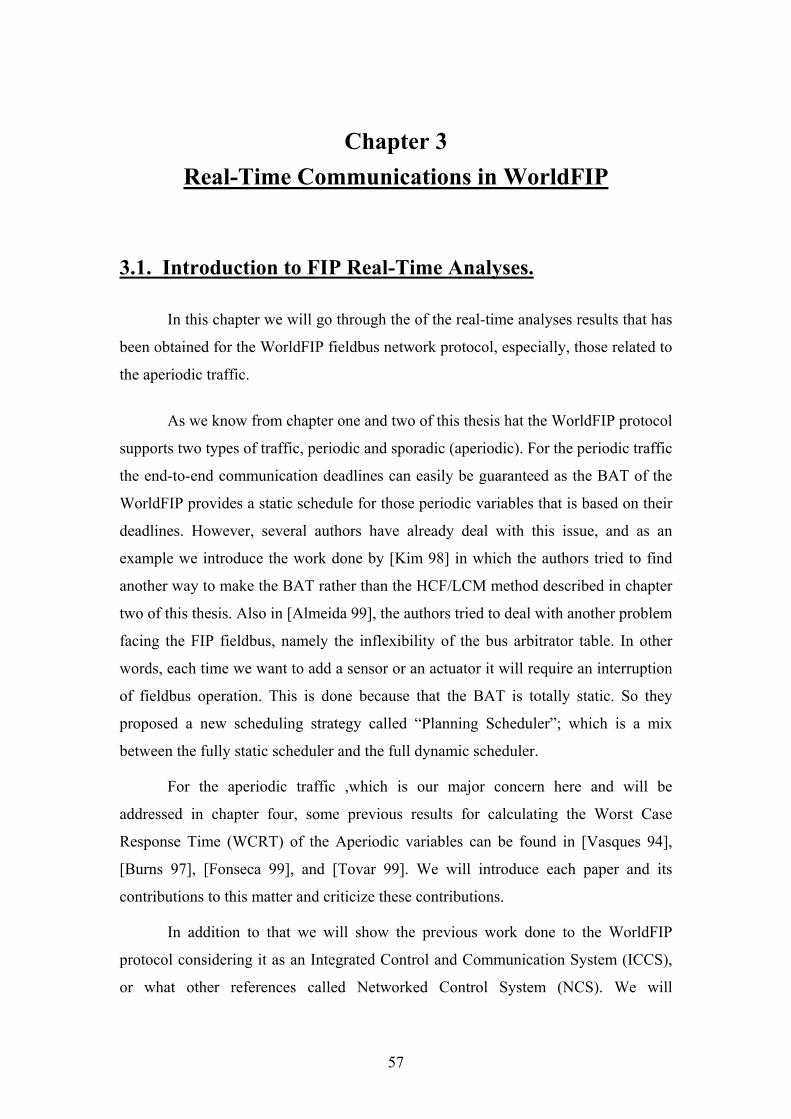
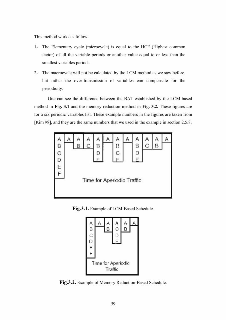
One can see the difference between the BAT established by the LCM-based

method in Fig. 3.1 and the memory reduction method in Fig. 3.2. These figures are

for a six periodic variables list. These example numbers in the figures are taken from

[Kim 98], and they are the same numbers that we used in the example in section 2.5.8.

Fig.3.1. Example of LCM-Based Schedule.

Fig.3.2. Example of Memory Reduction-Based Schedule.

60

The HCF/LCM BAT consists of twelve elementary cycles; each elementary

cycle is of five microseconds time length. The Memory-Reduced BAT consists of six

microcycles only and each microcycle consists of five microseconds as well. As we

see that the new BAT now become shorter than before, which means that they have

succeeded in reducing the amount of memory that is needed to store the BAT. In fact

the authors of [Kim 98] did not ignore this fact.

Also, we can see that this will make the network utilization (for the periodic

variables only) become higher, which means that there is less time available for the

aperiodic traffic. This will lead to longer worst case response time of the aperiodic

variables. What can be also noted about this method is that it can cause severe

communication jitter which in some cases the control applications affected by this

kind of jitter in catastrophic manner as Kim et al. stated in [Kim 98].

Another important drawback of this method is that the authors did not mention

clearly how to evaluate the macrocycle from the periodicities of the periodic

variables. Thus they left this to the trail and error. What is considered as evidence to

this, in [Kim 98] we find two proposed schedules for this method example.

3.2.2. The Jitter-Resolving Scheduling Method.

The second method Kim called it “jitter-resolving method”, in which he tried

to reduce the communication jitter. [Kim 98] stated that in some control applications

the jitter of the control loop input, and/or the jitter of the plant output(s) can have

critical effects on the control system. In this method he modified the periods of the

periodic FIP variables and made these variables harmonic before scheduling these

variables, and then he created the BAT using the ordinary HCF/LCM based method.

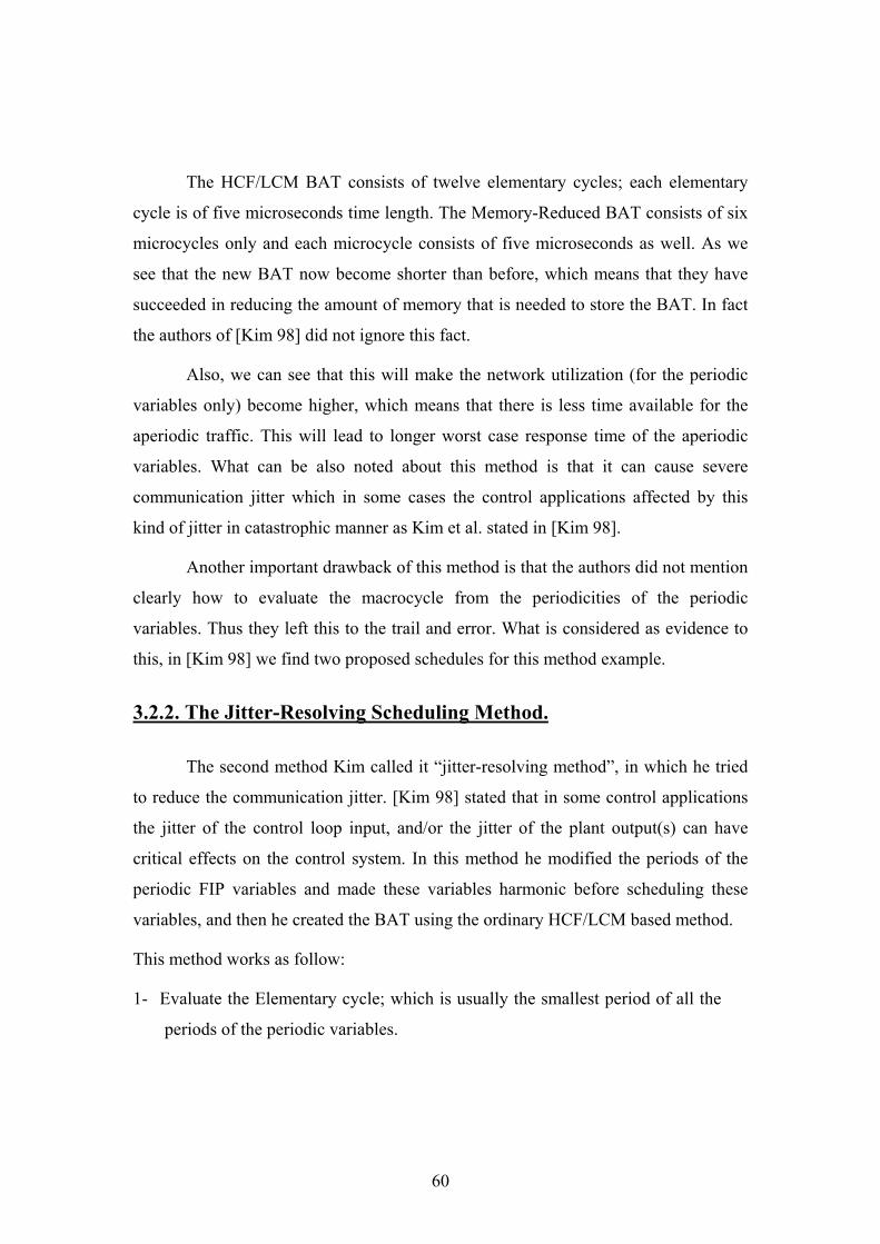
This method works as follow:

1- Evaluate the Elementary cycle; which is usually the smallest period of all the

periods of the periodic variables.

61

2- Now we find new values of the periods of the aperiodic variables, such that the

new value is equal to the largest multiple of the elementary cycle and is equal

to or less than the original period of the variables.

3- Construction of the BAT schedule is carried out using the LCM of all the new

periods we got from step two of this algorithm.

We now can see the resulting the BAT of this jitter-resolving method below in

Fig. 3.3.

Fig.3. 3. Example of Jitter-Resolving-Based Schedule.

There is no communication jitter in this method, because the intervals between

consecutive transmission times of each periodic variable are now equal. Also, it’s

worth noting that this method makes the network utilization very high (concerning the

periodic variables only), which at the end will lead to poor response time of the

aperiodic variables.

What we can see obviously is that the memory size that is required to store the

BAT in this method is so small. This means that this method serves both goals; which

are the jitter resolving and the memory reduction, at the same time. What is more

[Kim 98] mentioned that the network utilization of this method became higher than

that of the other two ways.

Fig. 3.4. shows a comparison between these three methods based on network

utilization, jitter time, and memory size [Kim 98]. As we can see from this figure, the

62

FIP BAT that was made by the HCF/LCM-based scheduling method is the most

appropriate method when constructing the BAT. Thus the HCF/LCM method is the

optimum method in scheduling the BAT. Why? Because HCF/LCM method has a

small amount of communication jitter, and its utilization is good as it leaves time to

serve the aperiodic traffic (unlike the other methods). The only disadvantage in the

HCF/LCM method is that its BAT is rather long. However since the BA is the most

important node in the network, we conclude that it must be a good computer with a

rather higher amount of memory than those of the ordinary producer/consumer nodes.

We will use the HCF/LCM-based BAT through this thesis (i.e. in both chapter four,

and chapter five).

Fig.3. 4. Performance Comparison between the Three Methods.

Finally we would like to add that these three methods are not the only

modification that done to the FIP's BAT on static bases. In fact there is another

statically modified BAT algorithm that was proposed by Hong in [Hong 95];

however, we will refer to this work mot as a new BAT scheduling scheme; but as it

addressed the stability of the closed loop control systems that are attached along the

FIP's network. For more information please refer to section 3.6. of this same chapter.

63

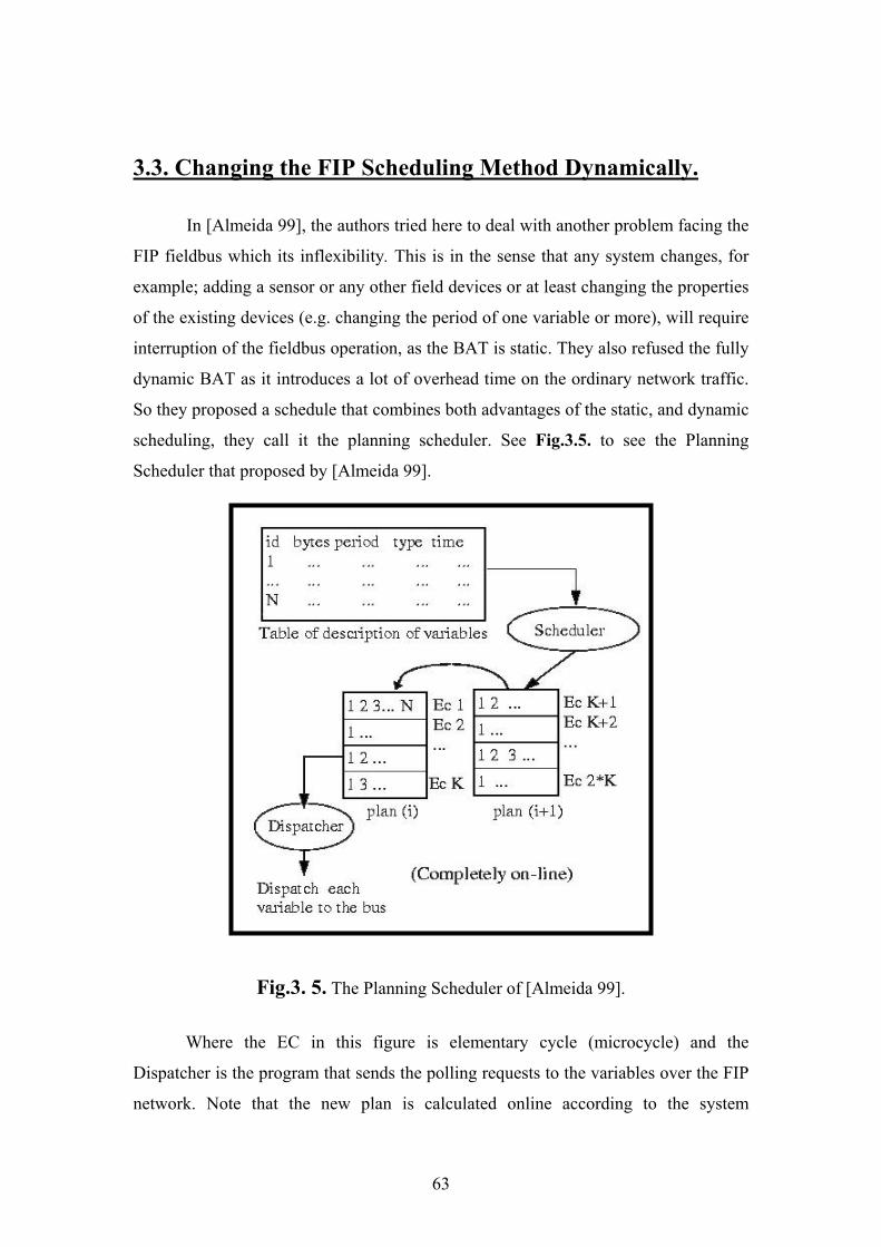
3.3. Changing the FIP Scheduling Method Dynamically.

In [Almeida 99], the authors tried here to deal with another problem facing the

FIP fieldbus which its inflexibility. This is in the sense that any system changes, for

example; adding a sensor or any other field devices or at least changing the properties

of the existing devices (e.g. changing the period of one variable or more), will require

interruption of the fieldbus operation, as the BAT is static. They also refused the fully

dynamic BAT as it introduces a lot of overhead time on the ordinary network traffic.

So they proposed a schedule that combines both advantages of the static, and dynamic

scheduling, they call it the planning scheduler. See Fig.3.5. to see the Planning

Scheduler that proposed by [Almeida 99].

Fig.3. 5. The Planning Scheduler of [Almeida 99].

Where the EC in this figure is elementary cycle (microcycle) and the

Dispatcher is the program that sends the polling requests to the variables over the FIP

network. Note that the new plan is calculated online according to the system

64

parameter change, and not offline. In other words, the new plans (BATs) are not

stored previously. The scheduler is the program (engine) that builds or calculates the

BAT (plan) given the table that describes the periodic variables properties. That table

is not fixed and can be changed. The dispatcher is the program that changes the BAT

construction every time the scheduler changes the plan.

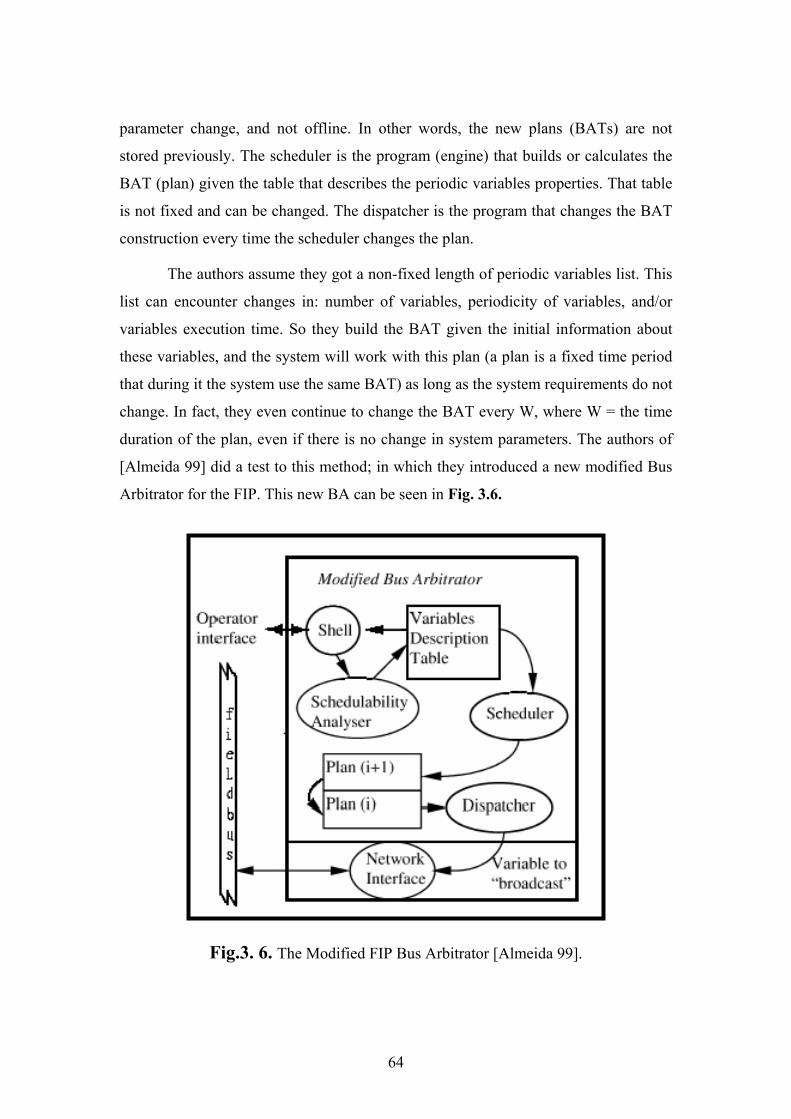
The authors assume they got a non-fixed length of periodic variables list. This

list can encounter changes in: number of variables, periodicity of variables, and/or

variables execution time. So they build the BAT given the initial information about

these variables, and the system will work with this plan (a plan is a fixed time period

that during it the system use the same BAT) as long as the system requirements do not

change. In fact, they even continue to change the BAT every W, where W = the time

duration of the plan, even if there is no change in system parameters. The authors of

[Almeida 99] did a test to this method; in which they introduced a new modified Bus

Arbitrator for the FIP. This new BA can be seen in Fig. 3.6.

Fig.3. 6. The Modified FIP Bus Arbitrator [Almeida 99].

65

The Scheduler Analyzer in the figure is a program that checks the schedule to

see if it will meet the Real-Time constraints or not. The Shell is the operating system

shell interface which the user uses to input the variables parameters into the Variables

Description Table.

Along they derived a sufficient Schedulability condition to overcome the old

inability of dynamic schedulers to guarantee the Schedulability of the variables for a

long system operation. What is more, they introduce a formula to calculate the

complexity of the calculation of the BAT with this new method [Almeida 99].

There are a few remarks that we can mention here about this new scheduling

algorithm. First of all, this new "Planner Scheduler" introduces an overhead to the

network (due to the online process of changing the plan) which induces a delay in the

control applications. This delay may not be accommodated (or compensated) by all

applications. We are fully aware that this delay may be lighter than that of the fully

dynamic scheduler. Second, from our point of view, the tests on this scheduler were

not on a real world factory or at least on a similar experimental setup model like the

one that was done by [Zhang 2001], but instead they tested it using simulation test bed

of three PC's using a cheap, and low bit rate bus.

Now after reviewing the scheduling policies and methods that were proposed

for the FIP protocol, we will now turn into another important Real-Time aspect; that is

calculating the Worst Case Response Time of the FIP aperiodic streams.

66

3.4. Calculating the WCRT of FIP Sporadic Streams.

There are many references that addressed the problem of calculating the Worst

Case Response Time of the aperiodic variables of the WorldFIP's. Examples of these

are [Vasques 94], [Burns 97], [Fonseca 99], [Tovar 99-1], and [Almeida 2002]. We

like to state that the latest paper (i.e. [Almeida 2002]) is simply slightly enhanced

version of [Tovar 99-1], so we will not talk directly about this paper as the main work

was done in [Tovar 99-1]. All these references did their work on one type of the

aperiodic variables; namely the Urgent aperiodic variables.

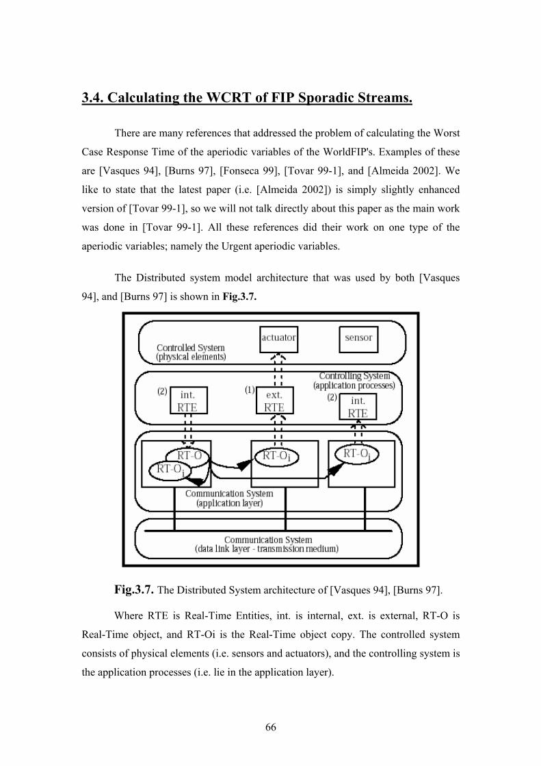
The Distributed system model architecture that was used by both [Vasques

94], and [Burns 97] is shown in Fig.3.7.

Fig.3.7. The Distributed System architecture of [Vasques 94], [Burns 97].

Where RTE is Real-Time Entities, int. is internal, ext. is external, RT-O is

Real-Time object, and RT-Oi is the Real-Time object copy. The controlled system

consists of physical elements (i.e. sensors and actuators), and the controlling system is

the application processes (i.e. lie in the application layer).

67

They assumed that the communication system high-level (in the application

layer) provides the service of transferring the time dependent information produced by

a producer (RT-O) to the different consumers where the copies in the consumer nodes

are called RT-O images: RT-Oi.

What is more, they assumed that the communication system in the lower level

or more precisely the Data Link Layer has to manage the sharing of the transmission

medium for the data packets exchanges. The frame exchanges schedulability is a hard

point, which must satisfy time constraints (resulting from the time constraints in the

higher layers).

In addition to that, they assumed that they had also other causes of information

exchanges between the nodes; such as: alarm occurrences and configuration definition

messages (which do not necessarily have time constraints).

They assumed that the variables streams of the FIP periodic are executed in

the following way:

• During the microcycle first phase, the B.A. induces a predefined sequence of

periodic variables exchange. During this phase, distant stations, if addressed, may

signalize to the B.A. for pending aperiodic variables requests (i.e. implicit

pooling). Explicit pooling is also possible but we will not consider this option1.

• In the following unused microcycle time (if any), the B.A. induces the exchange of

the pending aperiodic variables requests which have been previously made.

Both of [Vasques 94], and [Burns 97] did a pre-run-time schedulability

analysis to obtain the schedulability condition and then they calculated the WCRT of

the aperiodic urgent variables.

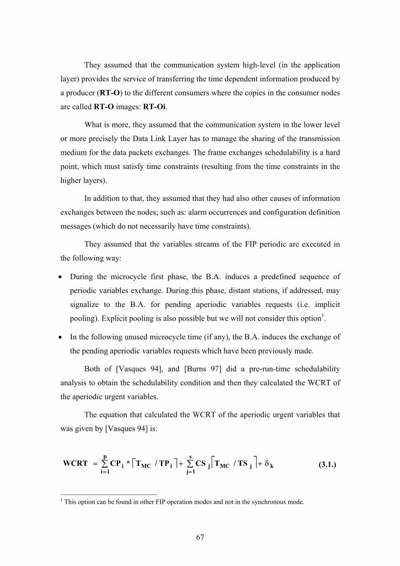
The equation that calculated the WCRT of the aperiodic urgent variables that

was given by [Vasques 94] is:

(3.1.)

1 This option can be found in other FIP operation modes and not in the synchronous mode.

ks

1jjMCj

p

1iiMCi TS/TCSTP/T*CPWCRT δ++= ∑∑

==

68

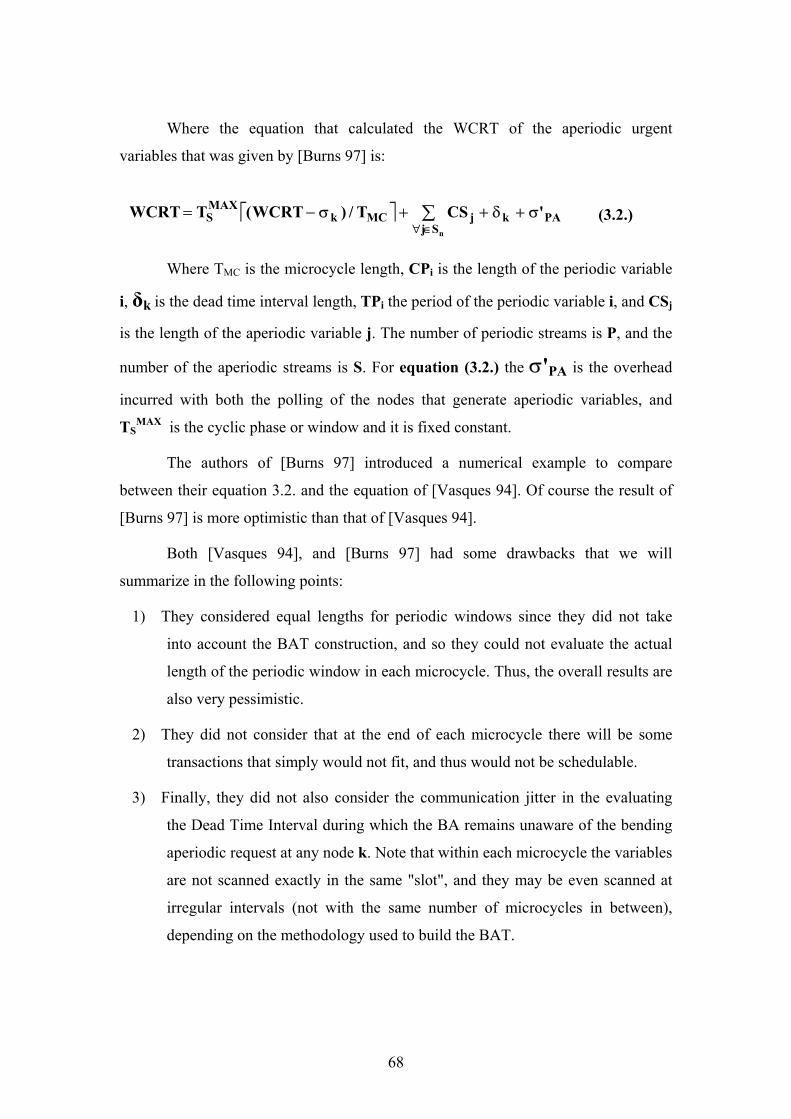
Where the equation that calculated the WCRT of the aperiodic urgent

variables that was given by [Burns 97] is:

(3.2.)

Where TMC is the microcycle length, CPi is the length of the periodic variable

i, δk is the dead time interval length, TPi the period of the periodic variable i, and CSj

is the length of the aperiodic variable j. The number of periodic streams is P, and the

number of the aperiodic streams is S. For equation (3.2.) the σ'PA is the overhead

incurred with both the polling of the nodes that generate aperiodic variables, and

TSMAX is the cyclic phase or window and it is fixed constant.

The authors of [Burns 97] introduced a numerical example to compare

between their equation 3.2. and the equation of [Vasques 94]. Of course the result of

[Burns 97] is more optimistic than that of [Vasques 94].

Both [Vasques 94], and [Burns 97] had some drawbacks that we will

summarize in the following points:

1) They considered equal lengths for periodic windows since they did not take

into account the BAT construction, and so they could not evaluate the actual

length of the periodic window in each microcycle. Thus, the overall results are

also very pessimistic.

2) They did not consider that at the end of each microcycle there will be some

transactions that simply would not fit, and thus would not be schedulable.

3) Finally, they did not also consider the communication jitter in the evaluating

the Dead Time Interval during which the BA remains unaware of the bending

aperiodic request at any node k. Note that within each microcycle the variables

are not scanned exactly in the same "slot", and they may be even scanned at

irregular intervals (not with the same number of microcycles in between),

depending on the methodology used to build the BAT.

PAkSj

jMCkMAXS 'CST/)WCRT(TWCRT

n

σ+δ++σ−= ∑∈∀

69

The analysis that was presented in [Tovar 99-1] improved the previous work

of [Burns 97] considering all of the three above mentioned aspects in an integrated

manner. What is more [Tovar 99-1] presented methodologies for building the

WorldFIP BAT, and thus performing an integrated analysis for both the periodic and

aperiodic traffic. We will leave the details and the assumptions of this model to

chapter 4 of this thesis as it is almost the same model that we adapt in calculating the

WCRT.

But [Tovar 99-1], and later in [Almeida 2002] also had some drawbacks that

we would like to summarize them in the following points:

1- They assume that when a station sends for aperiodic transfer, that there is only

one aperiodic variable; but as we saw from the WorldFIP protocol, the

(RP_RQ) frame can contain a list up to 64 variable identifiers [FIP 98].

2- They did not take into account the queues sizes of the BA (there are two

queues for the Urgent sporadic variables transfer, two for the Normal sporadic

variables transfer, one for the Unacknowledged sporadic message transfer,

and one for the Acknowledged sporadic message transfer).

3- They did not mention how to calculate the maximum number of the urgent

aperiodic variables existing in the FIP network (they call it NA). Even if we

consider that this number is system a parameter that to be known at setup the

time, it still be changed during the operation time. We will see in chapter 4 in

this thesis that there is no need to calculate this number, or even to know its

value. The method that we will introduce is independent of this number.

4- They did not find the WCRT of the Normal sporadic variables or the aperiodic

messages.

At last we would like to mention that the work that was done by [Fonseca 99], the

authors took into account the padding frames, which are used in the FIP network to

maintain synchronization of the microcycles. But the formula they presented was the

same formula that was used by [Burns 97], which we criticized before. We will

propose a new formula to correct all these drawbacks in chapter 4 of this thesis and

verify it using the WorldFIP traffic simulation engine that we developed.

70

3.5. The Stability of FIP Control Loops.

There are many papers that addressed the stability of the fieldbus's associated

control loops that share the same medium [Halevi 88] [Shin 92] [Hong 95] [Zhang

2001] [Walsh 2001]. In these models the sensor/actuator terminal in one control loop

is communicating with the controller terminal via a digital bus or the fieldbus

network. These models can be divided into two main categories; in the first category

the controller node is central for all the control closed loop systems, while in the

second category each control loop has its own controller. We will review each of

these two categories in detail.

In both categories, each terminal suffers from time-variable delays when

accessing the bus. These delays come from two sources; one from other traffic that is

running on the network bus, and the second from the low frequency that most of the

sensors operate on [Halevi 88]. The network induced delay causes degradation in the

performance of the closed-loop system, or may further lead to system instability.

Many solutions were proposed to solve the delay problem. One solution was to find

new values of the sampling times of the control loops attached on the fieldbus that can

compensate for the network delay [Halevi 88] [Hong 95]. Other solutions were

dedicated only towards finding the maximum or the supreme value of this delay that

keeps the closed loop control system stable [Zhang 2001] [Walsh 2001]. We will

review each of these two solutions shortly after in detail. We will call the first

solution: the effect of network delay on control loop stability, and the second solution

determination of sampling periods of the control loops.

3.5.1. Effect of Network Delay on the Control Loop Stability.

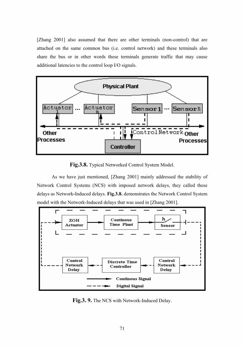
Fig. 3.8. shows the fieldbus system model that Zhang et. al. used in their

paper, also [Walsh 2001] adapted the same model approximately. In this figure the

authors of [Zhang 2001] assumed that there is only one digital controller that is

attached to the fieldbus network, with "m" actuators and "n" sensors. They call this

system as Networked Control System or NCS. These actuators/sensors are attached

via the common bus to that controller, and directly attached to the physical plant.

71

[Zhang 2001] also assumed that there are other terminals (non-control) that are

attached on the same common bus (i.e. control network) and these terminals also

share the bus or in other words these terminals generate traffic that may cause

additional latencies to the control loop I/O signals.

Fig.3.8. Typical Networked Control System Model.

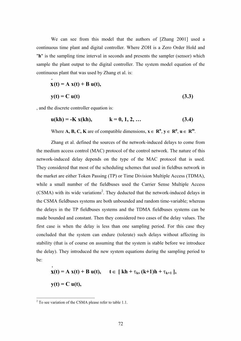
As we have just mentioned, [Zhang 2001] mainly addressed the stability of

Network Control Systems (NCS) with imposed network delays, they called these

delays as Network-Induced delays. Fig.3.8. demonstrates the Network Control System

model with the Network-Induced delays that was used in [Zhang 2001].

Fig.3. 9. The NCS with Network-Induced Delay.

72

We can see from this model that the authors of [Zhang 2001] used a

continuous time plant and digital controller. Where ZOH is a Zero Order Hold and

"h" is the sampling time interval in seconds and presents the sampler (sensor) which

sample the plant output to the digital controller. The system model equation of the

continuous plant that was used by Zhang et al. is:

(t) = A x(t) + B u(t),

y(t) = C u(t) (3.3)

, and the discrete controller equation is:

u(kh) = -K x(kh), k = 0, 1, 2, … (3.4)

Where A, B, C, K are of compatible dimensions, x ∈ Rn, y ∈ Rp, u ∈ Rm.

Zhang et al. defined the sources of the network-induced delays to come from

the medium access control (MAC) protocol of the control network. The nature of this

network-induced delay depends on the type of the MAC protocol that is used.

They considered that most of the scheduling schemes that used in fieldbus network in

the market are either Token Passing (TP) or Time Division Multiple Access (TDMA),

while a small number of the fieldbuses used the Carrier Sense Multiple Access

(CSMA) with its wide variations2. They deducted that the network-induced delays in

the CSMA fieldbuses systems are both unbounded and random time-variable; whereas

the delays in the TP fieldbuses systems and the TDMA fieldbuses systems can be

made bounded and constant. Then they considered two cases of the delay values. The

first case is when the delay is less than one sampling period. For this case they

concluded that the system can endure (tolerate) such delays without affecting its

stability (that is of course on assuming that the system is stable before we introduce

the delay). They introduced the new system equations during the sampling period to

be:

(t) = A x(t) + B u(t), t ∈ [ kh + τk, (k+1)h + τk+1 ],

y(t) = C u(t),

2 To see variation of the CSMA please refer to table 1.1.

.x

.x

73

u(t+) = -K x(t - τk), t ∈ [ kh + τk, k = 0, 1, 2, … ] (3.5)

Now; sampling the system with period "h" the new system equations with

network-induced delay "τ" are:

x((k+1)h) = Φ x(kh) + Γ0 (τk) u(kh) + Γ1(τk) u((k-1)h),

y(kh) = C x(kh) (3.6.)

Where

Φ = eAh

Γ0 (τk) =

Γ1(τk) =

they defined the augmented state vector to be:

z ((k + 1) h) = (k) z(kh) (3.7.)

where

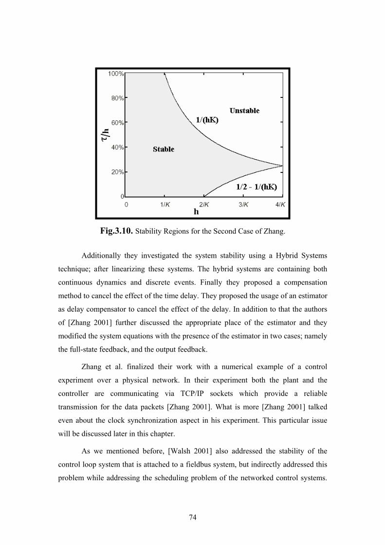
The second case is when the delay is more than one sampling time. For this

case the authors of [Zhang 2001] derived the stability regions for the networked

control system transfer function design for the first order integrator case. They plotted

the stability regions between the system sampling period "h", and the normalized

network-induced delay "τ/h". This can be seen in Fig. 3.10. We shaded the system

stability regions in light gray.

∫τ− kh

0As ,Bdse

∫ τ−hh

Ask

,Bdse

−

τΓτΓ−Φ=Φ

0K)(K)( k1k0~

~Φ

74

Fig.3.10. Stability Regions for the Second Case of Zhang.

Additionally they investigated the system stability using a Hybrid Systems

technique; after linearizing these systems. The hybrid systems are containing both

continuous dynamics and discrete events. Finally they proposed a compensation

method to cancel the effect of the time delay. They proposed the usage of an estimator

as delay compensator to cancel the effect of the delay. In addition to that the authors

of [Zhang 2001] further discussed the appropriate place of the estimator and they

modified the system equations with the presence of the estimator in two cases; namely

the full-state feedback, and the output feedback.

Zhang et al. finalized their work with a numerical example of a control

experiment over a physical network. In their experiment both the plant and the

controller are communicating via TCP/IP sockets which provide a reliable

transmission for the data packets [Zhang 2001]. What is more [Zhang 2001] talked

even about the clock synchronization aspect in his experiment. This particular issue

will be discussed later in this chapter.

As we mentioned before, [Walsh 2001] also addressed the stability of the

control loop system that is attached to a fieldbus system, but indirectly addressed this

problem while addressing the scheduling problem of the networked control systems.

75

Like [Zhang 2001], Walsh et al. also used the same model of one control loop over

the fieldbus network. However, they focused in their study on the famous CAN

fieldbus protocol. Then they studied the effect of the scheduling method over the

closed loop system stability as the scheduling method introduced delays in the

transmission of the signals over the bus. They continued the study to find delay

bounds which they called a "Dynamic Scheduler Error Bound" and "Static Scheduler

Error Bound". At last the authors used these results to derive the stability condition of

the NCS model.

Walsh et. al. also proposed a free of queue fieldbus system (i.e. to make the

fieldbus system without any queues). They called this method as Try Once Discard

(TOD) as the node that has the data packet sample will discard the data if the network

is not available yet and hence, the node which waits for this data will use the old data

packet sample.

At the end, they proposed a stability theory for the NCS with the same model

that was used by [Zhang 2001] and its Equations are (3.3.) and (3.4.). In this theory;

the authors finds a maximum allowable delay that keeps the Networked Control

System globally exponentially stable [Walsh 2001]. [Walsh 2001] verified their work

using two famous examples. The first example is the Batch Reactor Experiment and

sketched the results of its simulation. The other example that they used is the Dryer

Experiment.

As we stated before the authors of [Walsh 2001] used the famous CAN

fieldbus protocol in the data packets transmission over the bus; however, they claimed

that their work can fit with any other fieldbus protocol without the need for further

modification. They stated that their work can be extended further to include many

closed- loop control systems.

3.5.2. Determination of Sampling Periods of The Control Loops.

A different view was taken by both [Hong 95], [Halevi 88], who both used the

results of the variable-time-delay control system stability criteria, that was presented

in [Hirai 80], to find a suitable way to assign values to the sampling times (i.e.

76

periods) of the control system loops attached to the fieldbus. They both divide the

overall delay of the control loop into two components; namely the controller to

actuator delay and the sensor to controller delay. What is more, they did not combine

these two components into one equivalent overall delay. They justified this situation

by concluding that these two delays are different in nature and properties. We would

like to add that the work of [Hong 95] was also inspired by [Shin 92], [Schwartz 88],

and [Ray 88]. Although the authors of [Halevi 88] were interested in finding both the

maximum allowable delay of each control loop and the model that can best describe

the delays associated with the ICCS's, [Hong 95] used the results of [Halevi 88] and

[Hirai 80] to concentrate on finding a scheduling algorithm of the fieldbus to maintain

certain performance metric to all the closed-loops that are attached to the system bus.

This is done while [Hong 95] tried to preserve the maximum utilization of the system

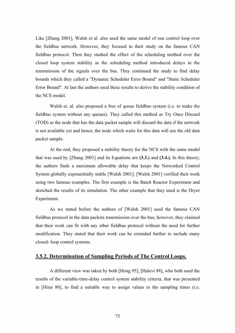
bus. See Fig. 3.11. to see the Integrated Communication and Control System (ICCS)

model that [Halevi 88] used in his paper.

Fig.3.11. The Schematic Diagram of the ICCS of [Halevi 88].

77

What is worth noting in [Hong 95] is that the author did not take into account

the sporadic (aperiodic) traffic of the fieldbus system (neither did [Halevi 88]).

Despite this, the work of [Hong 95] can be applied to the centralized systems like the

FIP protocol with some modifications as we will see later in chapter 5 of this thesis.

As we will see later in chapter five, when Hong did not take into account the

aperiodic traffic plus the overvaluing of the system bus periodic utilization all this

made the worst case response time of the aperiodic traffic extremely high. Of course,

we tried to correct this situation, as the aperiodic WCRT is important to us, by

modifying the scheduling algorithm one more time to free more time for the aperiodic

traffic, while preserving the overall system stability at the same time.

Finally, we used the Matlab Simulink to justify our new algorithm using the

same closed-loop control system example that was used by [Hong 95] with only slight

changes. We would like to state here that the author of [Hong 95] did not mention

how exactly he verified his work, or in other words, what the system properties he

used to justify his work are.

78

3.6. WorldFIP Clock Synchronization.

3.6.1. Why the Clock Synchronization?

Here we would like to introduce another important real-time aspect, which is

the clock synchronization of FIP system. The importance of clock synchronization

came from the need to verify the information validity. WorldFIP provides information

validity via promptness and refreshments statuses (as we saw in chapter 2). So the

setting of these timers, that are the refreshment and promptness timers, is important.

3.6.2. Clock Synchronization from the Application Layer

What is also worth noting for this particular case is that [Kim 98] addressed

the clock synchronization in FIP environment. In fact [Kim 98] proposed a

synchronization mechanism that based on clock mechanism. [Kim 98] argued that the

promptness and refreshment status are not sufficient to guarantee the end-to-end

deadline of the periodic variables by themselves. So Kim et. al. in [Kim 98] demanded

that the synchronization between the application processes and the network should be

well established in order to guarantee the validity of information.

In his proposed method [Kim 98] set the phase of certain process (PHi) to

equal to the maximum periodic information transmission time among all the

microcycles, the refreshment timer value to equal to the deadline of the same process,

and the promptness timer to equal to the deadline of the same process. Where the

deadline itself of this particular process is equal the difference between the period of

transmission of information and the maximum periodic information transmission time

among all the microcycles. In addition, this synchronization is done between the

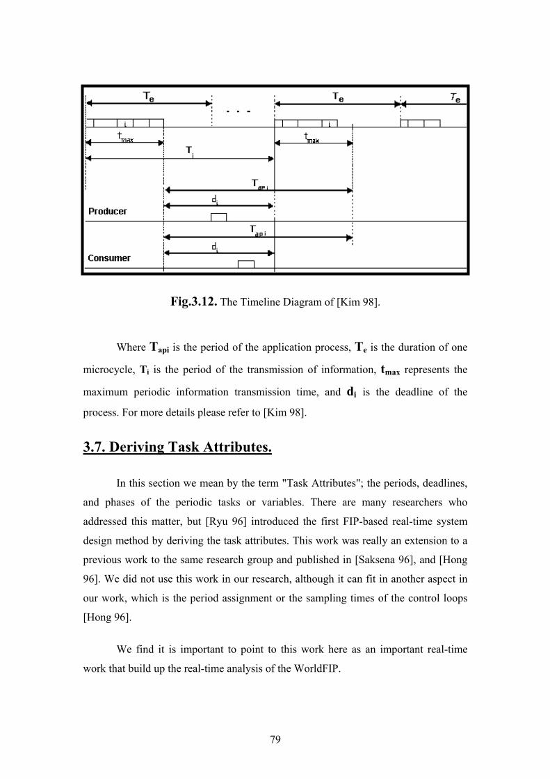
producer node, and the consumer node. Fig. 3.12. shows the time line diagram of this

proposed clock synchronization.

79

Fig.3.12. The Timeline Diagram of [Kim 98].

Where Tapi is the period of the application process, Te is the duration of one

microcycle, Ti is the period of the transmission of information, tmax represents the

maximum periodic information transmission time, and di is the deadline of the

process. For more details please refer to [Kim 98].

3.7. Deriving Task Attributes.

In this section we mean by the term "Task Attributes"; the periods, deadlines,

and phases of the periodic tasks or variables. There are many researchers who

addressed this matter, but [Ryu 96] introduced the first FIP-based real-time system

design method by deriving the task attributes. This work was really an extension to a

previous work to the same research group and published in [Saksena 96], and [Hong

96]. We did not use this work in our research, although it can fit in another aspect in

our work, which is the period assignment or the sampling times of the control loops

[Hong 96].

We find it is important to point to this work here as an important real-time

work that build up the real-time analysis of the WorldFIP.

80

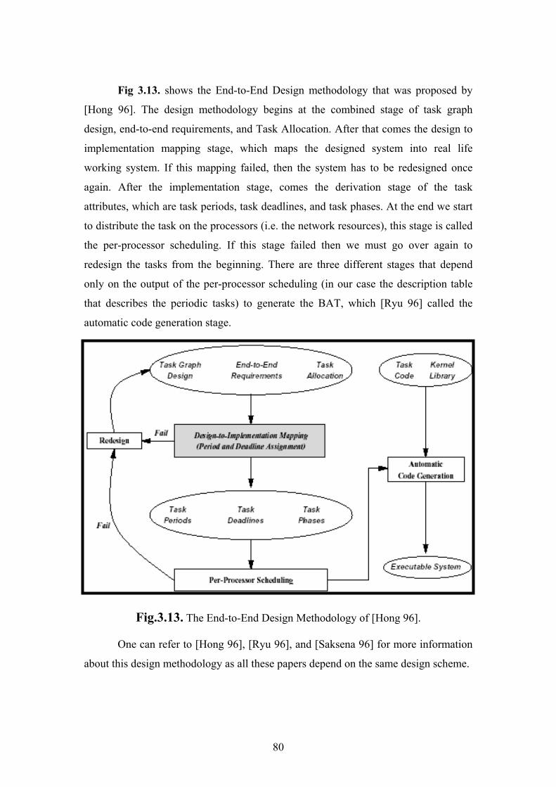
Fig 3.13. shows the End-to-End Design methodology that was proposed by

[Hong 96]. The design methodology begins at the combined stage of task graph

design, end-to-end requirements, and Task Allocation. After that comes the design to

implementation mapping stage, which maps the designed system into real life

working system. If this mapping failed, then the system has to be redesigned once

again. After the implementation stage, comes the derivation stage of the task

attributes, which are task periods, task deadlines, and task phases. At the end we start

to distribute the task on the processors (i.e. the network resources), this stage is called

the per-processor scheduling. If this stage failed then we must go over again to

redesign the tasks from the beginning. There are three different stages that depend

only on the output of the per-processor scheduling (in our case the description table

that describes the periodic tasks) to generate the BAT, which [Ryu 96] called the

automatic code generation stage.

Fig.3.13. The End-to-End Design Methodology of [Hong 96].

One can refer to [Hong 96], [Ryu 96], and [Saksena 96] for more information

about this design methodology as all these papers depend on the same design scheme.

81

The authors of [Ryu 96] mainly addressed the derivation of the timing

constraints of the FIP system. They meant by the timing constraints the period

assignment and the phase/deadline assignment.

They divided the constraints associated to the period assignment into two

major categories, the range constraints, and the harmonicity constraints.

The range constraints are to ensure the minimum rate of task executions. This

leads to impose an upper-bound on the periods. As for the harmonicity constraints, are

arising from synchronous communication between each producer/consumer task pair.

For the phase/deadline assignment he considered two factors, the task response Time,

and the scheduling policy. The task response is the direct metric for the schedulability

of the task. The scheduling policy is responsible for changing the response time of the

task. Finally [Ryu 96] introduced the performance evaluation of his proposed system.