Chapter 3 PROTON SOURCE - Advanced Accelerator · PDF file124 CHAPTER 3. PROTON SOURCE...
25
Chapter 3 PROTON SOURCE Contents 3.1 Requirements .............................. 123 3.2 Production of Short Bunches .................... 126 3.3 Stability During Acceleration .................... 130 3.4 Stability of Short Bunches ...................... 132 3.5 Components .............................. 134 3.6 Examples ................................ 137 3.6.1 30 GeV ................................. 137 3.6.2 10 GeV ................................. 138 3.6.3 2.5 Hz .................................. 139 3.6.4 Polarized μ Production ........................ 140 3.7 R & D Issues .............................. 140 3.1 Requirements The proton driver requirements are determined by the design luminosity of the collider, and the efficiencies of muon collection, cooling, transport and acceleration. These numbers are shown in Table 3.1. In addition to accelerating a large charge, the machines must operate at high repetition rates, which are determined by the μ lifetime at high energies and the overall power minimization in the accelerator systems. The rms bunch length for protons on target has been set at 1 ns to: 1) minimize the initial longitudinal emittance of μ’s entering the cooling system, and 2) optimize the separation of the populations of + and 123
Transcript of Chapter 3 PROTON SOURCE - Advanced Accelerator · PDF file124 CHAPTER 3. PROTON SOURCE...

Chapter 3
PROTON SOURCE
Contents
3.1 Requirements . . . . . . . . . . . . . . . . . . . . . . . . . . . . . . 123
3.2 Production of Short Bunches . . . . . . . . . . . . . . . . . . . . 126
3.3 Stability During Acceleration . . . . . . . . . . . . . . . . . . . . 130
3.4 Stability of Short Bunches . . . . . . . . . . . . . . . . . . . . . . 132
3.5 Components . . . . . . . . . . . . . . . . . . . . . . . . . . . . . . 134
3.6 Examples . . . . . . . . . . . . . . . . . . . . . . . . . . . . . . . . 137
3.6.1 30 GeV . . . . . . . . . . . . . . . . . . . . . . . . . . . . . . . . . 137
3.6.2 10 GeV . . . . . . . . . . . . . . . . . . . . . . . . . . . . . . . . . 138
3.6.3 2.5 Hz . . . . . . . . . . . . . . . . . . . . . . . . . . . . . . . . . . 139
3.6.4 Polarized µ Production . . . . . . . . . . . . . . . . . . . . . . . . 140
3.7 R & D Issues . . . . . . . . . . . . . . . . . . . . . . . . . . . . . . 140
3.1 Requirements
The proton driver requirements are determined by the design luminosity of the collider, and
the efficiencies of muon collection, cooling, transport and acceleration. These numbers are
shown in Table 3.1. In addition to accelerating a large charge, the machines must operate
at high repetition rates, which are determined by the µ lifetime at high energies and the
overall power minimization in the accelerator systems. The rms bunch length for protons
on target has been set at 1 ns to: 1) minimize the initial longitudinal emittance of µ’s
entering the cooling system, and 2) optimize the separation of the populations of + and
123

124 CHAPTER 3. PROTON SOURCE
− polarizations off the target, see Section 11.2.1, and Figure 11.7. Since the collection of
polarized µ’s is inefficient, we assume the proton driver must eventually provide an additional
factor of approximately two to compensate for the inefficiency in producing these beams.
An additional requirement is that the proton driver system must have low losses, to permit
inexpensive maintenance of components.
Table 3.1: Proton Driver Requirements
30 GeV 10 GeV
Rep. Rate 15 30 Hz
Protons 1014 1014 /pulse
Bunches 4 2 at target
Protons 2.5× 10¹³ 5× 10¹³ /bunch
The proton driver needs to deliver very narrow, high intensity proton bunches for the pion
production target. The main requirements for the driver were listed in Tb. 1 in the Intro-
duction. Note that this amounts to 7 MW of beam power in the proton beam. This level of
beam power is much higher than what is currently available at proton accelerators. However,
many detailed proposals have been worked out for multi-GeV hadron facilities or neutron
spallation sources that can achieve similar levels of beam power. For our requirements, the
designs for the KAON facility, which is a 30 GeV, 3 MW machine and a combination of the
BNL 5 MW spallation neutron source (SNS), and the ANL 10 GeV SNS design are most
appropriately used as the starting point for the design of the muon collider proton driver.
Table 3.2: Linac parameters
µµ Collider BNL-SNS
Max. Energy 0.6 0.6 GeV
Rep. Rate 15 60 Hz
Trans Emittance [95 %] 2.4 2.4 π mmmrad
Tot. Energy Spread 2.4 2.4 MeV
There are many ways of achieving the required beam intensities and power, (see Fig 3.1).
Tbs. 3.2, 3.3, 3.4 show one possible set of parameters for a proton driver consisting of a
600 MeV linac, a 3.6 GeV Booster and a 30 GeV Driver. Both the Booster and Driver
would operate at a repetition rate of 15 Hz with a total of four bunches with 0.25 × 10¹⁴
protons per bunch. The relatively low repetition rate of both Booster and Driver makes it
possible to use a metallic vacuum chamber with eddy current correction coils.[1] Both Linac

3.1. REQUIREMENTS 125
Table 3.3: Booster parameters
µµ Collider BNL-SNS
Injection Energy 0.6 0.6 GeV
Max. Energy 3.6 3.6 GeV
Rep. Rate 15 30 Hz
Protons per Pulse 1 × 10¹⁴ 1.45× 10¹⁴
Number of Bunches 4 2
Circumference 360 360 m
Trans. Emittance [95 %] 260 260 π mmmrad
Inc. Tune Shift Inj 0.25 0.25
rf Voltage per Turn 400 400 kV
rf Frequency (h=4) 2.62-3.24 1.31-1.62 MHz
Long. Emittance [95 %] 2 4 eVs
Table 3.4: Driver Parameters
µµ Collider AGS KAON
Injection Energy 3.6 1.5 3 GeV
Max. Energy 30 24 30 GeV
Rep. Rate 15 1 10 Hz
Protons per Pulse 1× 10¹⁴ 0.6× 10¹⁴ 0.6× 10¹⁴
Number of Bunches 4 8 225
Circumference 1080 800 1078 m
Transition Gamma 38 8.8 30 i
Max. Dispersion 2.3 m 2.2 m 7.4 m
Trans. Emittance [95%] 260 100 100 π mm mrad
Inc. Tune Shift Inj .10 .10 .10
RF Voltage per Turn 4 0.4 2.6 MV
Harmonic Number 12 8 225
RF Frequency 3.24-3.33 2.77-3.00 60.8-62.5 MHz
Long. Emittance [95 %] < 4.5 4.5 0.2 eVs
and Booster designs are copied from the BNL SNS design[2] with the only difference being
a lower repetition rate (15 Hz instead of 30 Hz), and a lower number of protons per pulse
(1 × 10¹⁴ instead of 1.45 × 10¹⁴). The Driver design is based on the experience with the
AGS and on the Japanese hadron Project (JHP)[3] and KAON[4] Driver design. The Driver
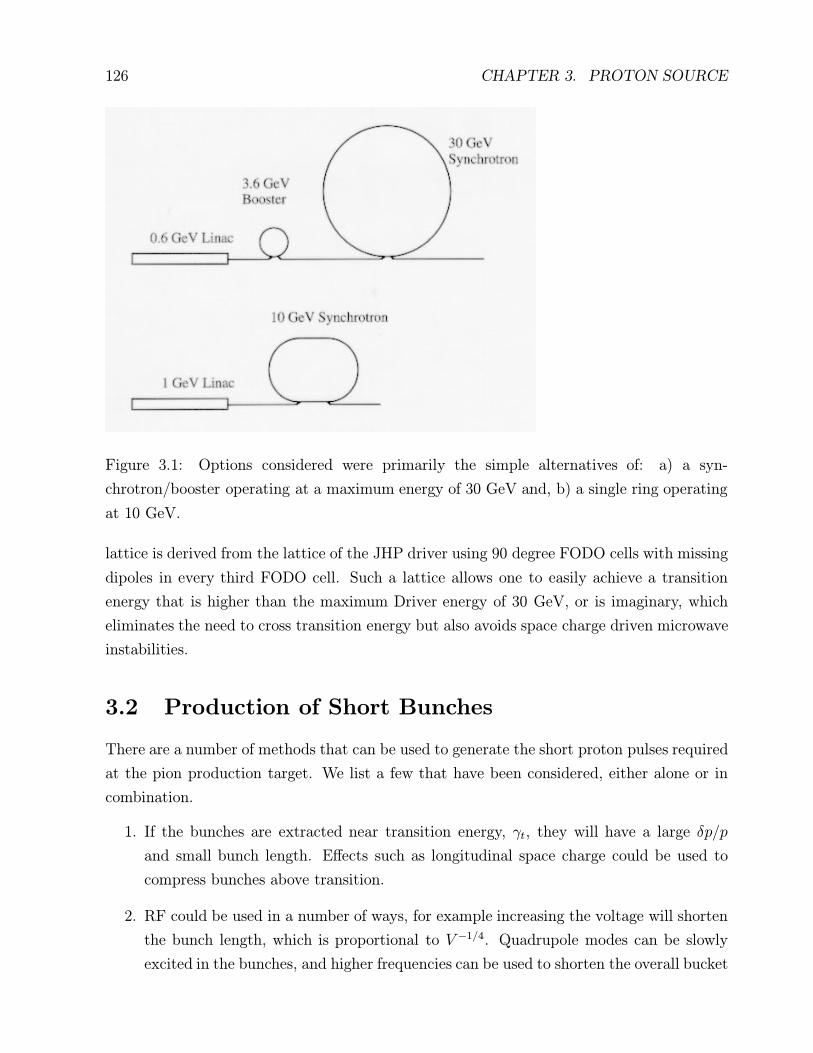
126 CHAPTER 3. PROTON SOURCE
Figure 3.1: Options considered were primarily the simple alternatives of: a) a syn-
chrotron/booster operating at a maximum energy of 30 GeV and, b) a single ring operating
at 10 GeV.
lattice is derived from the lattice of the JHP driver using 90 degree FODO cells with missing
dipoles in every third FODO cell. Such a lattice allows one to easily achieve a transition
energy that is higher than the maximum Driver energy of 30 GeV, or is imaginary, which
eliminates the need to cross transition energy but also avoids space charge driven microwave
instabilities.
3.2 Production of Short Bunches
There are a number of methods that can be used to generate the short proton pulses required
at the pion production target. We list a few that have been considered, either alone or in
combination.
1. If the bunches are extracted near transition energy, γt, they will have a large δp/p
and small bunch length. Effects such as longitudinal space charge could be used to
compress bunches above transition.
2. RF could be used in a number of ways, for example increasing the voltage will shorten
the bunch length, which is proportional to V −1/4. Quadrupole modes can be slowly
excited in the bunches, and higher frequencies can be used to shorten the overall bucket

3.2. PRODUCTION OF SHORT BUNCHES 127
length. Bunch rotation should be simpler and faster however. Bunches can be flattened
by slowly decreasing the voltage or placing the bunch in the unstable fixed point and
then rotated with increased voltage. Bunch rotation can be either a single process, or
taken in two steps, with energy shear near γt and a separate time shear done further
from γt.
3. Bunch shortening instabilities, driven by an inductive wall, could be excited by chang-
ing the wall impedance, perhaps by unbiasing ferrite.
4. Large numbers of bunches could be coalesced in an internal ring, or low frequency rf
linacs, probably induction linacs, can be used to generate a long energy ramp which
will coalesce in an external ring or long beam line.
5. Kickers and chicane systems could be used to take a finite number of equal energy
proton bunches over different paths to meet at the target.
6. Many short µ bunches could be combined to form a single intense bunch in the µ
cooling system.
The simplest option seems to be to extract near γt, However it is not clear that the
extracted bunches could be made sufficiently short to provide a 1 ns bunch length. Exper-
iments with bunches of 1013 protons have been kept circulating for periods of 100 ms with
values of η = 0.0005, with no losses, no negative mass instability, and good agreement with
theoretical predictions[5] The negative mass instability was seen in that part of the beam
which was above transition, but not in the part of the bucket below transition energy. The
stability of unbunched beams near transition has also been studied near transition at the
FermiLab antiproton accumulator. [6] Bunching near transition would require that the mo-
mentum spread at extraction would be large, however if the final energy of the accelerator
is large enough, the fractional momentum spread δp/p can, in principle, be accommodated
fairly easily at 30 GeV and with some difficulty, at 10 GeV.
Chicane systems can be used to generate a single pulse from a finite number of pulses,
however conservation of phase space requires that the bunches cannot be exactly in time
and collinear at the exit of such a system. In addition, the total length of chicane beamlines
must be roughly (n− 1/2) times the initial maximum separation of bunches.
Bunch Rotation Bunch rotation seems to offer the most reliable procedure for producing
short bunches and these methods have been studied in some detail. The longitudinal emit-
tance of the beam, εL, seems to be more or less independent of injection energy, repetition

128 CHAPTER 3. PROTON SOURCE
rate and other parameters for a variety of accelerators, with εL = 1 eV-s/1013 protons, see
Table 3.5. In general, the charge/pulse is more closely related to the transverse admittance,
and εL should not be directly related to factors which determine the maximum current limit
of the machine.
Table 3.5: Longitudinal Phase Space
protons/b εL [eV-s] p/eV-s
IPNS II 1.0× 10¹⁴ 7.5 1.3× 10¹³
BNL-SNS 7.5× 10¹³ 4.0 1.8× 10¹³
ISIS(inj) 2.0× 10¹³ 2.0 1.0× 10¹³
FNAL 5.0× 10¹² 2.0 2.5× 10¹²
IPNS 3.0× 10¹² 0.4 7.5× 10¹²
KAON 1.5× 10¹² 0.06 2.5× 10¹³
BNL-Booster 1.4× 10¹³ 2.0 9.6× 10¹²
Assuming 2.5× 10¹³ protons/bunch, this would imply εL = 2.5 eV-s at injection. When
the beam had reached the extraction energy, we require that the bunch length for 4 σ would
be 4 ns, however that would imply a momentum spread of 0.06 at 10 GeV and 0.02 at
30 GeV. Although both these numbers are larger than the momentum admittance of most
synchrotrons, the debuncher ring of the antiproton source at FermiLab, which operates at 8
GeV, accepts a ∆p/p > 0.05 and contains this beam for a much longer time than the few
turns the short, large momentum spread bunch will circulate in the driver synchrotron.
A common feature of many methods is that the bunch compression is a function of the
momentum spread δp/p and the momentum dependence of path lengths. The time required
for this compression is
tb =φrf
2π frf η δp/p, (3.1)
and is proportional to the required rf phase change, φrf , and inversely proportional to the rf
frequency, frf , slip factor, η, and the momentum spread, δp/p. Because of the large currents
involved, it is desirable to bunch as quickly as possible to avoid problems with instabilities.
Nevertheless coalescence of bunches spread around the circumference might require on the
order of 10 - 20 ms in a typical ring. Thus small compressor rings, which could accommodate
large η and δp/p could be used with induction linacs which would produce a large and linear
spread in the energies from front to back in a bunch, or train of bunches.
The bunching time is a function both of the beam energy γ and the difference between
the beam and transition energies, γt − γ. Because the machine circumference, η and δp/p

3.2. PRODUCTION OF SHORT BUNCHES 129
are dependent on the beam momentum, the bunching time goes like pn, with the exponent
n close to 4, depending on the assumptions used to determine the machine circumference
and rf frequency. Thus lower energy rings will have much faster bunching times than high
energy rings.
Two methods of bunch rotation have been considered. Decreasing the rf voltage to spread
the bunch out in time, followed by rotation, can be done for either a single bunch or a number
of smaller bunches using a subharmonic, (see Fig. 3.2)[7]. Since the process is nonlinear for
large amplitudes, the primary limitation is the initial phase angle which can be rotated into
the required bunch length. For an rf frequency of 3 MHz, the maximum rf phase angle is
∼ 45◦−50◦. An alternative method, which requires control of γt, is to flat-top the machine at
about 1 unit below transition, where synchrotron rotation is slow, then vertically shear the
bunch with the linear part of the rf waveform. This is followed by a horizontal shear, done
with the transition energy moved further above the beam energy, so the bunch can rotate
quickly to a vertical position, (see Figure 3.3)[8]. Nonlinearities also limit this method, since
energy variations within the bunch near transition produce variation in η. Nevertheless it
seems possible to compensate some nonlinearities by distorting the bunch shape before bunch
rotation.
Figure 3.2: Bunch rotation using a 1/4 turn in synchrotron space.

130 CHAPTER 3. PROTON SOURCE
Figure 3.3: Bunch rotation with an energy sheer followed by a rotation in synchrotron space.
Bunch rotation techniques have been demonstrated by Cappi et al. [9] on the CERN
PS. In these tests the bunch was rotated by π in longitudinal phase space, giving 2 - 3
times the normal beam current. Since the rotation in longitudinal phase space was by π
radians, it was possible to compare the longitudinal emittance before and after the bunch
rotation and measure a small, ∼1.2, emittance increase. The emittance increase just from
bunching alone would presumably be the square root of this value. In order to have control
of the transition energy without using high tunes and many quadrupoles and dipoles, we
have considered a version of the Flexible Momentum Compaction lattice, suggested by Lee,
Ng and Trbojevic.[10] While this lattice can be used to produce imaginary γt’s, it seems
most useful when tuned to produce γt values several GeV above the extraction energy. A
benefit of this tune seems to be that matching to the zero dispersion straight sections is
simple, since the dispersion is naturally close to zero at the ends of the periods. The lattice
is also fairly efficient, as it can accommodate a large number of dipoles.
3.3 Stability During Acceleration
Beam in the synchrotron will be subject to instabilities from a number of causes[11]. In
general it seems desirable to produce the short bunch for the shortest possible time interval
to minimize instabilities. Space charge tune shifts at injection and extraction, structure
resonances, the microwave instability, transverse resistive wall and head tail thresholds must
all be avoided as much as possible. Multibunch instabilities will probably require damping.
In this context it is useful to remember that: 1) The charge/bunch is only a factor of three

3.3. STABILITY DURING ACCELERATION 131
beyond the Brookhaven AGS, the charge/pulse is only 50% more than is regularly achieved,
and the bunch would be in the ring for only ∼ 2 % of the AGS acceleration time. 2)
The accelerator would be operating entirely below transition, where beams are more stable.
Nevertheless, every increase in machine performance has been accompanied by the discovery
of new types of instabilities.[12]
Structure resonances In general one would like to minimize the driving terms and the
growth rates to give the best opportunity of extracting the beam before significant beam
loss. The CERN booster has operated with very large space charge tune shifts at injection
by tuning out structure resonances.
Space charge Our goal is to create a bunch hitting a target with 2.5 · 1013 protons with
an rms length of 1 nsec at 30 GeV, or 5 · 1013 protons at 10 GeV. It seems difficult to create
such a bunch in equilibrium in a ring. For example if the initial bunch at injection is space
charge limited, the tune shift will be reduced by the ratio of βγ2 but increased by the ratio
of the bunching factor. For the case developed below, 1 GeV injection and 8 GeV extraction
in a ring of length 1600 nsec, the tune shift at extraction is higher than at injection by a
factor of two or three. On the other hand, large transient tune shifts have been observed.[13]
Microwave instability Short intense bunches could be expected to produce microwave
instabilities, since the threshold is inversely proportional to the peak current, Ipk,
Z‖n
=F | η | β2E/e
Ipk
(∆p
p
)2
, (3.2)
with F = 1. This is the ”Keil-Schnell” criterion, ignoring niceties of the dispersion equation.
This threshold is apparently exceeded by a factor of ten in coasting beam, and a factor of
three in bunched beam in ISIS.[14] There is some disagreement about the reason for this.
Transverse Resistive Wall instability The growth times are dominated by the impedance
of the kicker magnets, while the thresholds are determined by the space charge impedance.
There is a relationship between space charge tune shift and transverse impedance which sets
a limit to the ability to stabilize the motion with Landau damping.[15] If the space charge
tune shift is at its maximum value, Landau damping will cause this limit to be exceeded.
Then a fed back kicker will be needed to stabilize the lower modes

132 CHAPTER 3. PROTON SOURCE
3.4 Stability of Short Bunches
The bunch hitting the target will have a peak current of 1600 A (at 30 GeV) or 3200 A (at 10
GeV) which is significantly larger than any current seen in a proton synchrotron. Although
we expect instabilities, they will be moderated by three effects: 1) the large current will
exist in the ring for a very short time, perhaps only a few turns, 2) the intense bunch is only
required at the target, and 3) the short bunch is in many respects a more stable configuration
than the long bunch that produced it.
We consider a number of instability mechanisms and their effect on an intense, one
ns proton bunch. Although there are a number of options being considered, it has been
necessary to look primarily at one example. We have chosen the 10 GeV option with 2.5×10¹³
protons/bunch, assuming two of these bunches could be combined at the target. In general
beams are more stable at higher energies, however bunching times are also longer. Higher
currents are probably more troublesome so we have not looked at the bunches with 5× 10¹³
/bunch.
Structure Resonances The large incoherent space charge tune shift will require the beam
to cross a number of resonance lines and will be the cause of some emittance growth, however
the short bunch will last only a few turns and the growth times of these effects has been
fairly long. This effect will be a more serious problem at injection.
Transverse Space Charge The incoherent space charge tune shift given by
∆νinc =3 rpNt
2AB β γ2≈ 0.2, (3.3)
where rp is the classical proton radius, Nt is the number of protons per bunch, A is the phase
space area of the bunch, B is the bunching factor, β and γ are the relativistic velocity and
mass factors. The coherent tune shift is
∆νcoh =rpNt βav ε1π γ h2
≈ 0.0004, (3.4)
where βav refers to the average beta function around the ring, ε1 is the Laslett coefficient
for the vacuum chamber, and h is the vacuum chamber height. The large incoherent tune
spread will tend to stabilize the beam by introducing Landau damping. The coherent tune
shift is a function of the vacuum chamber shape and can be reduced by going to a circular
shape where ε1 = 0.

3.4. STABILITY OF SHORT BUNCHES 133
Longitudinal Space Charge Space charge will cause the beam to be effected by a lon-
gitudinal voltage per turn
V (z) =
(β2c2L
2−
g0 R
2 ε0 γ2
)λ′(z), (3.5)
where the first term in parenthesis is the inductive term, g0 is a function of the beam and
vacuum chamber dimensions, λ′(z) is the derivative of the longitudinal charge density, R is
the radius of the machine, ε0 is the permittivity of free space, and z is the position along the
bunch. This effect will tend to lengthen the beam below transition and shorten the beam
above transition (negative mass instability). For the shortest bunches, the voltage produced
will be equal to ∼ 1 MV/turn. While very large, this voltage is much smaller then the ±200
MeV/c momentum slewing required to bunch the proton beam, and even small compared
to the momentum spread / number of turns required to bunch the beam, ±200 MeV/50
turns = ±4 MeV/turn. In fact the perturbation on the production of a short bunch, while
significant in slow bunching, is almost negligible if the bunching takes place over less than a
few hundred turns. In this context it is interesting to note that the longitudinal space charge
does cause an increase in the final bunch length, however the contribution to the bunch
length increase is independent of the degree of bunching because as the bunch gets shorter
and the voltage becomes larger, the projection onto the time axis becomes smaller, thus
each turn contributes roughly the same (small) increase in bunch length. The negative mass
instability can be avoided by operating below transition, as is planned. It should also be
noted that the bunch shape can be controlled at injection to some extent so one can assume
either a Gaussian or a parabola, which would have a linear longitudinal voltage profile.
Transverse Resistive Wall The large space charge tune spread (νinc ∼ 0.2) will tend to
damp the beam with a time constant
1
τd=ω∆νinc
2π, (3.6)
ω being the rotational frequency of the synchrotron. With a tune spread of 0.2 this is
essentially 5 turns, which is very roughly the number of turns that the short bunch would
exist in the machine before extraction in the 10 GeV option. This would mean that any
excitation must occur almost in a single turn, a time that is very short compared to the
excitation of this effect in existing machines.
Head-Tail The bunching process involves a huge momentum slewing, and space charge
induced damping. Adding chromaticity with sextupoles would produce a large tune shift
between the front and rear of the bunch and would permit considerable Landau damping.

134 CHAPTER 3. PROTON SOURCE
Longitudinal Microwave The Keil Schnell criterion gives the allowable range of longi-
tudinal impedance as Z‖/n < F | η | β2E/e(∆p/p)2/Ipk, where F is a numerical factor
(∼ 1), η is the slip factor for dispersed beams, β is the velocity E/e is the beam energy,
(∆p/p) is the momentum spread for a given longitudinal position in the bunch, and Ipk is
the maximum beam current. As has been pointed out by Schnell [16], bunch rotation to a
shorter overall bunch length gives a more stable configuration because the momentum spread
is proportional to Ipk, but the term in the numerator is squared, thus the allowable Z‖/n
increases as the bunch becomes shorter. Two other points can be made: 1) The growth time
of longitudinal oscillations would be roughly 1/4 of the synchrotron period for synchrotron
oscillations excited by a voltage of V = IpkZ‖/n, which would be comparatively slow. 2)
The CERN PS has run with beams near γt and found them to be stable.
High Frequency Cavity Beam Loading A rough estimate of the allowable wall impedance
Z‖/n for high frequency loading in the rf cavities can be obtained by requiring the voltage
induced to be small relative to the voltage provided by the cavities for acceleration or bunch
rotation. This constraint gives the relation (V = Ipk Z‖/n ) << (Vrf ≈ 2 MV/turn). This
relation can then be used to produce limits on the high frequency behavior of the cavities.
Robinson Instability The rf cavity tuning can be adjusted to mitigate this. The cavity
gap impedances may have to be actively adjusted using a high degree of local rf feedback.
Multibunch Modes Although the bunches are short, the rf frequency would be in the
range of 3 - 5 MHz, so feedback and active damping should be comparatively easy to do.
Intra-Beam Scattering The intra beam scattering growth rate has been estimated and
found to be quite long (∼ sec) so this does not seem to be a concern for the short time the
beam will be bunched.
Charge Neutralization by Residual Gas Although the bunches will be dense, normal
accelerator vacuums should be able to insure that focusing by trapped electrons should be
minimal, either in the accelerator or in a single purpose compressor ring.
3.5 Components
Lattice Issues The lattice has not been determined at this time. Two features may be
desirable: 1) efficient use of circumference by bending magnets and RF and, 2) control of

3.5. COMPONENTS 135
γt. Since the acceleration gradients in these rapid cycling machines are on the order of 1
TeV/sec, it is desirable to have efficient use of rf, and a higher circulation frequency (smaller
circumference) aids this. Control of γt is desirable to insure that one does not have to operate
above transition, even at ∼ 30 GeV. It is also desirable to be able to control transition during
bunch rotation.
We have considered several options for the proton driver lattice. The 30 GeV option
could use a variant of the lattice proposed for the Japanese Hadron Project [3]. At 10 GeV
one possible choice is a FODO lattice with eight super-periods and six cells in a super-period.
The half cell length is 4.9 m and there are two long straight sections with zero dispersion
per super-period and two dipoles per cell. The tunes would be ∼14 and γt would be about
12. A γt jump system based on a system proposed by Visnjic[17] can move the γt by one or
more units during the bunch rotation and extraction.
We have also considered a Flexible Momentum Compaction lattice[10] for both options.
This lattice can be tuned for large or imaginary γt, is very efficient but requires tuning for
zero dispersion straight sections(see Figure 3.4). Both this lattice and that proposed for the
Japanese Hadron Project seem quite sensitive to γt, in that quad changes of roughly 1% can
move γt by ∼ 10% without significantly changing the tunes. This makes them desirable for
this application.
RF System The RF system could be modeled after the cavities designed for the IPNS-II
synchrotron[18]. These cavities produce 18 kV/gap over a frequency range from 1.12 to 1.50
MHz, a swing of 33%. The options considered here require higher frequencies (∼ 3 MHz) but
smaller frequency range (3% 30 GeV and 14% 10 GeV). A detailed design, with a larger
inner radius for the ferrite rings and the smaller frequency swing, should give an acceleration
gradient of greater than 15 KV/m, (see Fig 3.5). Beam loading at high intensities has been
discussed by J. Griffin[19].
Injection Minimizing losses during the acceleration process will require precise control
of the initial phase space distribution of the beam in both the longitudinal and transverse
dimensions. The KAON Factory Study [4] described painting algorithms which will produce
the desired distributions using charge exchange injection. It will also be necessary to capture
any remaining neutral beam to minimize local activation.
Vacuum The large magnetic field swings required by the high repetition rate will not
penetrate thick metallic vacuum chambers. The ISIS [20] synchrotron solved this problem
by constructing a ceramic vacuum chamber with wires parallel to the beam on the inside of

136 CHAPTER 3. PROTON SOURCE
the chamber to carry the image charge. Capacitors which would pass beam frequencies and
block magnet frequencies permitted the magnetic field to penetrate the wire screen. This
solution works well at ISIS, but is more expensive and uses magnet apertures less efficiently
than a metallic chamber.
Figure 3.4: One cell of a FMC lattice.

3.6. EXAMPLES 137
Figure 3.5: A candidate 3 - 4 MHz RF cavity. This cavity has a beam aperture of 28 cm, a
length of 100 cm and would generate 15 kV/m when powered by 12 kW.
Magnets/PS Two options exist: resonant power supplies and driving the magnets di-
rectly, perhaps with some load leveling. Resonant power supplies require less load from the
grid, and a two frequency system has been proposed which increases the acceleration time,
while keeping the overall rate constant[21], however both systems require an uneven acceler-
ation profile, which requires additional rf. Direct excitation of magnets would minimize the
rf requirements.
Extraction The primary problem would be to avoid losses, since even a small fraction of
the 5 MW of beam power would cause considerable activation of the extraction septa and
downstream components. The problem has been considered for neutron spallation sources
[2] [18].
3.6 Examples
It is too early to fix any parameters of the design of the proton driver. We provide some
details on options which have been studied.
3.6.1 30 GeV
A proton driver operating at 30 GeV would closely follow the designs of spallation neutron
sources and KAON as discussed above. The high proton energy permits transition to a
short bunch using a normal bunch rotation. Compared to the 10 GeV option, the fractional
momentum spread is smaller and the required charge per bunch is also smaller. On the
other hand, the longer bunching time requires that the large peak current Ipk circulates in
the synchrotron for a longer time.

138 CHAPTER 3. PROTON SOURCE
3.6.2 10 GeV
A 10 GeV, 30 Hz synchrotron would operate at higher repetition rates and could be smaller,
simpler and cheaper. We have considered a design with a 1 GeV linac and overall circum-
ference of about 580 m. By eliminating one beam transfer, this system might have lower
losses than a booster / driver combination accelerating to higher energy. Two bunches would
be combined at the target with chicanes to give the required 5× 10¹³ protons, keeping the
bunches in the ring smaller. The larger momentum spread would be more difficult to confine
and extract.
Because of the large fractional momentum acceptance required, we have assumed that
this option would operate with the two stage bunch rotation described above. The first stage
would involve running near transition and the second stage would be quick bunching with
the transition energy moved moved perhaps 3 GeV above the beam energy.
Table 3.6: 10 GeV Option Parameters
Driver
Injection Energy 1 GeV
Max. Energy 10 GeV
Rep. Rate 30 Hz
Protons per Pulse 1 × 10¹⁴
Number of Bunches 4
Circumference 580 m
Transition Gamma 11.9
Max. Dispersion 1.6 m
Trans. Emittance [95%] 300 π mm m rad
Inc. Tune Shift Inj .32
RF Voltage per Turn 2 MV
Harmonic Number 6
RF Frequency 3.3-3.7 MHz
Long. Emittance [95 %] 2.5 eVs
One possible parameter set, based loosely on designs for pulsed neutron sources, would
use a FODO lattice with short bending magnets to produce a racetrack shaped ring with
two long straight sections and a transition energy of about 12. An injection energy of 1 GeV
would require a normalized emittance of 300 π mmmr in both x and y, and magnets with
half apertures of 0.08 m.
Roughly 2 MV / turn of RF would be required. For a small number of final bunches this

3.6. EXAMPLES 139
frequency might be in the range of 2 - 4 MHz. Assuming cavities giving 10 kV/m, these
cavities might require ∼200 m of straight section space.
The 1 GeV linac for this option would be based on the FermiLab 400 MeV injector, a
drift-tube plus coupled-cavity, room temperature linac. This linac presently can accelerate
up to 50 mA of H− beam at 15 Hz with a maximum 125 µsec pulse length (4× 10¹³ protons
per pulse or 6×10¹⁴ protons per sec). For a muon collider, this linac design can be upgraded
to 30 Hz, 65 mA current and a 250 µsec pulse length. This would provide the needed 3×10¹⁵
protons per sec. The duty cycle of 7.5×10⁻³ is still comfortably low for a room temperature
linac. The low energy part of this linac would consist of a 30 keV, 75 mA H− ion source, a
2 MeV, 200 MHz RFQ and five 200 MHz DTL tanks to accelerate the beam to 116 MeV.
These tanks would be nearly identical to the existing FermiLab DTL (E0 = 2.5 MV/m) and
could be powered by the standard 5 MW triodes.
Following the DTL would be an 800 MHz coupled-cavity linac for acceleration to 1 GeV.
An average gradient E0 = 6 MV/m would keep the cavity spark rate below 10−3 per pulse
for the entire linac based on FermiLab experience. The 800 MHz linac would be 233 meters
in length. This linac would be segmented into nineteen, 9 MW modules so proven Litton
12 MW klystrons could be used. Seven such klystrons power the FermiLab 400 MeV side-
coupled linac. One expects the normalized emittances to be nearly the same at 400 MeV
and 1 GeV. Based on present 400 MeV beam parameters, the 95% normalized transverse
emittance should be 7 π mm-mrad, and the full longitudinal emittance 10−4 eV-sec, or 30
MeV-degrees (805 MHz), at the end of the 1 GeV linac. Scaling from 400 MeV to 1 GeV
with a gradient of 6 MV/m, the full width energy and phase spreads are expected to be 3.7
MeV and 8.1 degrees. This beam will need to be debunched to reduce the energy spread for
injection into the synchrotron.
3.6.3 2.5 Hz
A high energy, low rep-rate driver is also being considered. There are advantages in operating
a 30 Hz driver at a 6 times lower rep-rate but with 6 times more protons / pulse. The
lower rep-rate would permit much less accelerating voltage, simpler magnets, cheaper power
supplies, smaller eddy current effects in metal vacuum chambers and better matching to
the filling requirements of the super-conducting linacs used in the muon accelerator. The
additional charge could be accommodated around the circumference of the driver without
raising the peak current and the beam pulses from the Booster could be accumulated in an
additional 3.6 GeV storage ring with the Driver circumference.

140 CHAPTER 3. PROTON SOURCE
3.6.4 Polarized µ Production
Polarized beams can be produced from both π+ and π− by capturing only one polarization,
although this process is inefficient. More protons are required on the target to make up for
the increased losses. An additional factor of two in proton intensity at the target can be
provided by adding another synchrotron in parallel. The cost of this method would be less
than double the cost of a single synchrotron because many components would be used in
common. The beams could be combined at the target with septum magnets in a similar
manner to that proposed for combining bunches with chicanes.
3.7 R & D Issues
The proton driver described above is similar to existing synchrotrons and designs. Some
R & D would be useful to evaluate bunching methods, examine instabilities that might be
driven by high currents and study operating modes which minimize losses.
Bunching tests which can be done in the Brookhaven AGS can look at Ipk ∼ 50 − 150
A, which approaches the range at which the acceleration would take place. This would also
provide data on the nonlinearities of bunch rotation.
Both theoretical and experimental studies of instabilities in rings with high Ipk would
be useful. Since this current would be present for a short time, during which the bunch
properties would be changing rapidly, the environment would be different from that usually
encountered in synchrotrons.
With a 5 MW beam it will be desirable to minimize losses to permit simple maintenance
of accelerator components. There are a number of techniques which have been developed to
minimize losses in high current machines, such as more efficient disposal of the linac beam in
charge exchange injection, painting the phase spaces to insure minimal losses during capture
and acceleration, sufficient rf to insure protons do not escape from buckets.

Bibliography
[1] G.T. Danby and J.W. Jackson, Part. Accel. 27 33 (1990).
[2] 5 MW Pulsed Spallation Neutron Source, Preconceptual Design Study (June 1994) BNL-
60678
[3] Y. Mori et al., Outline of JHP Synchrotron Design, Institute for Nuclear Study, Uni-
versity of Tokyo, Oct. 1995, INS-Rep-117.
[4] KAON Factory Study, Accelerator Design Report, TRIUMF, Vancouver, B. C.
[5] Cappi, Delahaye, and Reich, IEEE Trans Nucl Sci. NS-28 2389, 1981
[6] X-Q Wang, A Study of Longitudinal Coherent Effects of Unbunched Beams Near Tran-
sition in the FermiLab Accumulator, PhD Thesis, Ill. Inst. of Tech. (1991)
[7] J. Griffin, Proton Driver Proposal, unpublished note, FermiLab 1996
[8] J. Norem, Production of Short Bunches near γt, Unpublished Note, Argonne, 1996
[9] Cappi, Garoby, Mohl, Vallet and Wildner, European Particle Accelerator Conference,
EPAC 94 London, June 1994
[10] Lee, Ng and Trbojevic, Phys. Rev. E48 (1993), 3040
[11] F. Mills Problems in the Design of a Proton Driver for a Muon Collider, FNAL TM-
1983, 1996
[12] Garayte, in Adv. of Acc Phys. and Tech., H. Schopper ed., World Scientific. Singapore
1993, p67
[13] Private communication, Alfred W. Maschke, 1972. The tune shift of several was demon-
strated at injection in the AGS using the RF to bunch the beam transiently
[14] Grahame Rees, private communication, 1995.
141

142 BIBLIOGRAPHY
[15] Baartman, Picacho Plaza Workshop, Santa Fe, 1993.
[16] W. Schnell, CERN Report 77-13, 1977, p231.
[17] V. Visnjic, Phys. Rev. Lett. 73 (1994), 2860
[18] IPNS Upgrade, A Feasibility Study, Argonne National Laboratory Report ANL-95/13,
April 1995
[19] J. E. Griffin, Aspects of Operation of the FermiLab Booster RF System at Very High
Intensity, Unpublished Note, FermiLab, Nov. 1995
[20] Spallation Neutron Source: Description of Accelerator and Target, B. Boardman ed.
Rutherford Appleton Laboratory Report RL-82-006 (1982)
[21] W. F. Praeg, IEEE, Trans. Nucl. Sci. NS-30, (1983), 4
Contributors
• J. Norem, (ANL)
• J. Griffin, (FermiLab)
• C. Johnstone (FermiLab)
• F. Mills, (FermiLab)
• A. Moretti, (FermiLab)
• M. Popovic, (FermiLab)
• T. Roser, (BNL)

144 BIBLIOGRAPHY

List of Figures
3.1 Options considered were primarily the simple alternatives of: a) a synchrotron/booster
operating at a maximum energy of 30 GeV and, b) a single ring operating at
10 GeV. . . . . . . . . . . . . . . . . . . . . . . . . . . . . . . . . . . . . . . 126
3.2 Bunch rotation using a 1/4 turn in synchrotron space. . . . . . . . . . . . . . 129
3.3 Bunch rotation with an energy sheer followed by a rotation in synchrotron
space. . . . . . . . . . . . . . . . . . . . . . . . . . . . . . . . . . . . . . . . 130
3.4 One cell of a FMC lattice. . . . . . . . . . . . . . . . . . . . . . . . . . . . . 136
3.5 A candidate 3 - 4 MHz RF cavity. This cavity has a beam aperture of 28 cm,
a length of 100 cm and would generate 15 kV/m when powered by 12 kW. . 137

146 LIST OF FIGURES

List of Tables
3.1 Proton Driver Requirements . . . . . . . . . . . . . . . . . . . . . . . . . . . 124
3.2 Linac parameters . . . . . . . . . . . . . . . . . . . . . . . . . . . . . . . . . 124
3.3 Booster parameters . . . . . . . . . . . . . . . . . . . . . . . . . . . . . . . . 125
3.4 Driver Parameters . . . . . . . . . . . . . . . . . . . . . . . . . . . . . . . . 125
3.5 Longitudinal Phase Space . . . . . . . . . . . . . . . . . . . . . . . . . . . . 128
3.6 10 GeV Option Parameters . . . . . . . . . . . . . . . . . . . . . . . . . . . 138
147