Chapter 3 - Peoplerussell/classes/cs188/...= set of real paths that are solutions in the real world...
78
Problem solving and search Chapter 3 Chapter 3 1
Transcript of Chapter 3 - Peoplerussell/classes/cs188/...= set of real paths that are solutions in the real world...

Problem solving and search
Chapter 3
Chapter 3 1

Reminders
Assignment 0 due midnight Thursday 9/8
Assignment 1 posted, due 9/20 (online or in box in 283)
Chapter 3 2
Outline
♦ Problem-solving agents
♦ Problem types
♦ Problem formulation
♦ Example problems
♦ Basic search algorithms
Chapter 3 3

Problem-solving agents
function Simple-Problem-Solving-Agent( percept) returns an action
static: seq, an action sequence, initially empty
state, some description of the current world state
goal, a goal, initially null
problem, a problem formulation
state←Update-State(state, percept)
if seq is empty then
goal←Formulate-Goal(state)
problem←Formulate-Problem(state, goal)
seq←Search( problem)
action←First(seq); seq←Rest(seq)
return action
Note: this is offline problem solving; solution executed “eyes closed.”Online problem solving involves acting without complete knowledge.
Problems formulated in terms of atomic states
Chapter 3 4

Example: Romania
On holiday in Romania; currently in Arad.Flight leaves tomorrow from Bucharest
Formulate goal:be in Bucharest
Formulate problem:states: various citiesactions: drive between cities
Find solution:sequence of cities, e.g., Arad, Sibiu, Fagaras, Bucharest
Chapter 3 5

Example: Romania
Giurgiu
UrziceniHirsova
Eforie
Neamt
Oradea
Zerind
Arad
Timisoara
Lugoj
Mehadia
DobretaCraiova
Sibiu Fagaras
Pitesti
Vaslui
Iasi
Rimnicu Vilcea
Bucharest
71
75
118
111
70
75
120
151
140
99
80
97
101
211
138
146 85
90
98
142
92
87
86
Chapter 3 6

Problem types
Deterministic, fully observable =⇒ single-state problem– Agent knows exactly which state it will be in; solution is a sequence
Non-observable =⇒ sensorless problem (a.k.a. conformant)– Agent may have no idea where it is; solution (if any) is a sequence
Nondeterministic and/or partially observable =⇒ contingency problem– Percepts provide new information about current state– Solution is a contingent plan or a policy– Often interleave search, execution
Unknown state space =⇒ exploration problem (“online”)
Chapter 3 7

Example: vacuum world
Single-state, start in #5. Solution??1 2
3 4
5 6
7 8
Chapter 3 8

Example: vacuum world
Single-state, start in #5. Solution??[Right, Suck]
Sensorless, start in {1, 2, 3, 4, 5, 6, 7, 8}e.g., Right goes to {2, 4, 6, 8}. Solution??
1 2
3 4
5 6
7 8
Chapter 3 9

Example: vacuum world
Single-state, start in #5. Solution??[Right, Suck]
Sensorless, start in {1, 2, 3, 4, 5, 6, 7, 8}e.g., Right goes to {2, 4, 6, 8}. Solution??[Right, Suck, Left, Suck]
Contingency, start in #5Murphy’s Law: Suck can dirty a clean carpetLocal sensing: dirt, location only.Solution??
1 2
3 4
5 6
7 8
Chapter 3 10

Example: vacuum world
Single-state, start in #5. Solution??[Right, Suck]
Sensorless, start in {1, 2, 3, 4, 5, 6, 7, 8}e.g., Right goes to {2, 4, 6, 8}. Solution??[Right, Suck, Left, Suck]
Contingency, start in #5Murphy’s Law: Suck can dirty a clean carpetLocal sensing: dirt, location only.Solution??Initial belief state is {5, 7}[Right, if dirt then Suck]
1 2
3 4
5 6
7 8
Chapter 3 11

Single-state problem formulation
A problem is defined by four items:
initial state e.g., “at Arad”
successor function S(x) = set of action–state pairse.g., S(Arad) = {〈Arad→ Zerind, Zerind〉, . . .}
goal test, can beexplicit, e.g., x = “at Bucharest”implicit, e.g., NoDirt(x)
path cost (additive)e.g., sum of distances, number of actions executed, etc.c(x, a, y) is the step cost, assumed to be ≥ 0
A solution is a sequence of actionsleading from the initial state to a goal state
Chapter 3 12

Selecting a state space
Real world is absurdly complex⇒ state space must be abstracted for problem solving
(Abstract) state = set of real states
(Abstract) action = complex combination of real actionse.g., “Arad → Zerind” represents a complex set
of possible routes, detours, rest stops, etc.For guaranteed realizability, any real state “in Arad”
must get to some real state “in Zerind”
(Abstract) solution= sequence of abstract actions= set of real paths that are solutions in the real world
Each abstract action should be “easier” than the original problem!
Chapter 3 13

Example: vacuum world state space graphR
L
S S
S S
R
L
R
L
R
L
S
SS
S
L
L
LL R
R
R
R
states??actions??goal test??path cost??
Chapter 3 14

Example: vacuum world state space graphR
L
S S
S S
R
L
R
L
R
L
S
SS
S
L
L
LL R
R
R
R
states??: integer dirt and robot locations (ignore dirt amounts etc.)actions??goal test??path cost??
Chapter 3 15

Example: vacuum world state space graphR
L
S S
S S
R
L
R
L
R
L
S
SS
S
L
L
LL R
R
R
R
states??: integer dirt and robot locations (ignore dirt amounts etc.)actions??: Left, Right, Suck, NoOpgoal test??path cost??
Chapter 3 16

Example: vacuum world state space graphR
L
S S
S S
R
L
R
L
R
L
S
SS
S
L
L
LL R
R
R
R
states??: integer dirt and robot locations (ignore dirt amounts etc.)actions??: Left, Right, Suck, NoOpgoal test??: no dirtpath cost??
Chapter 3 17

Example: vacuum world state space graphR
L
S S
S S
R
L
R
L
R
L
S
SS
S
L
L
LL R
R
R
R
states??: integer dirt and robot locations (ignore dirt amounts etc.)actions??: Left, Right, Suck, NoOpgoal test??: no dirtpath cost??: 1 per action (0 for NoOp)
Chapter 3 18

Example: The 8-puzzle
2
Start State Goal State
1
3 4
6 7
5
1
2
3
4
6
7
8
5
8
states??actions??goal test??path cost??
Chapter 3 19
Example: The 8-puzzle
2
Start State Goal State
1
3 4
6 7
5
1
2
3
4
6
7
8
5
8
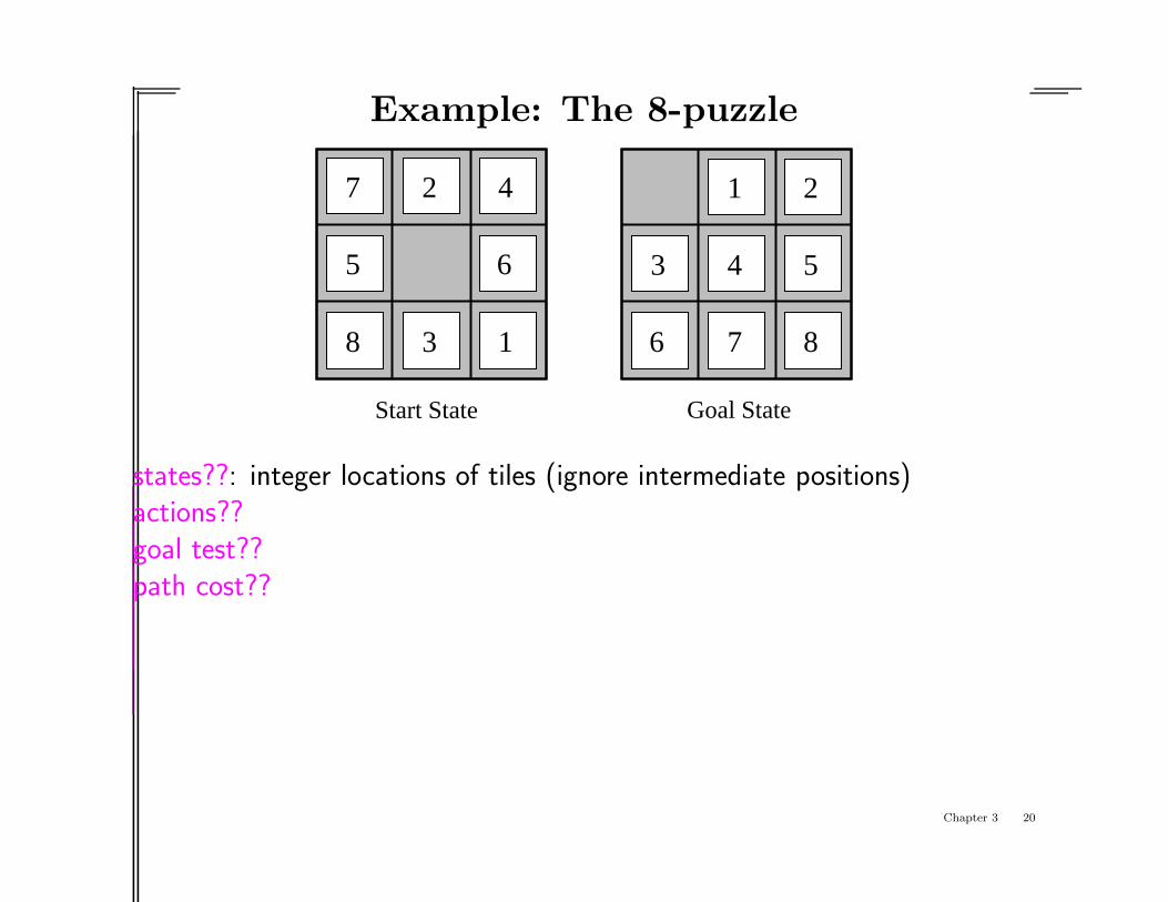
states??: integer locations of tiles (ignore intermediate positions)actions??goal test??path cost??
Chapter 3 20

Example: The 8-puzzle
2
Start State Goal State
1
3 4
6 7
5
1
2
3
4
6
7
8
5
8
states??: integer locations of tiles (ignore intermediate positions)actions??: move blank left, right, up, down (ignore unjamming etc.)goal test??path cost??
Chapter 3 21

Example: The 8-puzzle
2
Start State Goal State
1
3 4
6 7
5
1
2
3
4
6
7
8
5
8
states??: integer locations of tiles (ignore intermediate positions)actions??: move blank left, right, up, down (ignore unjamming etc.)goal test??: = goal state (given)path cost??
Chapter 3 22

Example: The 8-puzzle
2
Start State Goal State
1
3 4
6 7
5
1
2
3
4
6
7
8
5
8
states??: integer locations of tiles (ignore intermediate positions)actions??: move blank left, right, up, down (ignore unjamming etc.)goal test??: = goal state (given)path cost??: 1 per move
[Note: optimal solution of n-Puzzle family is NP-hard]
Chapter 3 23

Example: robotic assembly
R
RRP
R R
states??: real-valued coordinates of robot joint anglesand parts of the object to be assembled
actions??: continuous motions of robot joints
goal test??: complete assembly with no robot included!
path cost??: time to execute
Chapter 3 24
Tree search algorithms
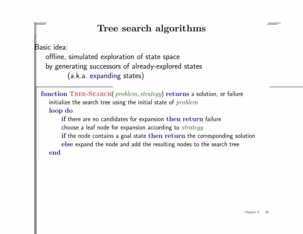
Basic idea:offline, simulated exploration of state spaceby generating successors of already-explored states
(a.k.a. expanding states)
function Tree-Search( problem, strategy) returns a solution, or failure
initialize the search tree using the initial state of problem
loop do
if there are no candidates for expansion then return failure
choose a leaf node for expansion according to strategy
if the node contains a goal state then return the corresponding solution
else expand the node and add the resulting nodes to the search tree
end
Chapter 3 25

Tree search example
Rimnicu Vilcea Lugoj
ZerindSibiu
Arad Fagaras Oradea
Timisoara
AradArad Oradea
Arad
Chapter 3 26

Tree search example
Rimnicu Vilcea LugojArad Fagaras Oradea AradArad Oradea
Zerind
Arad
Sibiu Timisoara
Chapter 3 27

Tree search example
Lugoj AradArad OradeaRimnicu Vilcea
Zerind
Arad
Sibiu
Arad Fagaras Oradea
Timisoara
Chapter 3 28
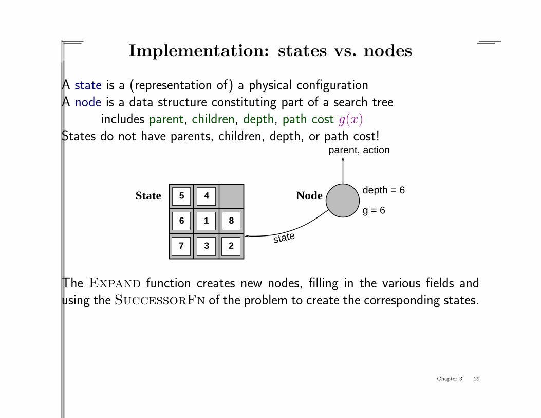
Implementation: states vs. nodes
A state is a (representation of) a physical configurationA node is a data structure constituting part of a search tree
includes parent, children, depth, path cost g(x)States do not have parents, children, depth, or path cost!
1
23
45
6
7
81
23
45
6
7
8
State Node depth = 6
g = 6
state
parent, action
The Expand function creates new nodes, filling in the various fields andusing the SuccessorFn of the problem to create the corresponding states.
Chapter 3 29

Implementation: general tree search
function Tree-Search( problem, fringe) returns a solution, or failure
fringe← Insert(Make-Node(Initial-State[problem]), fringe)
loop do
if fringe is empty then return failure
node←Remove-Front(fringe)
if Goal-Test(problem,State(node)) then return Solution(node)
fringe← InsertAll(Expand(node,problem), fringe)
function Expand(node, problem) returns a set of nodes
successors← the empty set; state←State[node]
for each action, result in Successor-Fn(problem, state) do
s← a new Node
Parent-Node[s]← node; Action[s]← action; State[s]← result
Path-Cost[s]←Path-Cost[node]+Step-Cost(state,action, result)
Depth[s]←Depth[node] + 1
add s to successors
return successors
Chapter 3 30

Search strategies
A strategy is defined by picking the order of node expansion
Strategies are evaluated along the following dimensions:completeness—does it always find a solution if one exists?time complexity—number of nodes generated/expandedspace complexity—maximum number of nodes in memoryoptimality—does it always find a least-cost solution?
Time and space complexity are measured in terms ofb—maximum branching factor of the search treed—depth of the least-cost solutionC∗—path cost of the least-cost solutionm—maximum depth of the state space (may be ∞)
Chapter 3 31
Uninformed search strategies
Uninformed strategies use only the information availablein the problem definition
Breadth-first search
Uniform-cost search
Depth-first search
Depth-limited search
Iterative deepening search
Chapter 3 32

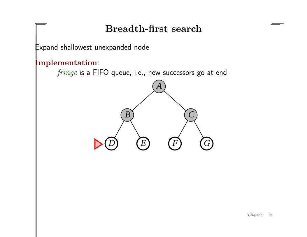
Breadth-first search
Expand shallowest unexpanded node
Implementation:fringe is a FIFO queue, i.e., new successors go at end
A
B C
D E F G
Chapter 3 33

Breadth-first search
Expand shallowest unexpanded node
Implementation:fringe is a FIFO queue, i.e., new successors go at end
A
B C
D E F G
Chapter 3 34

Breadth-first search
Expand shallowest unexpanded node
Implementation:fringe is a FIFO queue, i.e., new successors go at end
A
B C
D E F G
Chapter 3 35
Breadth-first search
Expand shallowest unexpanded node
Implementation:fringe is a FIFO queue, i.e., new successors go at end
A
B C
D E F G
Chapter 3 36

Properties of breadth-first search
Complete??
Chapter 3 37
Properties of breadth-first search
Complete?? Yes (if b is finite)
Time??
Chapter 3 38

Properties of breadth-first search
Complete?? Yes (if b is finite)
Time?? 1 + b + b2 + b3 + . . . + bd + b(bd − 1) = O(bd+1), i.e., exp. in d
Space??
Chapter 3 39

Properties of breadth-first search
Complete?? Yes (if b is finite)
Time?? 1 + b + b2 + b3 + . . . + bd + b(bd − 1) = O(bd+1), i.e., exp. in d
Space?? O(bd+1) (keeps every node in memory)
Optimal??
Chapter 3 40

Properties of breadth-first search
Complete?? Yes (if b is finite)
Time?? 1 + b + b2 + b3 + . . . + bd + b(bd − 1) = O(bd+1), i.e., exp. in d
Space?? O(bd+1) (keeps every node in memory)
Optimal?? No, unless step costs are constant
Space is the big problem; can easily generate nodes at 100MB/secso 24hrs = 8640GB.
Chapter 3 41

Uniform-cost search
Expand least-cost unexpanded node
Implementation:fringe = queue ordered by path cost, lowest first
Equivalent to breadth-first if step costs all equal
Complete?? Yes, if step cost ≥ ε
Time?? # of nodes with g ≤ cost of optimal solution, O(bdC∗/εe)
where C∗ is the cost of the optimal solution
Space?? # of nodes with g ≤ cost of optimal solution, O(bdC∗/εe)
Optimal?? Yes—nodes expanded in increasing order of g(n)
Chapter 3 42
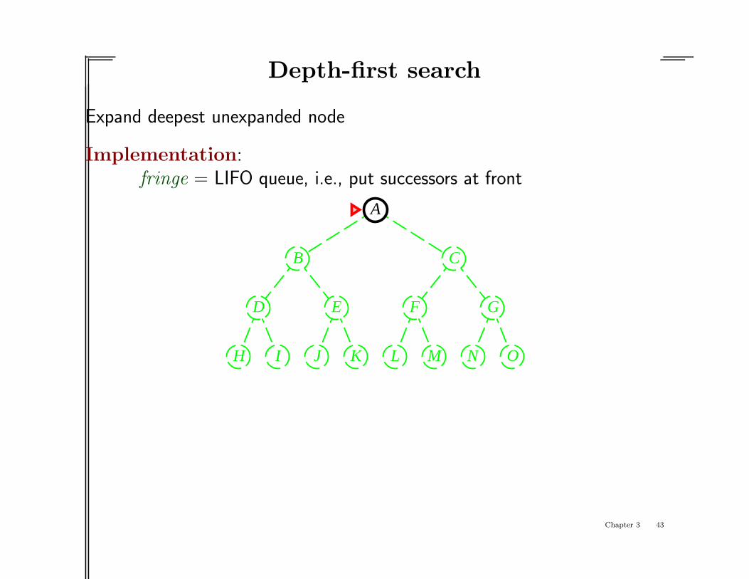
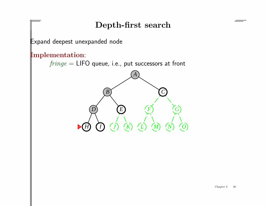
Depth-first search
Expand deepest unexpanded node
Implementation:fringe = LIFO queue, i.e., put successors at front
A
B C
D E F G
H I J K L M N O
Chapter 3 43

Depth-first search
Expand deepest unexpanded node
Implementation:fringe = LIFO queue, i.e., put successors at front
A
B C
D E F G
H I J K L M N O
Chapter 3 44

Depth-first search
Expand deepest unexpanded node
Implementation:fringe = LIFO queue, i.e., put successors at front
A
B C
D E F G
H I J K L M N O
Chapter 3 45
Depth-first search
Expand deepest unexpanded node
Implementation:fringe = LIFO queue, i.e., put successors at front
A
B C
D E F G
H I J K L M N O
Chapter 3 46

Depth-first search
Expand deepest unexpanded node
Implementation:fringe = LIFO queue, i.e., put successors at front
A
B C
D E F G
H I J K L M N O
Chapter 3 47

Depth-first search
Expand deepest unexpanded node
Implementation:fringe = LIFO queue, i.e., put successors at front
A
B C
D E F G
H I J K L M N O
Chapter 3 48

Depth-first search
Expand deepest unexpanded node
Implementation:fringe = LIFO queue, i.e., put successors at front
A
B C
D E F G
H I J K L M N O
Chapter 3 49

Depth-first search
Expand deepest unexpanded node
Implementation:fringe = LIFO queue, i.e., put successors at front
A
B C
D E F G
H I J K L M N O
Chapter 3 50

Depth-first search
Expand deepest unexpanded node
Implementation:fringe = LIFO queue, i.e., put successors at front
A
B C
D E F G
H I J K L M N O
Chapter 3 51

Depth-first search
Expand deepest unexpanded node
Implementation:fringe = LIFO queue, i.e., put successors at front
A
B C
D E F G
H I J K L M N O
Chapter 3 52

Depth-first search
Expand deepest unexpanded node
Implementation:fringe = LIFO queue, i.e., put successors at front
A
B C
D E F G
H I J K L M N O
Chapter 3 53

Depth-first search
Expand deepest unexpanded node
Implementation:fringe = LIFO queue, i.e., put successors at front
A
B C
D E F G
H I J K L M N O
Chapter 3 54
Properties of depth-first search
Complete??
Chapter 3 55

Properties of depth-first search
Complete?? No: fails in infinite-depth spaces, spaces with loopsModify to avoid repeated states along path⇒ complete in finite spaces
Time??
Chapter 3 56

Properties of depth-first search
Complete?? No: fails in infinite-depth spaces, spaces with loopsModify to avoid repeated states along path⇒ complete in finite spaces
Time?? O(bm): terrible if m is much larger than dbut if solutions are dense, may be much faster than breadth-first
Space??
Chapter 3 57

Properties of depth-first search
Complete?? No: fails in infinite-depth spaces, spaces with loopsModify to avoid repeated states along path⇒ complete in finite spaces
Time?? O(bm): terrible if m is much larger than dbut if solutions are dense, may be much faster than breadth-first
Space?? O(bm), i.e., linear space!
Optimal??
Chapter 3 58

Properties of depth-first search
Complete?? No: fails in infinite-depth spaces, spaces with loopsModify to avoid repeated states along path⇒ complete in finite spaces
Time?? O(bm): terrible if m is much larger than dbut if solutions are dense, may be much faster than breadth-first
Space?? O(bm), i.e., linear space!
Optimal?? No
Chapter 3 59

Depth-limited search
= depth-first search with depth limit l,returns cutoff if any path is cut off by depth limit
Recursive implementation:
function Depth-Limited-Search( problem, limit) returns soln/fail/cutoff
Recursive-DLS(Make-Node(Initial-State[problem]),problem, limit)
function Recursive-DLS(node,problem, limit) returns soln/fail/cutoff
cutoff-occurred?← false
if Goal-Test(problem,State[node]) then return node
else if Depth[node] = limit then return cutoff
else for each successor in Expand(node,problem) do
result←Recursive-DLS(successor,problem, limit)
if result = cutoff then cutoff-occurred?← true
else if result 6= failure then return result
if cutoff-occurred? then return cutoff else return failure
Chapter 3 60

Iterative deepening search
function Iterative-Deepening-Search( problem) returns a solution
inputs: problem, a problem
for depth← 0 to ∞ do
result←Depth-Limited-Search( problem, depth)
if result 6= cutoff then return result
end
Chapter 3 61

Iterative deepening search l = 0
Limit = 0 A A
Chapter 3 62

Iterative deepening search l = 1
Limit = 1 A
B C
A
B C
A
B C
A
B C
Chapter 3 63

Iterative deepening search l = 2
Limit = 2 A
B C
D E F G
A
B C
D E F G
A
B C
D E F G
A
B C
D E F G
A
B C
D E F G
A
B C
D E F G
A
B C
D E F G
A
B C
D E F G
Chapter 3 64

Iterative deepening search l = 3
Limit = 3
A
B C
D E F G
H I J K L M N O
A
B C
D E F G
H I J K L M N O
A
B C
D E F G
H I J K L M N O
A
B C
D E F G
H I J K L M N O
A
B C
D E F G
H I J K L M N O
A
B C
D E F G
H I J K L M N O
A
B C
D E F G
H I J K L M N O
A
B C
D E F G
H I J K L M N O
A
B C
D E F G
H I J K L M N O
A
B C
D E F G
H I J K L M N O
A
B C
D E F G
H J K L M N OI
A
B C
D E F G
H I J K L M N O
Chapter 3 65

Properties of iterative deepening search
Complete??
Chapter 3 66

Properties of iterative deepening search
Complete?? Yes
Time??
Chapter 3 67

Properties of iterative deepening search
Complete?? Yes
Time?? (d + 1)b0 + db1 + (d− 1)b2 + . . . + bd = O(bd)
Space??
Chapter 3 68

Properties of iterative deepening search
Complete?? Yes
Time?? (d + 1)b0 + db1 + (d− 1)b2 + . . . + bd = O(bd)
Space?? O(bd)
Optimal??
Chapter 3 69

Properties of iterative deepening search
Complete?? Yes
Time?? (d + 1)b0 + db1 + (d− 1)b2 + . . . + bd = O(bd)
Space?? O(bd)
Optimal?? No, unless step costs are constantCan be modified to explore uniform-cost tree
Numerical comparison for b = 10 and d = 5, solution at far right leaf:
N(IDS) = 50 + 400 + 3, 000 + 20, 000 + 100, 000 = 123, 450
N(BFS) = 10 + 100 + 1, 000 + 10, 000 + 100, 000 + 999, 990 = 1, 111, 100
IDS does better because other nodes at depth d are not expanded
BFS can be modified to apply goal test when a node is generated
Chapter 3 70
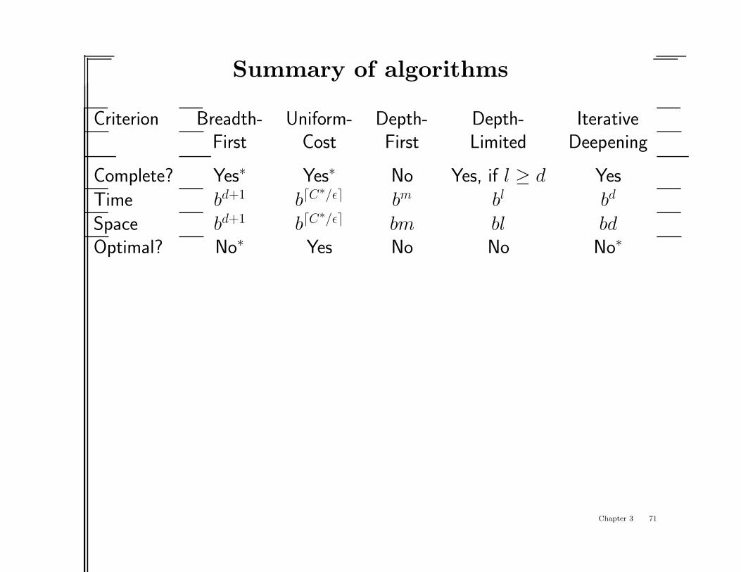
Summary of algorithms
Criterion Breadth- Uniform- Depth- Depth- IterativeFirst Cost First Limited Deepening
Complete? Yes∗ Yes∗ No Yes, if l ≥ d YesTime bd+1 bdC
∗/εe bm bl bd
Space bd+1 bdC∗/εe bm bl bd
Optimal? No∗ Yes No No No∗
Chapter 3 71

Repeated states
Failure to detect repeated states can cause exponentially more work!
A
B
C
D
A
BB
CCCC
Chapter 3 72
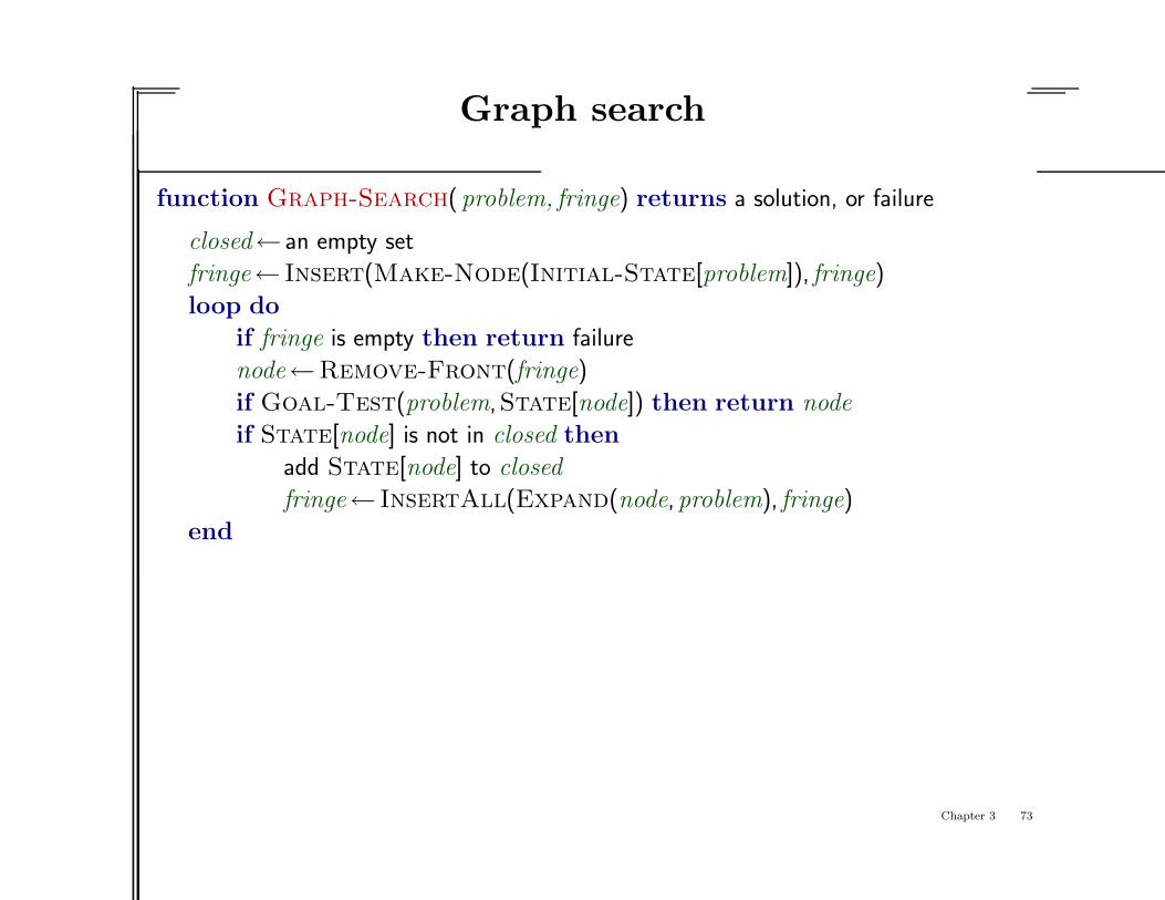
Graph search
function Graph-Search( problem, fringe) returns a solution, or failure
closed← an empty set
fringe← Insert(Make-Node(Initial-State[problem]), fringe)
loop do
if fringe is empty then return failure
node←Remove-Front(fringe)
if Goal-Test(problem,State[node]) then return node
if State[node] is not in closed then
add State[node] to closed
fringe← InsertAll(Expand(node,problem), fringe)
end
Chapter 3 73

Graph search
function Graph-Search( problem, fringe) returns a solution, or failure
closed← an empty set
fringe← Insert(Make-Node(Initial-State[problem]), fringe)
loop do
if fringe is empty then return failure
node←Remove-Front(fringe)
if Goal-Test(problem,State[node]) then return node
if State[node] is not in closed then
add State[node] to closed
fringe← InsertAll(Expand(node,problem), fringe)
end
Use hash table for closed — constant-time lookup!
Chapter 3 74

Graph search
function Graph-Search( problem, fringe) returns a solution, or failure
closed← an empty set
fringe← Insert(Make-Node(Initial-State[problem]), fringe)
loop do
if fringe is empty then return failure
node←Remove-Front(fringe)
if Goal-Test(problem,State[node]) then return node
if State[node] is not in closed then
add State[node] to closed
fringe← InsertAll(Expand(node,problem), fringe)
end
Use hash table for closed — constant-time lookup!Makes all algorithms complete in finite spaces!!
Chapter 3 75

Graph search
function Graph-Search( problem, fringe) returns a solution, or failure
closed← an empty set
fringe← Insert(Make-Node(Initial-State[problem]), fringe)
loop do
if fringe is empty then return failure
node←Remove-Front(fringe)
if Goal-Test(problem,State[node]) then return node
if State[node] is not in closed then
add State[node] to closed
fringe← InsertAll(Expand(node,problem), fringe)
end
Use hash table for closed — constant-time lookup!Makes all algorithms complete in finite spaces!!Makes all algorithms worst-case exponential space!!!
Chapter 3 76

Graph search
function Graph-Search( problem, fringe) returns a solution, or failure
closed← an empty set
fringe← Insert(Make-Node(Initial-State[problem]), fringe)
loop do
if fringe is empty then return failure
node←Remove-Front(fringe)
if Goal-Test(problem,State[node]) then return node
if State[node] is not in closed then
add State[node] to closed
fringe← InsertAll(Expand(node,problem), fringe)
end
Use hash table for closed — constant-time lookup!Makes all algorithms complete in finite spaces!!Makes all algorithms worst-case exponential space!!!But size of graph often much less than O(bd)!!!!
Chapter 3 77

Summary
Problem formulation usually requires abstracting away real-world details todefine a state space that can feasibly be explored
Variety of uninformed search strategies
Iterative deepening search uses only linear spaceand not much more time than other uninformed algorithms
Graph search can be exponentially more efficient than tree search
Chapter 3 78


![Bayes’ Nets [These slides were created by Dan Klein and Pieter Abbeel for CS188 Intro to AI at UC Berkeley. All CS188 materials are available at .]](https://static.fdocuments.net/doc/165x107/56649dc55503460f94ab8748/bayes-nets-these-slides-were-created-by-dan-klein-and-pieter-abbeel-for.jpg)