Chapter 3

Generalized Solutions of Bellman’s Differential Equa-tion

85

86 Chapter 3

3.0. Introduction

The theory of new distributions introduced in Chapter 1 can be used to definegeneralized solutions of the Hamilton–Jacobi–Bellman equation just as in theconventional linear theory, by using the adjoint operator. Idempotent analysisprovides a physically natural interpretation of formulas thus obtained: theyare given by the convolution (in the new sense) of the initial data with theGreen function (the solution whose initial value is given by the idempotent δ-function), which is obtained as the solution of the related variational problemwith fixed endpoints and fixed time interval.

This concept of generalized solutions originally arose from the analysisof the Burgers equation, which had earlier served as a starting point forHopf’s vanishing viscosity method. This example was considered in detailby V. P. Maslov in the book [?] and in the paper [?].

The first section of this chapter is introductory. We recall how first-orderequations arise in optimal control and discuss the problem of constructinggeneralized solutions. Section 2 mostly deals with the general conception ofweak (in the sense of idempotent analysis) solutions of evolution and station-ary Hamilton–Jacobi–Bellman equations. As was shown in [?], this theory,with minor modifications, can be extended to more general first-order partialdifferential equations. Similar constructions for quasilinear equations werecarried out in [?].

Since the differential Hamilton–Jacobi–Bellman equation is linear with re-spect to the operations ⊕ = min and ⊗ = +, we can look for linear finite-difference approximations to this equation. By writing out such an approxi-mation on analogy with a general pseudodifferential operator that is a differ-ence operator with respect to time, we obtain the general difference Bellmanequation. The following question is important: in what sense do the solu-tions of the difference Bellman equation converge to those of the differentialBellman equation? It turns out that weak convergence (studied in detail inChapter 1) takes place. We can use this fact in two ways: either solve thedifferential equation approximately with the aid of the difference equation,or obtain asymptotic formulas for solutions of discrete optimization problemswith a large parameter, solutions that assume finitely many values (say, 0 and1I) and hence should seemingly have no limit at all. However, the weak limitin the cited sense (the limit in idempotent measure of open sets) may wellexist. If we treat the discrete Bellman equation as an idempotent analog ofMarkov chains, then, on further analogy with probability theory, we can saythat the theory of generalized solutions of the differential Bellman equationallows one to prove limit theorems for idempotent measures. A result of thissort can be found in §3.9.

In §3.2 we also show that to each critical point of the Hamiltonian there cor-responds a generalized eigenfunction of the resolving operator of the Cauchyproblem for the corresponding differential Hamilton–Jacobi–Bellman equa-

Chapter 3 87

tion. Locally, this function is a generating function of the expanding La-grangian manifold of this point. As was already noted, the eigenfunctionsand eigenvalues of the Bellman operators determine the behavior of solutionsto optimization problems on the infinite planning horizon.

In the case of the differential Bellman equation, these eigenfunctions haveyet another application: they are limits as t → ∞ of logarithmic asymp-totics of solutions of tunnel-type equations. This matter is comprehensivelydiscussed in Chapter 4. The eigenfunctions of the resolving operator of theCauchy problem also specify generalized solutions of the stationary equation.Here we present a criterion for the semimodule of solutions of the stationaryBellman equation to be finite-dimensional and a theorem describing the limitbehavior of the Cauchy problem for large time.

The remaining sections of this chapter are independent from one anotherand develop the ideas of §3.2 in various directions.

Section 3.3 deals with the theory of stochastic perturbations of equationslinear in idempotent semimodules. These results, which were obtained in [?],are applied to quantum filtering methods of analysis of continuously observedquantum systems.

In §3.4 we derive and analyze a new differential Bellman type equation thatdescribes the dynamics of Pareto sets in multicriterial optimization problems.The exposition is based on the paper [?]. As a result, studying the dynamicsof Pareto sets in the general situation is reduced to solving a family of con-ventional optimization problems with a parameter. We give a simple exampleof how the proposed technique is applied to a variational problem with twoquadratic Lagrangians.

Generalized solutions of the first boundary value problem for the station-ary Hamilton–Jacobi equation H(x, ∂S/∂x) = 0 are considered in §3.5. Sys-tematic use of the idempotent superposition principle enables us to define anatural space (more precisely, an idempotent semimodule) in which the solu-tion of the considered problem exists and is unique. Our exposition in thissection follows [?]. Let us explain what this theory gives by considering a sim-ple example. Consider the equation (y′(x))2 = 1 on the interval [−1, 1] withthe boundary conditions y(−1) = y(1) = 0. It turns out that in an appropri-ately chosen semimodule of distributions corresponding to the arithmetic withthe operations ⊕ = min and ⊗ = +, this problem has the unique solutiony = 1− |x|. This is just the solution given by the vanishing viscosity method.On the other hand, if we start from the semimodules of distributions corre-sponding to the arithmetic with the operations ⊕ = max and ⊗ = +, thenthe unique solution of the problem in question is y = |x| − 1. Note also thatthe natural basis in the semimodule of solutions of the equation (y′(x))2 = 1on the interval [−1, 1] is formed by the functions y1 = x and y2 = −x andthat the cited solution of the boundary value problem is uniquely determinedas the linear combination y = a1⊗ y1⊕a2⊗ y2 of basis elements that satisfiesthe boundary conditions y(±1) = 0.

88 Chapter 3

The stochastic Hamilton–Jacobi–Bellman equation is considered in §3.6,and in §3.7 we deal with the turnpike theorem in general topological spaces andwith the limit theorem for the infinite-dimensional Hamilton-Jacobi equation.

Section 3.8 outlines the idempotent counterpart of calculus of variationsrecently constructed by M. D. Bronshtein and some of its applications toequations of mathematical physics.

In §3.9, Bellman’s differential equation is applied to studying discrete op-timization problems with a large parameter.

Yet another application of idempotent analysis to partial differential equa-tions can be found in [?].

3.1. First-Order Differential Equations in Calculus of Variations,Optimal Control, and Differential Games. The Problem of Con-structing Generalized Solutions

In this section, we recall how first-order differential equations (such as theHamilton–Jacobi, the Bellman, and the Isaacs equations) arise in calculusof variations, optimal control, and differential games. We also discuss thedifficulties encountered in constructing generalized solutions of the Cauchyproblem.

Let us start from calculus of variations. Let S(t, x, ξ) be the minimumof the functional

∫ t

0L(x, x) dt over all smooth curves x(τ) joining the points

ξ = x(0) and x = x(t); it is assumed that the function L(x, v), referred to asthe Lagrangian of the variational problem, is strictly convex with respect tov and smooth. Then for small t > 0 the Cauchy problem

∂S

∂t+ H

(x,

∂S

∂x

)= 0,

S|t=0 = S0(x)(3.1)

for the Hamilton–Jacobi equation with Hamiltonian function H that is theLegendre transform of L with respect to v (that is, H(x, p) = maxv(pv −L(x, v))) and with smooth initial function S0(x) has a unique solution S(t, x),which is given by the formula

S(t, x) = (RtS)(x) = minξ

(S(t, x, ξ) + S0(ξ)). (3.2)

In other words, the classical smooth solution of the Cauchy problem (3.1) isa solution of the variational minimization problem

∫ t

0

L(x, x) dt + S0(x(0)) → min (3.3)

with fixed time and free left endpoint. The two-point function S(t, x, ξ) itself

Chapter 3 89

can also be obtained from Eq. (3.2) by formally substituting the discontinuousfunction

δξ(x) =

0, x = ξ,+∞, x 6= ξ, (3.4)

(which is shown in Chapter 1 to be the idempotent analog of the usual δ-function) for S0(x).

Furthermore, it turns out that similar differential equations occur in solvingoptimal control problems; however, in contrast with the classical calculusof variations, the corresponding Hamiltonian is usually not smooth and theLagrangian L is discontinuous and assumes the value +∞ at some points. Forexample, consider the minimization problem (3.3) for a controlled object withdynamics described by the equation x = f(x, u), when u is a control parameterranging over a compact subset U in Euclidean space. Putting it other way, theminimum in (3.3) is sought not over all curves x(τ) with endpoint x = x(t),but only over the curves that satisfy the dynamic equations x = f(x, u(t)) forsome choice of the control u(t) ∈ U . In optimal control theory, such problemsare usually represented in the equivalent form

∫ t

0

g(x, u) dt + S0(x(0)) → min, (3.5)

where g(x, u) = L(x, f(x, u)). Obviously, problem (3.5) can also be repre-sented in the form

∫ t

0

L(x, x) dt + S0(x(0)) → min, (3.6)

obtained from (3.3) by replacing L with the discontinuous Lagrangian

L(x, x) =

L(x, x) if x = f(x, u) for some u ∈ U ,+∞ otherwise.

By formally applying the laws of the classical calculus of variations to thelatter Lagrangian, we can conclude that the minimum of S(t, x) in the optimalcontrol problem (3.5) or (3.6) is a (generalized, in some sense) solution of theCauchy problem

∂S

∂t+ H

(x,

∂S

∂x

)= 0,

S|t=0 = S0(x)(3.7)

for the Hamilton–Jacobi equation with nonsmooth Hamiltonian

H(x, p) = maxv

(pv − L(x, v)) = maxu∈U

(pf(x, u)− L(x, f(x, u))). (3.8)

90 Chapter 3

The equivalent form

∂S

∂t+ max

u∈U

(⟨∂S

∂t, f(x, u)

⟩− g(x, u)

)= 0 (3.9)

of the Hamiltonian–Jacobi equation with Hamiltonian H is called the nonsta-tionary Bellman differential equation.

Let us now recall how this equation can be obtained in optimal controltheory by Bellman’s dynamic programming method. Note, however, that thesubsequent calculations, though intuitively very natural, are in fact heuristic.They can be given precise meaning only for smooth solutions S(t, x) (or atleast in a neighborhood of smoothness points), whereas S is generally nons-mooth and even discontinuous if so is the initial condition S0.

By applying the optimality principle, according to which an optimal tra-jectory remains optimal after deleting an arbitrary initial segment, we canreadily obtain the approximate equation

S(t, x) = minu

(S(t−∆t, x−∆x(u)) + g(x, u)∆t). (3.10)

Let us expand S(t−∆t, x−∆x) in the Taylor series, neglect the terms of theorder of (∆t)2, and take into account the fact that ∆x = f(x, u)∆t in thisapproximation. Then we obtain

S(t, x) = minu

S(t, x)−∆t

(∂S

∂t(t, x)+

⟨f(x, u),

∂S

∂x(t, x)

⟩− g(x, u)

),

which is obviously equivalent to

minu

(− ∂S

∂t(t, x)−

⟨f(x, u),

∂S

∂x(t, x)

⟩+ g(x, u)

)= 0.

On replacing min by max and changing the sign, we obtain (3.9). Note that forthe case of a single terminal payment, when g(x, u) ≡ 0, Eq. (3.9) is reducedto the equation

∂S

∂t+ max

u

⟨∂S

∂x, f(x, u)

⟩= 0, (3.11)

whose Hamiltonian is first-order homogeneous with respect to the momenta.The above considerations suggest that the solutions of minimization prob-

lems in calculus of variations and optimal control theory are, in some sense,generalized solutions of the Cauchy problem for equations with nonsmoothHamiltonians. The initial functions can be nonsmooth and even discontin-uous. An example is given by the initial condition (3.4), satisfied by the

Chapter 3 91

two-point function S(t, x, ξ), which is a solution of the variational problemwith fixed endpoints. Discontinuous initial functions occur also in problemswhere the left endpoint x(0) must lie on some fixed submanifold M ⊂ Rn.For example, problem (3.3) with the additional condition x(0) ∈ M can berepresented in the form (3.3) with the cutoff initial function

S0 =

S0(x), x ∈ M ,+∞, x /∈ M .

A distinguishing feature of the Hamiltonians (3.8) occurring in calculus ofvariations and optimal control theory is that they are convex (possibly, non-strictly) in p; in particular, they are continuous in p. Hamiltonians of differentform occur in differential games. Let S(t, x0, y0) be the guaranteed approachin time t for an object P with dynamics x = f(x, u) pursuing an object Ewith dynamics y = g(y, v). Let u ∈ U and v ∈ V be the control parametersand x0, y0 ∈ R3 the initial states of the objects P and E, respectively. Just asabove, we apply the optimality principle and find that S(t, x, y) satisfies theHamilton–Jacobi equation

∂S

∂t+ max

u

⟨∂S

∂x, f(x, u)

⟩+ min

v

⟨∂S

∂y, g(y, v)

⟩= 0 (3.12)

with the initial condition S0(x, y) equal to the distance between x and y inR3. Equation (3.12) with the Hamiltonian

H(x, y, px, py) = maxu〈px, f(x, u)〉+ min

v〈py, g(y, v)〉 (3.13)

is known as the Isaacs equation in the theory of differential games. The Hamil-tonian (3.13), in contrast with (3.9) and (3.11), is convex-concave with respectto the momenta px and py. The theory of the Cauchy problem for equationswith convex-concave Hamiltonians (by the way, any Hamilton–Jacobi equa-tion, in a sense, can be reduced to such a problem) is much more complicatedthan the theory of the Cauchy problem for equations with convex Hamilto-nians and is not discussed in the present book. Some related results can befound in [?, ?, ?].

Stationary first-order equations of the form H(x, ∂S/∂x) = 0 play an im-portant role in optimal control theory. The simplest example is given by theclassical optimal time problem [?]: find a control u(t) such that the trajectoryof the equation x = f(x, u) issuing from a given point ξ reaches a given pointx in minimal time. Just as above, by applying the optimality principle, wecan show that the minimal time T (x) of transition from ξ to x satisfies thestationary equation

maxu〈T ′(x), f(x, u)〉 = 1 (3.14)

at every point where T (x) is smooth.

92 Chapter 3

Formally, the solution T (x) of the optimal time problem can be expressedvia the solution of the Cauchy problem for the nonstationary Hamilton–Jacobiequation with discontinuous initial data. Namely, let us define a functionS(t, x, ξ) as follows: S(t, x, ξ) = 0 if there exists a trajectory from ξ to x intime t, and S(t, x, ξ) = +∞ otherwise. Then S(t, x, ξ) is a generalized solutionof the Cauchy problem for Eq. (3.10) with the initial function (3.4). It readilyfollows from the definition of T (x) that

T (x) = inft≥0

(t + S(t, x, ξ)) (3.15)

Needless to say, to give precise meaning to the above heuristic considera-tions, one should correctly define the notion of a generalized solution of theCauchy problem for the Hamilton–Jacobi equation with nonsmooth Hamilto-nian convex with respect to the momenta and with discontinuous initial data;the definition should be independent of any optimization problems. Further-more, we must require the existence and uniqueness theorem to be valid forsuch a definition and the solution to be in some sense continuous with re-spect to the initial data. It is also desirable that for Hamiltonians of the form(3.9), which occur in optimal control theory, the solution thus defined be aminimum in the corresponding optimization problem and (in some sense) thelimit of solutions of the discrete Bellman equation (3.10). We now proceed todiscussing the definition and construction of such generalized solutions.

So, what difficulties occur when one tries to give a reasonable definition ofa solution? First, the classical (i.e., smooth) solution of the Cauchy problem(3.1) does not exist for large time even for smooth H and S0. This phe-nomenon is due to the fact that the characteristics, i.e., the projections onthe x-space of the solutions of Hamilton’s equations

x =∂H

∂p(x, p),

p = −∂H

∂x(x, p),

issuing from the points of the initial Lagrangian manifold p = ∂S0/∂x, mayintersect (e.g., see [?]). All the more, one cannot hope to obtain smoothsolutions for nonsmooth H and S0.

The obvious idea of defining a generalized solution, at least for continuousinitial data, as a continuous function that is smooth almost everywhere andsatisfies the equation at the differentiability points fails immediately, sincethere are infinitely many such solutions even for smooth H and S0. Indeed,consider the following simple example [?]. In the Cauchy problem

∂S

∂t+

12

(∂S

∂x

)2

= 0,

S|t=0 = S0(x)(3.16)

Chapter 3 93

for the Hamilton–Jacobi equation with Hamiltonian H(x, p) = 12p2, x, p ∈ R,

let us impose the zero initial data S0(x) = 0. It is easy to see that for eachδ > 0 the function

Sδ(t, x) =

0, |x| ≥ δt,δ|x| − 1

2δ2t, |x| ≤ δt,

is continuous and that outside the rays |x| = δt, t > 0, it is differentiable andsatisfies the equation ∂S/∂t + 1

2 (∂S/∂x)2 = 0.Finally, recall that, in contrast with the theory of linear equations, where

generalized solutions can be defined in the standard way as functionals on thespace of test functions, there is no such approach in the theory of nonlinearequations.

The most popular approach to the theory of generalized solutions of theHamilton–Jacobi equation is the vanishing viscosity method. For the firsttime, this method was applied by Hopf to the Cauchy problem (3.16). Hopfsuggested to define a generalized solution of problem (3.16) as the limit ash → 0 of the solution to the Cauchy problem for the parabolic equation

∂w

∂t+

12

(∂w

∂x

)2

− h

2∂2w

∂x2= 0 (3.17)

with small parameter h and with the same initial condition w0(x, h) = S0(x):S(t, x) = limh→0 w(t, x, h). Equation (3.17) is the integrated Burgers equa-tion. The substitution u = exp(−w/h) reduces Eq. (3.17) to the linear heatequation

∂u

∂t=

h

2∂2u

∂x2. (3.18)

The solution of Eq. (3.18) with the initial condition u0 = exp(−w0/h) is givenby the formula

u(t, x, h) =1√

2πht

∫exp

− (x− ξ)2

2th

u0(ξ) dξ.

The last expression readily implies the following formula for the solution ofthe Cauchy problem for Eq. (3.17):

w(t, x, h) = −h ln u(t, x, h)

= −h ln(

1√2πht

∫exp

− (x− ξ)2

2th− w0(ξ)

h

dξ

).

(3.19)

Thus, the definition of a generalized solution to the Cauchy problem (3.18)is reduced to calculating the logarithmic limit for the heat equation, which canreadily be performed by evaluating the asymptotics of the integral in (3.19)by the Laplace method.

94 Chapter 3

By extending this method to more general equations, we arrive at thedefinition of a generalized solution to problem (3.1) as the limit as h → 0 ofsolutions of the Cauchy problem

∂w

∂t+ H

(x,

∂w

∂x

)− h

2∂2w

∂x2= 0,

w|t=0 = w0(x) = S0(x).(3.20)

One cannot obtain a closed analytic expression for the solution w(t, x, h) ofthis problem. However, for continuous initial data and under some reason-able restrictions on the growth of H and S0, one can prove that there ex-ists a unique smooth solution w(t, x, h) of problem (3.20) and that the limitS(t, x) = limh→0 w(t, x, h) exists and is continuous. Furthermore, it turnsout that the solutions thus obtained are selected from the set of continuousfunctions satisfying the Hamilton–Jacobi equation almost everywhere by somesimple conditions on the discontinuities of the derivatives. In some cases, theseconditions have a natural physical interpretation. A detailed exposition of thevanishing viscosity method can be found in [?, ?, ?].

However, according to [?], this method cannot be used to construct a rea-sonable theory of generalized solutions of Eq. (3.1) for discontinuous initialfunctions. Furthermore, it is highly desirable to devise a theory of problems(3.1) on the basis of only intrinsic properties of Hamilton–Jacobi equations(i.e., regardless of the way in which the set of Hamilton–Jacobi equations isembedded in the set of higher-order equations). Such a theory, including so-lutions with discontinuous initial data, can be constructed for equations withconvex Hamiltonians on the basis of idempotent analysis; in fact, the set ofsolutions of such equations is equipped with an idempotent semigroup super-position law, and the theory of generalized solutions can be constructed byanalogy with linear equations, with the new superposition law replacing theusual one.

The form of this superposition law can be guessed easily from the simpleequation (3.16) and from Hopf’s method for solving this equation. Let usconsider the substitution w = −h ln u, which transforms the heat equationinto Eq. (3.16), as a semiring isomorphism. Obviously, this transformationtakes the semiring R+ (with standard addition and multiplication) to thesemiring Ah with the “sum”

a⊕ b = −h ln(exp(−a/h) + exp(−b/h)) (3.21)

and the “product”

a¯ λ = a + λ. (3.22)

The zero is taken to 0 = +∞ and the unity to 1I = 0; these are the neutralelements with respect to addition ⊕ and multiplication ¯ in the semiring Ah.

Chapter 3 95

The linear combination u = λ1u1 + λ2u2 of positive solutions to the heatequation with positive coefficients is taken to the “linear-combination”

w = − ln(

expµ1 − w1

h+ exp

µ2 − w2

h

)

of the solutions w1 and w2 to Eq. (3.17) in the semiring Ah; here µi = − ln λi,i = 1, 2. Obviously, this combination is also a solution of Eq. (3.17). Thus,we can say that Eq. (3.17) is linear with respect to the semiring operations⊕ and ¯. Let us equip the semimodule of Ah-valued functions with the innerproduct

〈w1, w2〉Ah= −h ln

∫exp

(− w1 + w2

h

)dx, (3.23)

which is obviously bilinear:

〈w1 ⊕ w2, w3〉Ah= 〈w1, w3〉Ah

⊕ 〈w2, w3〉Ah,

λ¯ 〈w1, w2〉Ah= 〈λ¯ w1, w2〉Ah

.(3.24)

Then the resolving operator Ltw0 (3.19) of the Cauchy problem for Eq. (3.17)is self-adjoint with respect to (3.23) (see the book [?] for detailed computa-tions).

The Burgers equation (3.17) passes as h → 0 into the Hamilton-Jacobiequation (3.16); the semiring Ah passes as h → 0 into the semiring A =R∪ +∞ with operations a⊕ b = min(a, b) and a¯ b = a + b. Furthermore,the inner product (3.23) passes into the inner product of A-valued functions,introduced in Chapter 1. Hence, it is natural to expect that the resolvingoperator of the Cauchy problem for the Hamilton-Jacobi equation is linearin the semimodule of A-valued functions, which was studied in Chapters 1and 2. This is the case indeed. More precisely, it turns out that the classicalresolving operator of problem (3.1) with convex Hamiltonian is defined andlinear with respect to the operations ⊕ = min and ¯ = + on the set of smoothconvex initial functions. Since (⊕,¯)-linear combinations of such functions aredense in the semimodule C∞0 (Rn), introduced in Chapter 2 (they approximateidempotent δ-functions) and since this semimodule is naturally embedded inthe dual semimodule with the help of the inner product

〈f, g〉A = infx

f(x)¯ g(x), (3.25)

it follows that the generalized solutions of (3.1) can naturally be defined asin the ususal linear theory, via the adjoint operator. This program is imple-mented in the next section.

Differentiation is known to reduce the Hamilton-Jacobi equation to a sys-tem of first-order quasilinear equations. The semimodule of continuous A-valued functions is then transformed into an interesting function semimodule,

96 Chapter 3

which is not a semimodule of semiring-valued functions and which can be usedto construct generalized solutions of quasilinear equations [?]. For example,let us discuss the situation for the (nonintegrated) Burgers equation.

Consider the space of pairs u(x), c, where u(x) is a function and c is aconstant. We introduce the operations

u1, c1 ⊕ u2, c2 =

hd

dxln

(exp

(1h

( ∫ x

0

u1(x) dx + c1

))

+exp(

1h

( ∫ x

0

u2(x) dx + c2

))), h ln

(exp

c1

h+ exp

c2

h

),

u1, c1 ¯ λ = u1, c1 + λ,u1, c1 ¯ u2, c2 = u1 + u2, c1 + c2,

the involution

u, c∗ = −u,−c,and the “inner product” given by the bilinear form

(u1, c1∗, u2, c2) =

= ln∫

exp(

1h

( ∫ x

0

(u1(x)− u2(x)) dx + (c2 − c1)))

dx.

The (matrix) resolving operator for the pair of equations

∂u

∂t+ u

∂u

∂x=

h

2∂2u

∂x2,

∂c

∂t=

h

2∂u

∂xux(0, t)− 1

2u2(0, t)

is linear in the described space, eqipped with the structure of a module. Notethat one of these equations is the Burgers equation itself. We see that thesituation, though more complicated, is essentially the same.

In closing, note that formulas (3.2) and (3.15) for the solution of theHamilton-Jacobi equation have quite a natural interpretation in idempotentanalysis. The function S(t, x, ξ) in (3.2), which is a solution of the Cauchyproblem with the initial data given by the idempotent δ-function (3.4), is ananalog of the Green function in the theory of linear partial differential equa-tions. Equation (3.2), which can be rewritten via the idempotent integral inthe form

S(t, x) =∫ ⊕

Rn

S(t, x, ξ)¯ S0(ξ) dξ,

is an analog of the Green function representation of the solution to a linearCauchy problem, and Eq. (3.15), rewritten in the equivalent form

T (x) =∫ ⊕

t≤0

t¯ S(t, x, ξ) dµ(t),

Chapter 3 97

is a linear formula that expresses the stationary solution via the Green func-tion S(t, x, ξ).

3.2. Generalized Solutions of the Hamilton–Jacobi–Bellman Equa-tion and Eigenfunctions of the Resolving Operator of the CauchyProblem

For simplicity, we first consider equations that do not depend on the argu-ment x explicitly. We begin with constructing a supply of classical (smooth)solutions by the method of generalized (subgradient) characteristics.

Consider the Cauchy problem

∂S

∂t+ H

(∂S

∂x

)= 0,

S|t=0 = S0(x),(3.26)

where x ∈ Rn and H:Rn → R is a convex function (we do not require H to bestrictly convex). Note that H is continuous, which follows from the fact thatit is finite and convex, but no additional smoothness conditions are imposed.Let us also note that in control theory H is usually represented in the form

H(p) = max(f,g)∈F

(〈f, p〉+ g), (3.27)

where F is some compact set in Rn+1.Let L(v) be the Legendre transform of H(p). Then L is also convex, but

it can be discontinuous and assume the value +∞. Let us define an operatorfamily Rtt>0 acting on functions S0(x) bounded below by setting

(RtS0)(x) = S(t, x) = infξ∈Rn

(S0(ξ) + tL

(x− ξ

t

)). (3.28)

The operators Rt are obviously linear with respect to the operations ⊕ = minand ¯ = + and are characterized by the property that their kernels (see §3.1)are convex functions of the difference of the arguments.

Proposition 3.1 ([?]) Let S0(x) be smooth and strongly convex, so that forall x the eigenvalues of the Hessian matrix S′′0 (x) are not less than some δ > 0.Then

1) For any x ∈ Rn and t > 0 there exists a unique ξ(t, x) ∈ Rn such that(x− ξ(t, x))/t is a subgradient of H at the point S′0(ξ(t, x)); moreover,

(RtS0)(x) = S0(ξ(t, x)) + tL

(x− ξ(t, x)

t

). (3.29)

2) For t > 0 the mapping ξ(t, x) is Lipschitz continuous on compact sets,and limt→0 ξ(t, x) = x.

98 Chapter 3

3) The Cauchy problem (3.26) has a unique C1 solution. This solution isgiven by Eq. (3.28) or Eq. (3.29) and satisfies

∂S

∂x(t, x) = S′0(ξ(t, x)).

Remark 3.1 If H is a homogeneous function of the form (3.27), thenEq. (3.29) acquires the especially simple form

RtS0(x) = minS0(ξ) : ξ ∈ x− t coF,where coF is the convex hull of a set F .Remark 3.2 Proposition 3.1 is quite obvious if H is smooth and strictlyconvex, since in this case L is also smooth and all subgradients involved areusual gradients.

We postpone the proof of Proposition 3.1, which is rather lengthy andtechnical, until stating Theorem 3.1 so as not to interrupt the exposition.

As was noted in Chapter 2, smooth convex functions form a “complete”subset in C∞0 (R2n), since they approximate the “δ-function”

δξ(x) = limn→∞

n(x− ξ)2 =

1I = 0, x = ξ,0 = +∞, x 6= ξ.

Consequently, each functional ϕ ∈ (C∞0 (Rn))∗ is uniquely determined by itsvalues on this set of functions.

The Cauchy problem

∂S

∂t+ H

(− ∂S

∂x

)= 0,

S|t=0 = S0(x)(3.30)

with Hamiltonian H(p) = H(−p) will be called the adjoint problem of theCauchy problem (3.26). Obviously, the classical resolving operator R∗t of theCauchy problem (3.29), which is determined on smooth convex functions bythe formula

(R∗t S0)(x) = infξ

(S0(ξ) + tL

(ξ − x

t

)), (3.31)

is linear (with respect to the operations ⊕ = min and ¯ = +) on this setof functions and is the adjoint of the resolving operator Rt of the Cauchyproblem (3.26) with respect to the inner product introduced in §1.2. We arenow in a position to define weak solutions of problem (3.26) by analogy withthe theory of linear equations; we also take into account the fact that, byTheorem 2.1.2, the functionals ϕ ∈ (C∞0 (Rn))∗ are given by usual functionsbounded below.Definition 3.1 Let S0:Rn → A = R ∪ +∞ be a function bounded below,and let mS0 ∈ (C∞0 (Rn))∗ be the corresponding functional. The generalized

Chapter 3 99

weak solution of the Cauchy problem (3.26) is the function (RtS0)(x) deter-mined by the equation

mRtS0(ψ) = mS0(R∗t ψ)

for all smooth strictly convex functions ψ.The following theorem is a direct consequence of Definition 3.1, Theorem

2.2, and Proposition 3.1.

Theorem 3.1 For an arbitrary function S0(x) bounded below, the generalizedweak solution of the Cauchy problem (3.26) exists and can be found accordingto the formula

(RtS0)(x) = infξ

(S0(ξ) + tL

(x− ξ

t

)).

Various solutions have the same lower semicontinuous closure Cl, so the so-lution in the class of semicontinuous functions is unique and is given by theformula

Cl(RtS0) = Rt Cl S0.

Proof of Proposition 3.1. 1) Let us prove the uniqueness of a point ξ(t, x) withthe desired property. We use the following general inequality, which readilyfollows from the definition of a subgradient [?]: if α1 and α2 are subgradientsof F (u) at points u1 and u2, respectively, then

〈α1 − α2, u1 − u2〉 ≥ 0,

and the inequality is strict if F (u) is strictly convex.Suppose that there exist two points ξ1 6= ξ2 such that αi = (x − ξi)/t are

subgradients of H at S′0(ξi), i = 1, 2. Then

x = ξ1 + tα1 = ξ2 + tα2.

By the cited inequality,

〈(ξ1 + tα1)− (ξ2 + tα2), S′0(ξ1)− S′0(ξ2)〉= 〈ξ1 − ξ2, S

′0(ξ1)− S′0(ξ2)〉+ t〈α1 − α2, S

′0(ξ1)− S′0(ξ2)〉 > 0.

This contradiction proves that ξ(t, x) is unique.To prove the existence of ξ(t, x) and Eq. (3.29), let us show that if ξ(t, x) is

the point at which the infimum in Eq. (3.28) is attained (this point exists andis unique since S0(x) is strongly convex), then (x− ξ(t, x))/t is a subgradientof H at S′0(ξ).

The point ξ = ξ(t, x) of infimum in Eq. (3.28) can be characterized by thevariational inequality [?]

〈S′0(ξ), η − ξ〉+ tL

(x− η

t

)− tL

(x− ξ

t

)≥ 0 ∀η. (3.32)

100 Chapter 3

We write

ψ(ξ) =x− ξ

t, ϕ =

x− η

t

and find that inequality (3.32) is equivalent to the inequality

〈S′0(ξ), ψ(ξ)− ϕ〉+ L(ϕ)− L(ψ(ξ)) ≥ 0,

or

〈S′0(ξ), ψ(ξ)〉 − L(ψ(ξ)) ≥ 〈S′0(ξ), ϕ〉 − L(ϕ),

for all ϕ. Since H is the Legendre transform of L, it follows from the lastinequality that its left-hand side is equal to H(S′0(ξ)), that is,

H(S′0(ξ)) + L(ψ(ξ)) = 〈S′0(ξ), ψ(ξ)〉. (3.33)

The last equation is characteristic of the subgradient [?], whence it followsthat ψ(ξ) = (x− ξ)/t is a subgradient of H at S′0(ξ), as desired.

2) By using the variational inequalities (3.32) at the points ξ = ξ(t, x) andη = ξ(τ, y), we obtain

⟨S′0(ξ),

x− ξ

t− y − η

τ

⟩+ L

(y − η

τ

)− L

(x− ξ

t

)≥ 0,

⟨S′0(η),

y − η

τ− x− ξ

t

⟩+ L

(x− ξ

t

)− L

(y − η

τ

)≥ 0.

Adding these inequalities yields

〈S′0(ξ)− S′0(η), τx− ty〉 ≥ 〈S′0(ξ)− S′0(η), τξ − tη〉, (3.34)

or

〈S′0(ξ)− S′0(η), τ(x− y) + (τ − t)(y− η)〉 ≥ τ〈S′0(ξ)− S′0(η), ξ − η〉.(3.35)

It is easy to see that if (x, t) and (y, t) belong to some compact subset P of thedomain t > 0, then ξ and η also lie in some compact set (this was provedin the beginning of item 3). Hence, by using the inequalities

〈S′0(ξ)− S′0(η), ξ − η〉 ≥ δ‖ξ − η‖2,‖S′0(ξ)− S′0(η)‖ ≤ 2‖ξ − η‖ max

θ∈[ξ,η]‖S′′0 (θ)‖,

from Eq. (3.33) we obtain

δ‖ξ − η‖2τ ≤ 2λ(τ‖x− y‖+ (τ − t)‖y − η‖)‖ξ − η‖,for t > τ , where λ is some constant depending on P . It follows that ξ(t, x) isLipschitz continuous on compact subsets in t > 0.

Chapter 3 101

Obviously, ‖ξ(t, x)‖ is bounded if x is fixed and t ≤ t0. Hence, shouldξ(t, x) → y 6= x as t → 0 along some sequence, the norm of the subgradient(x − ξ(t, x))/t along the same sequence would tend to infinity, which is im-possible since the set of subgradients of H(p) in each compact neighborhoodof S′0(y) is bounded. We conclude that ξ(t, x) → x as t → 0.

3) a) By (3.33), Eq. (3.29) can be rewritten in the form

S(t, x) = S0(ξ) + 〈S′0(ξ), x− ξ〉 − tH(S′0(ξ)),

where ξ = ξ(t, x). It follows, in view of 2), that S(t, x) is continuous and theinitial conditions are satisfied.

b) Clearly, L(v) → +∞ as ‖v‖ → +∞, since

L(v) ≥ max‖p‖=1

(pv −H(p)).

Hence, there exists an A > 0 such that L(v) > L(0) whenever ‖v‖ ≥ A.Let P be a compact set in the half-space x ∈ Rn, t > 0. Then there

exists a compact set K ⊂ Rn such that for ξ 6= K and (t, x) ∈ P we haveS0(ξ) > S0(x), ‖(x− ξ)/t‖ ≥ A, and hence,

S0(ξ) + tL

(x− ξ

t

)> S0(x) + tL(0).

It follows that if (t, x) ∈ P , then ξ(t, x) ∈ K, and consequently,

S(t, x) = minξ∈K

(S0(ξ) + tL

(x− ξ

t

)).

c) Let us now take some B > A such that the ball

QB = v : ‖v‖ ≤ Bcontains the set

v = (x− ξ)/t : (t, x) ∈ P, ξ ∈ Kand construct a sequence of smooth strictly convex functions Ln:Rn → R sothat in QB this sequence is monotone increasing and pointwise convergent toL. Such a sequence can be constructed, say, by smoothing (integral averagingof) the sequence

Ln(v) = max‖p‖≤n

(pv −H(p)),

which consists of continuous convex everywhere finite functions and is point-wise monotonically convergent to L. By discarding a few first terms wherenecessary, we can assume that L1(v) > L(0) for ‖v‖ = A, and hence, Ln(v) >Ln(0) for all n for ‖v‖ = A.

102 Chapter 3

Let Hn be the Legendre transform of Ln. Then Hn is smooth and strictlyconvex, and so the statement of Lemma 3.1 is trivial for the correspondingCauchy problem

∂S

∂t+ Hn

(∂S

∂x

)= 0,

S|t=0 = S0(x).(3.36)

Let ξn(t, x) denote the mapping associated with Hn by virtue of item 1) ofthis lemma. Then the formula

Sn(t, x) = S0(ξn(t, x)) + Ln

(x− ξn(t, x)

t

)

specifies a smooth solution of the Cauchy problem (3.36), and

∂Sn

∂x(t, x) = S′0(ξn(t, x)).

By virtue of the cited assumptions, ξn(t, x) ∈ K for any n whenever (t, x) ∈ P .Hence,

Sn(t, x) = minξ∈K

(S0(ξ) + tLn

(x− ξ

t

)).

Thus, for (t, x) ∈ P the sequence Sn(t, x) of smooth functions is monotonenondecreasing as n → ∞ and is bounded above by S(t, x). We see that thissequence has a limit

S(t, x) = limn→∞

Sn(t, x) ≤ S(t, x)

for (t, x) ∈ P .d) Let (t, x) ∈ P . Let us prove that

ξn = ξn(t, x) → ξ = ξ(t, x)

as n → ∞ and that S(t, x) = S(t, x). Consider an arbitrary subsequenceof ξn convergent to a point η0 ∈ K. The assumption L((x − η0)/t) = +∞immediately results in a contradiction, and so in what follows we assume thatL((x − η0)/t) is finite. Then for any ε > 0 there exists a positive integer Nsuch that

Ln

(x− η

t

)> L

(x− η

t

)− ε (3.37)

for n > 0. Then inequality (3.37) obviously holds for all η in some neighbor-hood of η0. Hence,

Sn(t, x) = S0(ξn) + tLn

(x− ξn

t

)> S0(ξn) + t

(L

(x− η0

t

)− ε

)

Chapter 3 103

for large n. Since ε is arbitrary, by passing to the limit we obtain

S(t, x) ≥ S0(η0) + tL

(x− η0

t

)≥ S(t, x),

whence it follows that S(t, x) = S(t, x) and η0 = ξ.e) Since the sequence Sn is monotone and the functions Sn and S are

continuous, it follows that the convergence Sn → S is uniform on the compactset P . Hence, so is the convergence ξn → ξ; indeed,

|S(t, x)− Sn(t, x)| = S(t, x)− Sn(t, x)

= S0(ξ) + L

(x− ξ

t

)− S0(ξn)− Ln

(x− ξn

t

)

− Ln

(x− ξ

t

)+ Ln

(x− ξ

t

)

≥(

S0(ξ) + Ln

(x− ξ

t

))−

(S0(ξn) + Ln

(x− ξn

t

))≥ δ

2‖ξ − ξn‖2.

f) Thus, the smooth functions Sn(t, x) are uniformly convergent to S(t, x)on P , and their derivatives

∂Sn

∂x(t, x) = S′0(ξn(t, x))

and

∂Sn

∂t= −Hn(S′0(ξn(t, x))) = Ln

(x− ξn

t

)−

⟨S′0(ξn),

x− ξn

t

⟩

=1t

[Sn(t, x)− S0(ξn)− 〈S′0(ξn), x− ξn〉]

are uniformly convergent to the functions S′0(ξ(t, x)) and −H(S′0(ξ(t, x))), re-spectively, by virtue of e). It follows that the latter functions are the deriva-tives of S(t, x), and so S(t, x) is a C1 solution of the Cauchy problem (3.26).

g) The uniqueness of a smooth solution is a standard consequence of thefact that H(p) is locally Lipschitz continuous.

Proposition 3.1 is proved.Let us now proceed to the Cauchy problem

∂S

∂t+ H

(x,

∂S

∂x

)= 0,

S|t=0 = S0(x)(3.38)

with general Hamiltonian H convex in p. We define generalized solutionsfor the case of a smooth function H by analogy with problem (3.26); fornonsmooth H, a limit procedure will be applied.

104 Chapter 3

Let H satisfy the following conditions.1) H is C2.2) The second derivatives of H are uniformly bounded:

max(

supx,p

∥∥∥∥∂2H

∂x2

∥∥∥∥, supx,p

∥∥∥∥∂2H

∂x∂p

∥∥∥∥, supx,p

∥∥∥∥∂2H

∂p2

∥∥∥∥)≤ c = const .

3) H is strongly convex; that is, there exists a constant δ > 0 such thatthe least eigenvalue of the matrix ∂2H/∂p2 is greater than or equal to δ forall (x, p).

By (y(τ, ξ, p0), p(τ, ξ, p0)) we denote the solution of Hamilton’s system

y =∂H

∂p,

p = −∂H

∂x

(3.39)

with the initial conditions y(0) = ξ, p(0) = p0. It follows from theory ofordinary differential equations that under the stated conditions the solutionexists and is unique for all t ≥ 0 and for any (ξ, p0). Let S(t, x, ξ) denote thegreatest lower bound of the action functional

∫ t

0

L(z(τ), z(τ)) dτ (3.40)

over all continuous piecewise smooth curves joining ξ with x in time t (z(0) = ξand z(t) = x). Here L(x, v) is the Lagrangian of the variational problemassociated with H, that is, the Legendre transform of H with respect to thevariable p.

The following assertion comprises some useful facts from calculus of varia-tions.

Proposition 3.2 Let H satisfy the above-stated conditions. Thena) The derivatives of the solution of system (3.36) with respect to the initial

data are given by the formulas

∂y

∂p0=

∫ t

0

∂2H

∂p2(y(τ), p(τ)) dτ + O(t2),

∂p

∂p0= E + O(t),

(3.41)

where E is the identity matrix and the estimates O(t) and O(t2) are uniformwith respect to ξ, p0, and t ∈ [0, t0] for each fixed t0.

b) There exists a t0 > 0 such that for any t ≤ t0, ξ, and x the equationy(t, ξ, p0) = x has a unique solution p0 = p0(t, x, ξ). This solution provides

Chapter 3 105

minimum in the corresponding variational problem with fixed endpoints, thatis,

S(t, x, ξ) =∫ t

0

L(y(τ), y(τ)) dτ,

where y(τ) = y(τ, ξ, p0(t, x, ξ)).c) For t ≤ t0, the function S(t, x, ξ) defined in b) is twice continuously

differentiable and strictly convex both in ξ and in x.

Scheme of the proof. Equations (3.41) can be obtained by analyzing thevariational system along the solutions of system (3.39). Let us prove b). Itfollows from Eq. (3.41) that

∂y

∂p0= tY (t) + O(t2),

where the matrix Y (t) is a smooth function of t, p0, and ξ for t > 0, issymmetric, and has eigenvalues that all lie in the interval [δ, c]. It follows thatthe matrix ∂y/∂p0 is invertible for t ≤ t0 for some fixed t0. Then, by theinverse function theorem, for any fixed t ≤ t0 and ξ ∈ Rn the mapping

P :Rn → Rn, p0 7→ y(t, ξ, p0)

is locally invertible in a neighborhood of each p0 ∈ Rn; moreover, P (p0) →∞as p0 → ∞. We see that the range of P is open and closed in Rn andhence coincides with Rn, so that P :Rn → Rn is surjective. Consequently, Pis a covering and, what is more, the universal covering, since Rn is simplyconnected. It follows from the properties of universal coverings that P isa bijection. Indeed, the preimage of each point (the fiber of the universalcovering) is an orbit of the monodromy group, which is isomorphic to thefundamental group of the space Rn (the base of the covering) and hence trivial.Thus, we have proved that for any x and ξ there exists a unique p0 such thaty(t, ξ, p0) = x. The fact that this solution provides a minimum of the actionfunctional follows from the standard criteria in calculus of variations. Indeed,the extremal y(τ) can be included in a field of extremals and the LagrangianL is convex in the second argument. Item c) now follows from the well-knownformula

∂2S

∂x2(t, x, ξ) =

∂p(t, ξ, p0(t, x, x))∂x

=∂p

∂p0

(∂y

∂p0

)−1

(3.42)

for the derivatives of S. By Proposition 3.2, if the initial function S0(x) inthe Cauchy problem (3.38) is convex, then the function

(RtS0)(x) = S(t, x) = minξ

(S0(ξ) + S(t, x, ξ)) (3.43)

106 Chapter 3

is continuously differentiable for all t ≤ t0 and x ∈ Rn. Indeed, the minimumin (3.43) is obviously attained at a unique point ξ(t, x). Therefore, Eq. (3.43)specifies the unique classical solution of the Cauchy problem (3.38). Thus, thetechnique of determining the usual solutions of the Cauchy problem (3.38) fort ≤ t0 for an arbitrary initial function S0(x) via the resolving operator of theadjoint Cauchy problem

∂S

∂t+ H

(x,−∂S

∂x

)= 0,

S|t=0 = S0(x)(3.44)

is just a reproduction of the method presented above for Hamiltonians inde-pendent of x. For t ≥ t0, the resolving operator (3.38) is defined via iterationsof the resolving operator given for t ≤ t0. As a result, we conclude that thefollowing assertion is valid.

Theorem 3.2 Suppose that the Hamiltonian H satisfies the above-stated con-ditions. Then for any function S(x) bounded below the Cauchy problem (3.35)is solvable and the solution is unique modulo functions with the same lowersemicontinuous closure. The solution is equal to Rt Cl S0 = Cl RtS0, where

(RtS0)(x) = infξ

(S0(ξ) + S(t, x, ξ)). (3.45)

Furthermore, it is obvious that if a smooth function of the form S(t, x) =S0(x) + tλ is a solution of problem (3.38), then S0(x) is a classical solution ofthe stationary equation

H

(x,

∂S

∂x

)+ λ = 0. (3.46)

Thus, it is natural to define a generalized solution of Eq. (3.46) as an eigen-function (in the sense of idempotent analysis) of the resolving operator (3.45)of the nonstationary problem. Let the Lagrangian L(x, v), defined as theLegendre transform of H(x, p) with respect to p, satisfy L(x, v) → ∞ as‖x‖, ‖v‖ → ∞. Then the operator Rt (3.45) is a compact A-linear operatorand has at most one eigenvalue by Theorem 2.3.2. It turns out that in thiscase there is a natural method of constructing eigenfunctions of Rt (gener-alized solutions of Eq. (3.46)). We consider the important particular case inwhich the semimodule of generalized solutions is finite-dimensional. This isjust the situation occurring when multiplicative asymptotics are studied inChapter 4.

Theorem 3.3 ([?]) Suppose that L(x, v) has finitely many points of mini-mum (ξ1, 0), . . . , (ξk, 0). Then λ = minx,v L(x, v) is a value for which thereexist generalized solutions of the stationary problem (3.46); the semimodule

Chapter 3 107

of these solutions (in the sense of idempotent structure) has a finite basisS1, . . . , Sk, where Sj(x) is the infimum of the functional

Jj(q( · )) =∫ t

0

(L(q(τ), q(τ))− λ) dt (3.47)

over all t > 0 and all piecewise smooth curves joining ξj with x in time t.Moreover, the operator family Rt − λt converges as t → 0 to the finite-dimensional operator B given by the formula

(Bh)(x) =⊕

j

〈h, Sj〉A ¯ Sj(x), (3.48)

where S1, . . . , Sk is a basis of the eigensemimodule for the adjoint operator.

Proof. Let us show that each Sj is an eigenfunction of the resolving operator(3.18):

(RtSj)(x) = infξ

infτ≥0

(S(τ, ξ, ξj)− τλ + S(t, x, ξ))

= infτ≥0

(S(t + τ, x, ξj)− τλ) = infτ≥t

(S(τ, x, ξj)− τλ + tλ)

= infτ≥0

(S(τ, x, ξj) + τλ) + tλ = Sj(x) + λt.

The limit equation (3.48) means that the family Rt − λt is convergent to theoperator with the decomposable kernel

k⊕

j=1

Sj(x)¯ Sj(y),

which can be proved by analogy with Theorem 2.3.4.Let us return to the general Cauchy problem (3.35). Suppose that the

Hamiltonian H is representable as the limit (uniform on compact sets) of asequence of Hamiltonians Hn satisfying the assumptions of Theorem 3.2. Itis clear that if we define generalized solutions of problem (3.35) as the limitsof the corresponding solutions of the Cauchy problems with HamiltoniansHn, then Theorem 3.2 will be valid for H. In optimal control theory, theHamiltonians H(x, p) homogeneous in p, namely, those given by the formula

H(x, p) = maxu∈U

〈f(x, u), p〉, (3.49)

are of special importance, where U is a compact set and f(x, u) is a functioncontinuous on Rn × U and Lipschitz continuous in x uniformly with respectto u ∈ U :

|f(x1, u)− f(x2, u)| ≤ L‖x1 − x2‖

108 Chapter 3

for any x1, x2 ∈ Rn, any u ∈ U , and some L. As was indicated in §3.1, prob-lems with Hamiltonians of this sort arise when dynamic programming is usedto find optimal trajectories of controlled objects whose motion is describedby the law x = f(x, u). For homogeneous Hamiltonians, Eq. (3.43) can berewritten in the special form

(RtS0)(x) = infS0(ξ) : ξ ∈ K(t, x), (3.50)

where K(t, x) is the t-slice of the integral funnel of the generalized differentialequation y ∈ −F (y), issuing from x at t = 0. Here F (y) is the convex hull ofthe compact set f(y, u) : u ∈ U. This formula follows from Eq. (3.43) andfrom the fact that the Legendre transform of the function H (3.49) has theform

L(x, v) =

0, v ∈ F (x),+∞, v /∈ F (x),

so that the action functional (3.38) in this situation is equal to zero on thesolutions of the generalized differential equation x ∈ F (x) and is infinite onany other trajectory. Equation (3.50) can also be obtained directly with theaid of the adjoint operator, as in Theorem 3.1 (see [?]).

The differential Bellman equation is formally obtained by passing to thelimit in the discrete Bellman equation (cf. §3.1). We can ascribe exact meaningto this passage to the limit by using the cited notion of a generalized solutionand linearity.

Let us define an operator ∆τ on functions ϕ(x) bounded below by theformula

(∆τϕ)(x) = infu

ϕ(x− f(x, u)τ).

For each initial function S0(x) of this class, we consider the sequence of func-tions

Sk(t, x) = (∆kτS0)(x), τ = t/k. (3.51)

Lemma 3.1 If S0 is upper semicontinuous and bounded below, then the se-quence Sk is pointwise convergent to the function (3.50), which is also uppersemicontinuous.

The proof follows from the possibility to approximate solutions of gener-alized differential equations by Euler’s polygons and from the definition ofsemicontinuous functions.

Theorem 3.4 If S0(x) is bounded below, then the sequence Sk(t, x) of theform (3.51) is weakly convergent in the sense of the inner product (introducedin Chapter 1) on the set of functions upper semicontinuous and bounded belowto the weak solution S(t, x) of the Cauchy problem (3.38) with the Hamiltonian(3.49).

Chapter 3 109

Proof. By applying Lemma 3.1 to the adjoint operator

(∆∗τϕ)(x) = inf

uϕ(x + f(x, u)τ),

which arises when the adjoint equation (3.44) is discretized, for any uppersemicontinuous function ϕ bounded below we obtain

〈Sk(t, x), ϕ〉A = 〈∆kτS0, ϕ〉A

= 〈S0, (∆∗τ )kϕ〉A k→+∞−→ 〈S0, R

∗t ϕ〉A = 〈RtS0, ϕ〉A,

as desired.In conjunction with Theorem 1.4.3, this theorem implies the following.

Corollary 3.1 a) The lower semicontinuous solution Rt(ClS0) = S(t, x) ofthe Cauchy problem (3.38) with homogeneous Hamiltonian (3.51) is the lowerenvelope of the sequence Sk(t, x).

b) For each open Ω ⊂ Rn one has

limk→∞

infx∈Ω

Sk(t, x) = infx∈Ω

S(t, x).

If S0(x) is continuous, then Sk(t, x) converges to S(t, x) in the usual sense.Let us state and prove this result for completeness.

Proposition 3.3 If S0(x) is a Lipschitz continuous function with Lipschitzconstant L0, then all functions Sk(t, x) are continuous and Lipschitz contin-uous in x with Lipschitz constant L0e

Lt, where the constant L is introducedafter Eq. (3.51); the sequence Sk(t, x) is convergent to the function (3.50)uniformly on compact sets.

For simplicity, we carry out the proof for binary partitions, i.e., for thesubsequence Skl

, where kl = 2l.1) Obviously,

Sk(t, x) = minu1,...,uk

S0(xk(τ, x;u1, . . . , uk)),

where k = 2l and the xm are specified by the recursion equations

xm = xm−1 − f(xm−1, um)τ, τ = t/k, x0 = x.

Furthermore,

‖f(x, u)‖ ≤ M + L‖x‖,whence it follows by induction that the estimate

‖xk(τ, x; u1, . . . , uk)− x‖ ≤ M + L‖x‖L

[(1 + Lτ)k − 1]

110 Chapter 3

is valid, and consequently,

‖xk(τ, x; u1, . . . , uk)− x‖ ≤ M + L‖x‖L

(eLt − 1).

In particular,

‖f(xk, u)‖ ≤ (M + L‖x‖)eLt.

Let us now estimate the deviation of xk when the time interval is subdivided.If

x′τ = x′ − f(x′, u)τ,

x′′τ = x′′ − f(x′′, u)τ

2− f

(x′′ − f(x′′, u)

τ

2, u

)τ

2,

then

‖x′τ − x′′τ‖ ≤ ‖x′ − x′′‖+τ

2L‖x′ − x′′‖+

τ

2L

∥∥∥∥x′ − x′′ + f(x′′, u)τ

2

∥∥∥∥

≤ ‖x′ − x′′‖(1 + Lτ) +τ2

4L‖f(x′′, u)‖.

Consequently,

‖x2k(τ, x; u1, u1, . . . , uk, uk)− xk(τ, x;u1, . . . , uk)‖≤ (1 + Lτ)‖x2k−2(τ, x; u1, u1, . . . , uk−1, uk−1)

− xk−1(τ, x;u1, . . . , uk−1)‖+ L(M + L‖x‖) τ2

4eLt

≤ · · ·

≤ L(M + L‖x‖) τ2

4eLt(1 + (1 + Lτ) + · · ·+ (1 + Lτ)k−1)

=τ

4(M + L‖x‖)eLt((1 + Lτ)k − 1)

≤ τ

4(M + L‖x‖)eLt(eLt − 1).

It follows from this estimate and from the Lipschitz continuity of S0(x) that

S2k(t, x) ≤ Sk(t, x) +L0

4k(M + L‖x‖)eLt(eLt − 1), (3.52)

and hence, the limit liml→∞ S2l(t, x) exists. Obviously, this limit is equal toS(t, x), since the solutions of generalized differential equations can be approx-imated by Euler’s polygons [?].

2) If

x′τ = x′ − f(x′, u)τ ′, x′′τ = x′′ − f(x′′, u)τ ′′,

Chapter 3 111

then

‖x′τ − x′′τ‖ ≤ (1 + Lτ ′)‖x′ − x′′‖+ |τ ′ − τ ′′| · ‖f(x′′, u)‖.

Thus,

‖xk(t, x;u1, . . . , uk)− xk(t′, x′;u1, . . . , uk)‖≤ (1 + Lτ ′)‖xk−1(t, x;u1, . . . , uk−1)− xk−1(t′, x′; u1, . . . , uk−1)‖

+ |τ ′ − τ ′′|(M + L‖x‖)eLt

≤ · · ·≤ (1 + Lτ ′)k‖x− x′‖

+ ‖τ ′ − τ ′′|(M + L‖x‖)eLt(1 + (1 + Lτ ′) + · · ·+ (1 + Lτ ′)k−1)

≤ eLτ ′∆x + (M + L‖x‖)eLt∆teLt′ − 1

Lt′,

where

∆t = |t− t′|, ∆x = ‖x− x′‖, τ ′ = t′/k.

It follows that

‖Sk(t, x)− Sk(t′, x′)‖ ≤ L0

(eLt′∆x + (M + L‖x‖)eLt∆x

eLt′ − 1Lt′

),

and hence, the functions Sk(t, x) are continuous and Lipschitz continuous in x.In turn, in conjunction with the almost monotone decrease (3.52), this impliesthat the convergence Sn → S is uniform.

3.3. Jump Stochastic Perturbations of Deterministic OptimizationProblems. An Applications to a Spin Control Problem (Control ofa Two-Level Atom)

Idempotent analysis studies resulted in including a series of important non-linear differential equations (such as numerous optimal control equations andsome quasilinear systems occurring in hydrodynamics) in the scope of linearmethods, since these equations become linear in the new arithmetic. Idempo-tent analysis also implies a new approach to the study of a class of nonlinear(even in the new sense) equations, namely, equations “close” to equationslinear in idempotent semimodules or semirings. It is natural to study suchequations in the framework of the corresponding perturbation theory. Indeed,the theory of numerous important equations of mathematical physics was con-structed on the basis of the fact that the nonlinearity is a small “correction”to a linear equation.

112 Chapter 3

The main characteristics of a long-time optimal process are determined bythe solutions (λ, h) (where λ is a number and h a function on the state space)of the equation

Bh = λ + h, (3.53)

where B is the Bellman operator of the optimization problem. Namely, λ is themean income per step of the process, whereas h specifies stationary optimalstrategies or even turnpike control modes (see §2.4). For a usual deterministiccontrol problem, in which B is linear in the sense of the operations ⊕ = minor ⊕ = max and ¯ = +, Eq. (3.53) is the idempotent analog of an eigenvectorequation in standard linear algebra. Thus, the solutions λ and h are actuallycalled an eigenvalue and an eigenvector of B, respectively. In the case ofstochastic control, the Bellman operator is no longer linear in the idempotentsemimodule in general; it is only homogeneous in the sense of the operation¯ = +. However, if the influence exerted on the process by stochastic factorsis small (the process is nearly deterministic), then the corresponding Bellmanoperator is close to an operator linear in the idempotent semimodule, and thesolutions to Eq. (3.53) are naturally provided by perturbation theory. Themain difficulties encountered in this approach, when we attempt to expand thesolution into a series in powers of the small parameter, are due to the fact thatB is not smooth. Note that the cited weak stochastic perturbations naturallyarise in some models of control over quantum systems and in mathematicaleconomics (for example, when possible random disturbances in the plannedproduction process are taken into account in the model).

Following [?], in this section we consider some series of perturbations ofEq. (3.53), linear in the semiring with the operations ⊕ = max and ¯ = +,when the perturbation theory can be constructed. As a result, we obtainapproximate formulas for the mean income and for the stationary optimalstrategies in the corresponding controlled stochastic jump processes in discreteor continuous time. As an example, a model of control over a two-level atom(the simplest model of optical pumping in lasers) is considered, where thecontrol is based on registering photons by which the atom interacts witha boson reservoir that models the instrument. The study of this exampleheavily uses the quantum stochastic filtering theory recently constructed byV. P. Belavkin [?]. A similar result for continuous diffusion-type observationswas obtained in [?].

3.3.1. Stochastic perturbations of some graph optimization problems

Let (X, E) be a finite strongly connected graph, where X is the set of nodes,|X| = n, and E ⊂ X × X is the set of arcs, and let b: E → R be a weightfunction. Let a subset J ⊂ X and a collection qi

ji∈X,j∈J of nonnegativenumbers be given. In Rn, let us consider the operator family Bεε≥0 given

Chapter 3 113

by the formula

(Bεh)i = maxk:(i,k)∈E

(b(i, k) + hk)(

1− ε∑

j∈J

qij

)+ ε

∑

j∈J

qij(b(i, j) + hj).

The operator Bε is the Bellman operator corresponding to a controlled Markovprocess on (X, E); in this process, the transition from i ∈ X to j ∈ J hasprobability εqi

j , and the transition to a chosen point k from the set k : (i, k) ∈E occurs with probability 1− ε

∑j∈J qi

j .

Theorem 3.5 Let the maximum of b be attained at a unique point (V, V ) ∈ E,where b(V, V ) = 0, and suppose that V /∈ J and there exists a j ∈ J such thatthe probability qi

j is nonzero for all i. Then for each sufficiently small ε > 0there exists a unique solution λε ∈ R, hε ∈ Rn of the equation

Bεhε = λε + hε, hε

V = 0, (3.54)

and λε and hε are differentiable with respect to ε at ε = 0, that is,

λε = ελ′ + o(ε), hε = h0 + εh′ + o(ε).

Furthermore, the derivatives λ′ and h′ are given by the following formulas ofperturbation theory :

λ′ =∑

j∈J

qVj (b(V, j) + h0

j ), (3.55)

hi = (Id−B′h)−1

( ∑

j∈J

qij(b(i, j) + h0

j − h0i )

), (3.56)

where Id is the identity operator and

(B′hg)i = maxgk : k ∈ Γh(i); (3.57)

here Γh(i) is the set of vertices where bij + h0j attains the maximal value.

Proof. It follows from Theorem 2.3.3 that for some n the operator (B0)n

becomes an operator with separated kernel. Since the operators (Bε)n areclose to (B0)n, it follows that the fixed points of the operators (Bε)n factorizedby constants are close to those of (B0)n. Consequently, for each sufficientlysmall ε ≥ 0 there exists a unique solution hε of Eq. (3.54) (the existence anduniqueness for ε > 0 also follows from the theorems proved in §2.5), and

hε = h + ∆ε,

where h = h0, ∆ε = o(1), and λε = o(1) as ε → 0.

114 Chapter 3

Now note that for sufficiently small ∆ we have

B(h + ∆)i = maxj∈Γh(i)

(b(i, j) + hj + ∆j),

where Γh(i) is the set of vertices j at which bij +hj attains the maximal value.It follows that

B(h + ∆)i = Bhi + (B′h∆)i, (3.58)

where B′h is defined by formula (3.57).

Thus, Eq. (3.54) can be rewritten in the form

B(h + ∆ε)i + ε

[ ∑

j∈J

qij(b(i, j) + hj + ∆ε

j)−∑

j∈J

qijB(h + ∆ε)i

]

= λε + ϕi + ∆εi ,

or, in view of Eq. (3.58) and Eq. (3.54) at ε = 0, in the form

(B′h∆ε)i + ε

[ ∑

j∈J

qij(b(i, j) + hj)−

∑

j∈J

qij(Bh)i

]+ o(ε) = λε + ∆ε

i .

In other words,

(Id−B′h)(∆ε)i + λε = ε

[∑

j∈J

qij(b(i, j) + hj)−

∑

j∈J

qij(Bh)i

]+ o(ε). (3.59)

Since Γh(V ) = V , we see that the substitution i = v yields

λε = ε∑

j∈J

qvj (b(v, j) + hj) + o(ε).

On passing to the factorized operators B′h and B in Eq. (3.59) (see §2.5), we

obtain

(Id−B′h)

∆ε

ε=

[∑

j∈J

qij(b(i, j) + hj)−

∑

j∈J

qij(Bh)i

]+ o(1).

To prove that the limit limε→0 ∆ε/ε exists and satisfies Eq. (3.56), it remainsto note that the factorized operator (Id−B′

h) is invertible and that the normof the inverse does not exceed |X|, that is,

‖(Id−B′h)−1H‖ ≤ |X| · ‖H‖.

3.3.2. Jump stochastic perturbations of dynamic optimization problems oncompact sets

Let the process state space X and the control set U be compact, and let vand V be two distinct points of X. Suppose that the process dynamics is

Chapter 3 115

determined by a continuous mapping y: X×U × [0, ε0] → X and a continuousfunction q: X → R+ as follows. If a control u ∈ U is chosen when the processis in a state x ∈ X, then at the current step the transition into the statey(x, u, ε) takes place with probability 1 − εq(x), whereas with probabilityεq(x) the transition is into v. The income from residing in a state x ∈ X isspecified by a Lipschitz continuous function b: X → R. The Bellman operatorBε obviously acts in the space of continuous functions on X according to theformula

(Bεh)(x) = b(x) + (1− εq(x))maxu∈U

h(y(x, u, ε)) + εq(x)h(v).

Theorem 3.6 Suppose that for each ε the deterministic dynamics is control-lable in the sense that by moving successively from x to y(x, u, ε) one can reachany point from any other point in a fixed number of steps. Suppose also thatb attains its maximum at a unique point V , where b(V ) = 0 and moreover,

V ∈ y(V, u, ε) : u ∈ U.

Then Eq. (3.53) is solvable, and the solution satisfies

hε − h0 = O(ε), (3.60)λε = q(V )h0(v)ε + o(ε), (3.61)

where λ0 = 0 and h0 is the unique solution of Eq. (3.53) at ε = 0.

The proof is a straightforward generalization of that of Theorem 3.5.

3.3.3. Generalized solutions of the differential Bellman equation for jumpcontrolled processes on a manifold

Let X be a smooth compact manifold, and let f(x, u, ε) be a vector field on Xdepending on the parameters u ∈ U and ε ∈ [0, ε0] and Lipschitz continuouswith respect to all arguments. Consider a special case of the process describedin subsection 3.3.2, in which y(x, u, ε) is the point reached at time τ by thetrajectory of the differential equation z = f(z, u, ε) issuing from x and theprobability of the transition into v in one step of the process is equal toτεq(x). As τ → 0, this process becomes a jump process in continuous time;this process is described by a stochastic differential equation with stochasticdifferential of Poisson type.

Let Sεn(t, x) be the mathematical expectation of the maximal income per

n steps of the cited discrete process with time increment τ = (T − t)/nbeginning at time t at a point x and with terminal income specified by aLipschitz continuous function ST (x). Then Sε

n = (Bτε )n, where Bτ

ε is theBellman operator corresponding to the discrete problem with step τ .

116 Chapter 3

Theorem 3.7 The sequence of continuous functions Sεn is uniformly conver-

gent with respect to x and ε to a Lipschitz continuous (and hence, almost ev-erywhere smooth) function Sε(t, x), which satisfies the functional-differentialBellman equation

∂S

∂t+ b(x) + εq(x)(S(v)− S(x)) + max

u∈U

(∂S

∂x, f(x, u, ε)

)= 0 (3.62)

at each point of differentiability.

The limit function Sε may be called a generalized solution of the Cauchyproblem for Eq. (3.62). This function specifies the mathematical expectationof the optimal income for the limit (as t → 0) jump process in continuoustime. For ε = 0, this solution coincides with that obtained in the frameworkof idempotent analysis (see §3.2). The proof of this theorem, quite lengthyand technical, closely resembles the proof of Proposition 3.3.

Theorems 3.6 and 3.7 imply the following result.

Theorem 3.8 There exists a continuous function Rε and a unique λε suchthat the generalized solution of the Cauchy problem for Eq. (3.62) with termi-nal function Sε

T = hε has the form

Sε(t, x) = λε(T − t) + hε(x), (3.63)

χε satisfies the asymptotic formula (3.61), and the generalized solution Sε(t, x)of Eq. (3.62) with an arbitrary Lipschitz continuous terminal function Sε

T

satisfies the limit equation

limt→−∞

1T − t

Sε(t, x) = λε. (3.64)

3.3.4. Example

As was indicated in the beginning of the section, our results can be useful inapproximately solving the Bellman equation corresponding to the controlleddynamics described by a stochastic differential equation. We consider anexample of dynamics described by a stochastic equation of Poisson type. Anexample corresponding to a stochastic equation of diffusion type can be found,e.g., in [?].

Consider a model of continuously observed quantum system interactingwith an instrument (boson reservoir) by exchanging photons. The a posterioridynamics (i.e., dynamics taking into account the measurement results) of thissystem can be described by Belavkin’s quantum filtering equation [?]

dΦ +(

i[E, Φ] + ε

(12

(R∗RΦ + ΦR∗R)− (Φ, R∗R)Φ))

dt

=(

RΦR∗

(Φ, R∗R)− Φ

)dN. (3.65)

Chapter 3 117

Here N(t) is a counting Poisson process; its spectrum is the set of posi-tive integers, and the result of measurement by time t is a random tupleτ = t1 < · · · < tn of time moments at which the photon emission occurs.Furthermore, E and R are closed operators in the Hilbert state space H ofthe quantum system in question; the self-adjoint energy operator E speci-fies the free (nonobserved) dynamics, whereas R corresponds to the observed(measured) physical variable. The unknown density matrix Φ specifies thea posteriori (depending on the measurement result τ) state in H, and theintensity of the jump process at the state Φ is equal to ε(Φ, R∗R).

Now suppose that the system is controllable; specifically, let the energy Ebe a function of a parameter u ∈ U whose value at each time can be chosenon the basis of the information τ available by this time. The opportunity toevaluate a posteriori states from Eq. (3.65) permits one to construct controlstrategies as functions of state, u = u(t, Φ(t)). Suppose that we intend tomaximize some operator-valued criterion of the form

∫ T

t

(Φ(s), A) ds + (Φ(T ), G), (3.66)

where A and G are self-adjoint operators in H. Let S(t,Φ) denote the Bellmanfunction, that is, the mathematical expectation (over all realizations of τ)of the maximum income of a process that starts at time t in a state Φ andterminates at time T . The Ito quantum stochastic formula in conjunction withstandard heuristics of dynamic programming leads to the following Bellmanequation for the optimal income function S(t,Φ) [?]:

∂S

∂t+ ε

(Φ, R∗R,

(S

(RΦR∗

(Φ, R∗R)

)− S(Φ)

)+ (Φ, A) (3.67)

+maxu∈U

(gradΦ S, i[E(u), Φ] +

ε

2(R∗RΦ + ΦR∗R)− ε(Φ, R∗R)Φ

)= 0.

However, the solution of this equation with the terminal condition ST (Φ) =(Φ(T ), G) is not uniquely determined in the class of functions smooth almosteverywhere; hence, a well-grounded theory of generalized solutions shouldemploy additional considerations so as to yield the Bellman function. Forexample, generalized solutions can be defined as limits of discrete approxima-tions (cf. Theorem 3.7). Consider the special case of the unitary evolution(3.65) modeling the interaction of an atom with a Bose field by exchangingphotons with simultaneous transitions of the atom from one level to another.In this model, R is the annihilation operator in the atom. In what follows werestrict ourselves to the case of two-level atoms, which is of physical interest.Thus, let H = C2, and suppose that the operators E(u1, u2) and R are givenby the matrices

(ε1 u1 + iu2

u1 − iu2 ε2

)and

(0 10 0

).

118 Chapter 3

(This dependence of energy on the control parameters u1 ∈ [−A1, A1] and u2 ∈[−A2, A2] implies that an external force (magnetic field) can be introduced in

the system.) Let ε2 > ε1, and let v =(

10

)and V =

(01

)be, respectively,

the lower (vacuum) and the excited eigenstates of the energy E(0, 0). Supposethat we intend to maintain the atom in a maximally excited state (that is,as close as possible to the state V ) on a long observation interval. Then theoperator A in Eq. (3.66) must be chosen as the operator R∗R of projectionon V . The considered model can be regarded as the simplest model of laserpumping.

The density matrix of vector states of a two-dimensional atom is usuallyrepresented by the polarization vector P = (p1, p2, p3) ∈ S according to theformulas

Φ =12

(Id+Pσ) =12

(Id+p1σ1 + p2σ2 + p3σ3),

where

σ1 =(

0 11 0

), σ2 =

(0 −ii 0

), σ3 =

(1 00 −1

)

are the Pauli matrices. It is easy to verify that the filtering equation (3.65)in terms of P has the form

dP + (u1Ku1 + u2Ku2 + ∆K∆ + εKε)P dt = (v − P ) dN,

where v = p1 = p2 = 0, p3 = 1, dN is the differential of the Poisson processwith density ε

2 (1−p3) at the state P , ∆ = ε2−ε1 is the difference between theenergy levels of E(0, 0), and the vector fields K on the sphere are determinedby the formulas

Ku1(P ) = (0,−2p3, 2p2), Ku2(P ) = (2p3, 0,−2p1),

K∆(P ) = (p2,−p1, 0), Kε(P ) = ( 12p1p3,

12p2p3,− 1

2 (1− p23)).

The Bellman equation (3.67) acquires the form

∂S

∂t+

ε

2(1− p3)(S(v)− S(p)) +

12

(1− p3) +(

∂S

∂p, ∆K∆ + εKε

)

+ maxu1,u2

(∂S

∂p, u1Ku1 + u2Ku2

)= 0.

It is easy to see that we are just in the situation of Theorems 3.7 and 3.8.Hence, one can find the average income Aε per unit time in this processunder a permanent optimal control in the first approximation. It is equal to1+εh0(v), where h0(v) is the income provided by the optimal transition fromv to V neglecting the interaction; this income can be evaluated according toPontryagin’s maximum principle.

Chapter 3 119

3.4. The Bellman Differential Equation and the Pontryagin Maxi-mum Principle for Multicriteria Optimization Problems

Idempotent structures adequate to multicriteria optimization are various semi-rings of sets or (in another representation) semirings of functions with anidempotent analog of convolution playing the role of multiplication. Here weuse the methods of idempotent analysis to derive the differential equation de-scribing the continuous dynamics of Pareto sets in multicriteria optimizationproblems and to define and construct generalized solutions of this equation.

Let ≤ denote the Pareto partial order on Rk. For any subset M ⊂ Rk,by Min(M) we denote the set of minimal elements of the closure of M inRk. Following [?], we introduce the class P (Rk) of subsets M ⊂ Rk whoseelements are pairwise incomparable,

P (Rk) = M ⊂ Rk : Min(M) = M.Obviously, P (Rk) is a semiring with respect to the operations M1 ⊕ M2 =Min(M1 ∪M2) and M1 ¯M2 = Min(M1 + M2); the neutral element 0 withrespect to addition in this semiring is the empty set, and the neutral elementwith respect to multiplication is the set whose sole element is the zero vectorin Rk. It is also clear that P (Rk) is isomorphic to the semiring of normal sets,that is, closed subsets N ⊂ Rk such that b ∈ N implies a ∈ N for any a ≥ b;the sum and the product of normal sets are defined as their usual union andsum, respectively. Indeed, if N is normal, then Min(N) ∈ P (Rk); conversely,with each M ∈ P (Rk) we can associate the normalization Norm(M) = a ∈Rk | ∃ b ∈ M : a ≥ b.

For an arbitrary set X, by B(X,Rk) (respectively, by B(X, P (Rk))) wedenote the set of mappings X → Rk (respectively, X → P (Rk)) boundedbelow with respect to the order. Then B(X,P (Rk)) is a semimodule withrespect to pointwise addition ⊕ and multiplication ¯ by elements of P (Rk).

These semirings and semimodules naturally arise in multicriteria dynamicprogramming problems. Let a mapping f : X × U → X specify a controlleddynamical system on X, so that any choice of x0 ∈ X and of a sequence ofcontrols u1, . . . , uk, uj ∈ U , determines an admissible trajectory xjk

j=0

in X, where xj = f(xj−1, uj). Let ϕ ∈ B(X × U,Rk), and let Φ(xjkj=0) =∑k

j=1 ϕ(xj−1, uj) be the corresponding vector criterion on the set of admissi-ble trajectories. The element Min(

⋃xj Φ(xjk

j=0)), where xjkj=0 are all

possible k-step trajectories issuing from x0, is denoted by ωk(x0) and is calledthe Pareto set for the criterion Φ and the initial point x0. Let us define theBellman operator B on the semimodule B(X, P (Rk)) by setting

(Bω)(x) = Min( ⋃

u∈U

(ϕ(x, u)¯ ω(f(x, u)))

. (3.68)

Obviously, B is linear in the semimodule B(X, P (Rk)), and it follows from

120 Chapter 3

Bellman’s optimality principle that the Pareto sets in k-step optimizationproblems satisfy the recursion relation ωk(x) = Bωk−1(x).

Sometimes, it is convenient to use a different representation of the setP (Rk). Proposition 3.4 below, which describes this representation, is a spe-cialization of a more general result stated in [?]. Let L denote the hyperplanein Rk determined by the equation

L =

(aj) ∈ Rk :∑

aj = 0

,

and let CS(L) denote the semiring of functions L → R∪+∞ with pointwiseminimum as addition and idempotent convolution

(g ∗ h)(a) = infb∈L

(g(a− b) + h(b))

as multiplication. Let us define a function n ∈ CS(L) by setting n(a) =maxj(−aj). Obviously, n ∗ n = n; that is, n is a multiplicatively idempotentelement of CS(L). Let CSn(L) ⊂ CS(L) be the subsemiring of functions hsuch that n ∗ h = h ∗ n = h. It is easy to see that CSn(L) contains thefunction identically equal to 0 = ∞ and that the other elements of CSn(L)are just the functions that take the value 0 nowhere and satisfy the inequalityh(a)− h(b) ≤ n(a− b) for all a, b ∈ L. In particular, for each h ∈ CSn(L) wehave

|h(a)− h(b)| ≤ maxj|aj − bj | = ‖a− b‖,

which implies that h is differentiable almost everywhere.

Proposition 3.4 The semirings CSn(L) and P (Rk) are isomorphic.

Proof. The main idea is that the boundary of each normal set in Rk is thegraph of some real-valued function on L, and vice versa. More precisely, letus consider the vector e = (1, . . . , 1) ∈ Rk normal to L and assign a functionhM :L → R to each set M ∈ P (Rk) as follows. For a ∈ L, let hM (a) be thegreatest lower bound of the set of λ ∈ R for which a + λe ∈ Norm(M). Thenthe functions corresponding to singletons ϕ ⊂ Rk have the form

hϕ(a) = maxj

(ϕj − aj) = ϕ + n(a− ϕL), (3.69)

where ϕ = k−1∑

j ϕj and ϕL = ϕ − ϕe is the projection of ϕ on L. Sinceidempotent sums ⊕ of singletons in P (Rk) and of functions (3.69) in CSn(L)generate P (Rk) and CSn(L), respectively, we can prove the proposition byverifying that the ¯-multiplication of vectors in Rk passes into the convolutionof the corresponding functions (3.69). Namely, let us show that

hϕ ∗ hψ = hϕ⊕ψ.

Chapter 3 121

Indeed, by virtue of (3.69), it suffices to show that

nϕ ∗ nψ = nϕ⊕ψ,

where nϕ(a) = n(a− ϕL), and the latter identity is valid since

nϕ ∗ nψ = n0 ∗ nϕ+ψ = n ∗ nϕ+ψ = nϕ+ψ.

Finally, let us consider the controlled process in Rn specified by a controlleddifferential equation x = f(x, u) (where u belongs to a metric control spaceU) and by a continuous function ϕ ∈ B(Rn × U,Rk), which determines avector-valued integral criterion

Φ(x( · )) =∫ t

0

ϕ(x(τ), u(τ)) dτ

on the trajectories. Let us pose the problem of finding the Pareto set ωt(x)for a process of duration t issuing from x with terminal set determined bysome function ω0 ∈ B(Rn,Rk), that is,

ωt(x) = Min⋃

x(·)(Φ(x( · ))¯ ω0(x(t))), (3.70)

where x( · ) ranges over all admissible trajectories issuing from x. By Proposi-tion 3.4, we can encode the functions ωt ∈ B(Rn, PRk) by the correspondingfunctions

S(t, x, a):R+ × Rn × L → R.

The optimality principle permits us to write out the following equation, whichis valid modulo O(τ2) for small τ :

S(t, x, a) = Minu

(hτϕ(x,u) ∗ S(t− τ, x + ∆x(u)))(a). (3.71)

It follows from the representation (3.69) of hτϕ(x,u) and from the fact that nis, by definition, the multiplicative unit in CSn(L) that

S(t, x, a) = minu

(τϕ(x, u) + S(t− τ, x + ∆x(u), a− τϕL(x, u))).

Let us substitute ∆x = τf(x, u) into this equation, expand S in a seriesmodulo O(τ2), and collect similar terms. Then we obtain the equation

∂S

∂t+ max

u

(ϕL(x, u)

∂S

∂a− f(x, u)

∂S

∂x− ϕ(x, u)

)= 0. (3.72)

Although the presence of a vector criterion has resulted in a larger dimension,this equation coincides in form with the usual Bellman differential equation.Consequently, the generalized solutions can be defined on the basis of theidempotent superposition principle, as in §3.2. We thus obtain the mainresult of this section.

122 Chapter 3

Theorem 3.9 The Pareto set ωt(x) (3.70) is determined by a generalizedsolution St ∈ B(Rn, CSn(L)) of Eq. (3.72) with the initial condition

S0(x) = hω0(x) ∈ B(Rn, CSn(L)).

The mapping RCS :S0 7→ St is a linear operator on B(Rn, CSn(L)).

Note that B(Rn, Sn(L)) is equipped with the CSn(L)-valued bilinear innerproduct

〈h, g〉 = infx

(h ∗ g)(x).

By using the method of adjoint operator with respect to this product, one canprove (as was done in §3.2 for the usual Bellman equation) that the generalizedsolutions of Eq. (3.72) are the weak limits as τ → 0 of solutions of the time-discrete equation (3.71), the latter solutions being determined by iterationsof the linear operator (3.69). This consideration can be used, in particular,for solving Eq. (3.72) numerically.

The application of Pontryagin’s maximum principle to the problem in ques-tion is based on the following observation. Let R be the usual resolving op-erator for generalized solutions of the Cauchy problem for Eq. (3.72), so thatR acts on the space B(Rn × L,R ∪ +∞) of R ∪ +∞-valued functionsbounded below on Rn × L. Obviously, there is an embedding

in:B(Rn, CSn(L)) → B(Rn × L,R ∪ +∞),which is an idempotent group homomorphism, that is, preserves the operation⊕ = min. The diagram

B(Rn, CSn(L)) RCS−→ B(Rn, CSn(L))↓ in ↓ in

B(Rn × L,R ∪ +∞) R−→ B(Rn × L,R ∪ +∞)commutes. Indeed, for smooth initial data this is obvious from the fact thata smooth solution of Eq. (3.72) always defines optimal synthesis. However,this implies commutativity for general initial conditions, since the operatorsRCS and R are uniquely defined by their action on smooth functions and bythe property that they are homomorphisms of the corresponding idempotentsemigroups, that is, preserve the operation ⊕ = min. Thus, we have provedthe following assertion.

Corollary 3.2 S(t, x, a) is the minimum of the functional∫ t

0

ϕ(x(τ), u(τ)) dτ + hω0(x(t))(a(t)) (3.73)

defined on the trajectories of the system

x = f(x, u), a = −ϕL(x, u) (3.74)

in Rn × L issuing from (x, a) with free right endpoint and fixed time t.

Chapter 3 123

Let us state a similar result for the case in which the time is not fixed.Namely, the problem is to find the Pareto set

ω(x) = Min⋃

x(·)Φ(x( · )), (3.75)

where Min is taken over the set of all trajectories of the equation x = f(x, u)joining a point x ∈ Rn with a given point ξ. For the corresponding functionS(x, a), we now obtain the stationary Bellman equation

maxu

(ϕL

∂S

∂a− f(x, u)

∂S

∂x− ϕ(x, u)

)= 0. (3.76)

By analogy with the preceding case, we obtain the following assertion.

Corollary 3.3 The Pareto set (3.75) is determined (by virtue of the isomor-phism in Proposition 3.4) by the function S:Rn ×L → R such that S(x, a) isthe infimum of the functional

∫ t

0

ϕ(x, u) dτ + n(a(t))

defined on the trajectories of system (3.74) issuing from (x, a) and satisfyingthe boundary condition x(t) = ξ.

Example 3.1 Let us show how the method proposed works in the simplestvariational problem with fixed endpoints and with two quadratic Lagrangians(quality criteria). Consider the following problem: Find the curves x(τ) in Rjoining the points 0 ∈ R and ξ ∈ R and minimizing (in Pareto’s sense) theintegral functionals

Φj =∫ t

0

Lj(x(τ), x(τ)) dτ, j = 1, 2,

with quadratic Lagrangians Lj(x, v) = Ajx + xv + 12v2, where Aj , j = 1, 2,

are some constants (to be definite, we assume A1 > A2).For the case of two criteria, the hyperplane L is a line parametrized by a

single number, namely, by the first coordinate on R2; we have n(a) = |a| fora ∈ L. The auxiliary system (3.74) in our case has the form

x = u, u ∈ R, a = −L1 − L2

2=

A2 −A1

2x.

The corresponding Hamiltonian (Pontryagin) function has the form

H(x, a, p, ψ) = maxu

(pu + ψ

L2 − L1

2− L1 + L2

2

),

124 Chapter 3

where ψ is the dual variable associated with a. The transversality conditionon the right edge means that ψ = 1 if a(t) < 0, ψ = −1 if a(t) > 0, andψ ∈ [−1, 1] if a(t) = 0 (recall that ψ is constant along the trajectory, since adoes not explicitly occur on the right-hand side in system (3.74)). Thus, wemust solve a two-point variational problem with Lagrangian L1 in the firstcase, L2 in the second case, and (L1 + L2)/2 + ψ(L1 − L2)/2 in the thirdcase, where ψ is determined from the condition a(t) = 0. These problems areuniquely solvable, and the solutions are given by quadratic functions of time.By explicitly finding these trajectories and by calculating

S(a, t) =∫ t

0

L1 + L2

2(x(τ), x(τ)) dτ + |a(t)|

along these trajectories, we obtain

1) S(a, t) =12

A1ξt− A21t

3

24+

ξ2(t + 1)2t

− a

if24a

(A1 −A2)t≤ 6ξ −A1t

2;

2) S(a, t) =12

A2ξt− A22t

3

24+

ξ2(t + 1)2t

+ a

if24a

(A1 −A2)t≥ 6ξ −A2t

2;

3) S(a, t) =A1 + A2

A1 −A2a− 12ξa

t2(A1 −A2)+

24a2

t3(A1 −A2)2+

ξ2(t + 4)2t

if 6ξ −A1t2 ≤ 24a

(A1 −A2)t≤ 6ξ −A2t

2.

The Pareto set is given by 3) (the parts 1) and 2) give the boundary of itsnormalization). It is a segment of a parabola. For example, for A1 = 6,A2 = 0, and ξ = t = 1 we obtain S(a, t) = 2

3a2 − a + 52 , where a ∈ [0, 3

2 ].Carrying out the rotation according to Proposition 3.4, we see that the Paretoset is a segment of a parabola with endpoints (2.5; 2.5) and (4, 1).

3.5. A Boundary Value Problem for the Hamilton–Jacobi–BellmanEquation

In §3.2 we defined solutions of the stationary Bellman equation in the entireEuclidean space Rn as the eigenfunctions of the resolving operator for thecorresponding Cauchy problem. In this section, we define generalized solutionsof a boundary value problem for the equation

H(x,Dy) = 0 (3.77)

Chapter 3 125

in a bounded domain X ⊂ Rn, where Dy = ∂y/∂x is the gradient of theunknown function. Our exposition follows the paper [?] (also see [?, ?].Other approaches to the solution of this problem can be found in [?, ?, ?, ?].The idea of our approach is to use algebraic structures of idempotent analysisso as to define semimodules of distributions and the differentiation operatorin these semimodules in a way such that the solution of Eq. (3.77) couldbe defined as an element of this semimodule which turns Eq. (3.77) into anidentity.

Let X ⊂ Rn be a closed domain, and let B(X) be the semimodule ofbounded mappings of X into A = R ∪ +∞ (recall that the boundednessfor A-valued functions is treated as the usual boundedness below). The innerproduct introduced in §1.2 is defined on B(X). Let Φ be the set of contin-uously differentiable functions on X that tend to 0 = +∞ as the argumenttends to the boundary Γ of the domain X.Definition 3.2 [equivalence] Two functions f, g ∈ B(X) are equivalent (f ∼g) if (f, ϕ) = (g, ϕ) for any ϕ ∈ Φ.

The inner product ( · , · ) allows us to introduce the following weak conver-gence.Definition 3.3 [weak convergence] A sequence of functions (equivalenceclasses) fi∞i=1 weakly converges to a function f ∈ B(X) (we write f =w0-lim fi) if for every ϕ ∈ Φ we have

limi→∞

(fi, ϕ) = (f, ϕ).

Each equivalence class f contains a unique lower semicontinuous representa-tive f . If f is bounded above, then the equivalence class −f is uniquely definedas the class containing the function −f . Generally speaking, −(−f) 6= f .Definition 3.4 [the space P 0(X)] The space P 0(X) is the set of equivalenceclasses f (of functions from B(X)) such that −f exists and f = −(−f); weequip P 0(X) with the weak convergence.

Since different continuous functions belong to different equivalence classes,we see that the following natural embedding is defined (and continuous)

i0:C(X) → P 0(X).

Let ξ be a vector field on X, and let U be a differentiable coordinateneighborhood with coordinates (x1, . . . , xn). Then ξ is given by a collection(ξ1, . . . , ξn) of scalar functions ξ: U →R.Definition 3.5 [equivalent vector fields] Vector fields ξ and η on X are saidto be equivalent if for any local coordinate neighborhood U the componentsξi and ηi of ξ and η in U are equivalent for each i = 1, . . . , n.Definition 3.6 [the space P 0(TX) of vector fields on X] An element ofP 0(TX) is an equivalence class of vector fields for which in every local coor-dinate neighborhood U the components belong to P 0(U). The convergenceis defined as the componentwise convergence in P 0(U) for every coordinateneighborhood U .

126 Chapter 3

Example 3.2 Consider the sequence of functions fn = (1/n) sin nx on someinterval I in R. This sequence converges in P 0(I) to the function 0. Thederivatives f ′n = cos nx converge in P 0(I) to the function (equivalence class)identically equal to −1. But the sequence of vector fields on I given by thegradients Dfn is not convergent in P 0(TI). Indeed, in the coordinate systemon I induced by the standard coordinate in R, the gradient Dfn coincides withf ′n = cos nx and converges to the function x → −1, which defines a vectorfield ξ. In the coordinate system on I given by the mapping x → −x fromI to R (change of direction in R), Dfn are equal to − cosnx and convergeto the function x → −1, which defines the vector field −ξ. This exampleillustrates the natural requirement that the convergence of vector fields mustbe independent of the choice of a coordinate system. When the coordinatesystem changes, the limits of convergent sequences must change according tothe transformation rules for vector fields, i.e., be multiplied by the Jacobimatrix of the coordinate transformation. It is useful to take into account thisremark in the following definition.Definition 3.7 [weak P ′-convergence of scalar functions] A sequence of func-tions fi (differentiable on X) P ′-converges to a function (equivalence class)f ∈ B(x) (we write f = w1-lim fi) if f = w0-limi→∞ fi and if the vector fieldw0-limDfi exists and belongs to P 0(TX).

Proposition 3.5 Suppose that w1-lim fi = w1-lim gi = f ; then we havew0-limDfi = w0-limDgi, i.e., the w0-lim of the gradients depends only onf but not on the choice of a sequence that approximates f .

Proof. First, let f be differentiable. If F = w1-limDfi and

F 6= (∂f/∂x1, . . . , ∂f/∂xn),

then on some open set U and for some j we have Fj(x) 6= (∂f/∂xj)(x), x ∈ U ,and the function Fj−∂f/∂xj does not change sign on this set; this contradictsthe assumption that w0-lim fi = f .

Now let us consider the general case. If Fj = w0-lim ∂fi/∂xj , Gj =w0-lim ∂gi/∂xj , Fj 6= Gj , and ∂fi/∂xj < ∂gi/∂xj for some j, then one canchoose a differentiable function ϕ such that

∂f

∂xj<

∂ϕ

∂xj<

∂g

∂xj

on some open set U . This immediately leads to a contradiction in just thesame way as in the case of a differentiable function f .

By virtue of Proposition 3.5, for functions (equivalence classes) f that areP 1-limits of sequences of differentiable functions, the gradient Df is uniquelydefined (as a class of equivalent vector fields).Definition 3.8 [(the space P 1(X) of scalar functions)]A function f (equiv-alence class) belongs to the space P 1(X)) if it is the w1-limit of a sequence

Chapter 3 127

of differentiable functions. The convergence in the semiring P 1(X) is deter-mined by P 1-convergence in the sense of Definition 3.7, where the operationD can be applied to any elements from P 1(X).

Proposition 3.6 Each equivalence class f ∈ P 1(X) contains a unique con-tinuous function, which will be denoted by f .

The proof is obvious.In the sense of this assertion, we say that the elements of P 1(X) are con-

tinuous functions. In particular, their restrictions to the boundary Γ of X aredefined and continuous; this is important in what follows.

It is clear that any differentiable function f : X → R determines an equiva-lence class in P 1(X), so that there is a continuous embedding

i1:C1(X,R) → P 1(X).

Proposition 3.7 The diagram

C1(X,R) i1−→ P 1(X)↓ D ↓ D

C(TX) i0−→ P 0(TX)

commutes. Here C(TX) is the space of continuous vector fields equipped withuniform convergence, and the operators D denote the ordinary gradient (leftvertical arrow) or the gradient D defined above (right vertical arrow) of afunction from P 1(X).

The proof is obvious. (Note that the mapping D: P 1 → P 0 is continuous.)The following assertion is useful in the sequel.

Proposition 3.8 Let fi (i ≥ 1) be a sequence of differentiable functionsw0-convergent to a function f ∈ P 0(X). Furthermore, suppose that in somecoordinate neighborhood (U , (x1, . . . , xn)) for every j = 1, . . . , n the sequence∂fi/∂xj w0-converges to Fj ∈ P 0(X) and the sequence −∂fi/∂xj w0-conver-ges to Gj ∈ P 0(X). Then for the sequence fi to w1-converge to f in U , itis necessary and sufficient that Fj = −Gj for every j = 1, . . . , n (in the senseof elements of P 0, i.e., equivalence classes).

Proof. Necessity is obvious. To prove the sufficiency, we note that if for each ofthe two w0-convergent sequences ai and bi the upper and lower semicontinuousenveloping curves of the limits determine the same equivalence classes (i.e.,elements from P 0(X)), then any linear combination λ1ai+λ2bi (λ1, λ2 ∈ R)also possesses the same property. Consequently, the application of the Jacobimatrix of the change of coordinates transforms the limits according to the

128 Chapter 3

transformation law for the principal part of vector fields, which proves theassertion.

The space P 0(X) is a topological semimodule over the semiring R, i.e., forany functions (equivalence classes) f1 and f2 from P 0(X) and any λ ∈ A,the functions f1 ⊕ f2 and λ ¯ f1 belong to P 0 (since these operations aredefined pointwise on representatives of equivalence classes, it can be easilyseen that these operations are well defined), and the operations of addition ⊕and multiplication ¯ by λ determine continuous mappings P 0×P 0 → P 0 andP 0 × R → P 0, respectively. (Note, however, that the operation of ordinaryaddition + is not continuous: sin2 nx → 0 and cos2 nx → 0 as n → ∞, butsin2 nx + cos2 nx = 1.)

The space P 1(X) is an (algebraic) semimodule over A, i.e., f⊕g ∈ P 1, andλ¯ f ∈ P 1 for f , g ∈ P 1 and λ ∈ A, but the operation ⊕ is not continuous,as one can see from the following example. Let f ≡ 0, and let gε(x) = |x| − ε.We have D(f ⊕ g0) = D(f) ≡ 0, but

w0-limε→0

(D(f ⊕ gε)) 6≡ 0.

Proposition 3.9 There exists a maximal (with respect to inclusion) subsemi-module of P 1(X) containing all differentiable functions (i.e., elements fromi1C

1(X,R)), in which the operations of addition ⊕ and multiplication ¯ byelements of R are continuous in the topology induced from P 1. A functionf ∈ P 1(X) belongs to this subsemimodule if and only if the following prop-erty holds: suppose that for some x0 ∈ X and some differentiable nonnegativefunction ϕ ∈ i1C

1(X,R) we have (f, ϕ) = f(x0); then f is differentiable atthe point x0 (here differentiability is understood in the classical sense). Wedenote this semimodule by A(X).

Proof. The property mentioned in Proposition (3.7) can be restated as follows.If ϕ is a differentiable function such that f − ϕ attains its minimum at thepoint x0, then f is differentiable at x0. Let f ∈ A, and suppose that for somedifferentiable function ϕ the function f − ϕ attains its minimum at a pointx0. Then f is differentiable at x0, since otherwise the sequence f ⊕ λi ¯ ϕwould not be w1-convergent to f ⊕λ¯ϕ, where λ satisfies λ¯ϕ(x0) = f(x0)and λi → λ, λi > λ.

Conversely, suppose that the existence of a differentiable function ϕ suchthat f − ϕ attains its minimum at x0 implies the differentiability of f at x0.Assume that f 6∈ A; thus, there exists a sequence ϕi such that ϕi is w1-convergent to ϕ but f ⊕ϕi does not converge to f ⊕ϕ in P 1. One can assumethe functions ϕi and ϕ to be differentiable. This implies the existence of apoint x0 at which the function f − ϕ attains its minimum; otherwise, smallP 1-perturbations of ϕ do not remove jump changes of the derivatives of f⊕ϕ.But then f is differentiable at the point x0, and so it is impossible for f ⊕ ϕi

not to converge in P 1 to f ⊕ ϕ for smooth ϕ and ϕi.

Chapter 3 129

Example 3.3 The function x → |x| does not belong to A(I), where I is aan interval in R containing 0, but the function x → −|x| belongs to A(I).

Let H be a mapping of X ⊗ Rn into R (the Hamiltonian), which will beassumed continuous. We consider Eq. (3.77), where y ∈ P 1(X), Dy is thegradient of the function y in the sense described above, and the equality isunderstood in the sense of an equality in P 0(X), i.e., as the coincidence ofequivalence classes. Thus, we consider the mapping of P 1(X) into P 0(X)determined by the function H and denoted by H in what follows:

H(y)(x) = H(x,Dy(x)).

Our basic assumption is that H is continuous.Example 3.4 Let X be an interval in R, and let H(x, p) = −p2+a(x), wherea ∈ C(X,R). The mapping H: y → −(y′x)2 +a(x) of P 1 into P 0 is continuous.On the other hand, the mapping H1 determined by the function H(x, p) = p2

is not continuous. Indeed, let g(x) = −|x|, and let gn( · ) be any sequence ofdifferentiable functions convergent to g in the topology of P 1, for example,

gn(x) =−|x|, |x| ≥ n−1,−nx2/2− n−1/2, |x| ≤ n−1.

Then

H(g) = w0-limH(gn) = −1, H1(g) = 1,

but

H1(gn) =

1, for |x| ≥ n−1,n2x2, for |x| < n−1,

so that w0-limH1(gn) 6= 1.

Proposition 3.10 Let X ⊂ Rn. Suppose that the mapping y → H(y) ofP 1(X) into P 0(X), where H(y)(x) = H(x,Dy(x)), is continuous. Then forany x ∈ X and λ ∈ ImH(x, · ), the set

Λx,λ = p ∈ Rn | H(x, p) ≥ λis a convex subset of Rn.

Proof. Let a, b ∈ Rn and x0 ∈ X. Let 〈 · , · 〉 be the Euclidean inner producton Rn. Consider the function

ϕa,b(x) = min〈a, x〉+ m, 〈b, x〉,where the number m ∈ R is chosen so that

〈a, x0〉+ m = 〈b, x0〉.

130 Chapter 3

The function ϕa,b belongs to the space P 1(X), and a sufficiently smallneighborhood U of the point x0 is split by the hyperplane

M0 = x | 〈a− b, x〉+ m = 0into the subset U+ where Dϕ = a and the subset U− where Dϕ = b. Let ϕn

be a sequence of differentiable functions on X w1-convergent to ϕa,b. For anyinterior point z of the segment I in Rn that connects the points a and b, wehave z ∈ Im Dϕn for n sufficiently large.

Let x0 and λ be such that the set Λx0,λ contains at least two points. As-sume, on the contrary, that there exist two different points a and b from Λx,λ

and a point z from the segment I joining a and b in Rn such that z /∈ Λx0,λ.Let l = H(x0, z). Then l < λ. We have H(ϕa,b)(x0) ≥ λ, whereas for themembers ϕn of the sequence w1-convergent to ϕa,b there always exists a pointxn such that H(ϕn)(xn) = l and xn → x as n → ∞. Thus, the sequenceH(ϕn) does not converge in P 0 to H(ϕa,b), which contradicts the continuityof H:P 1 → P 0. This contradiction proves that the set Λx0,λ is convex.Remark 3.3 Usually, the convexity of the Hamiltonian H(x, · ) is not nec-essary for the mapping H to be continuous. For example, if X ⊂ R andH:R→ R does not depend on x, then the mapping y 7→ Hy = H(Dy) of P 1

into P 0 is continuous whenever H is monotone or has a unique local extremumthat is a maximum.

We shall say that a subset Λ ⊂ Rn is strictly convex if all interior points ofany segment that connects two different points of Λ are interior points of Λ.

Theorem 3.10 Suppose that X is a bounded closed domain in Rn with bound-ary Γ and H: X ×Rn → R is a continuous mapping. Let the following condi-tions be satisfied :

(1) the mapping H: P 1(X) → P 0(X), (Hy)(x) = H(x,Dy), is continuous;(2) the set Λx = p ∈ Rn | H(x, p) ≥ 0 is nonempty, compact, andstrictly convex for all x ∈ X;

(3) there exists a function y ∈ P 1(X) such thatH(x,Dy(x)) ≥ 0. (3.78)

Then Eq. (3.77) has a solution y ∈ A(X) such that the restrictions of yand y to the boundary Γ coincide.

Proof. The restriction of y to Γ will be denoted by g. Let F be the pointwisesupremum of all P 1-solutions f of the inequality H(f) ≥ 0 whose restrictionsto Γ coincide with the function g, i.e.,

F (x) = sup f(x).

The set of such functions f is nonempty by condition (3) of the theorem. Onecan show that the function F is a solution of the equation H(y) = 0 (whichmay have more than one solution); see details in [?].

Chapter 3 131

Definition 3.9 [stable solutions] A solution y0 ∈ A(X) of Eq. (3.77) with theboundary condition y0|Γ = g is said to be stable if there exists a λ0 < 0 suchthat for every λ ∈ [λ0, 0] there exists a solution yλ ∈ A(X) of the equation

H(x,Dy(x)) = λ (3.79)

with boundary condition yλ|Γ = g such that in the metric of C(X,R) we have

y0 = limλ→0,λ<0

yλ.

The construction of the solution described in Theorem 3.10 (as the supre-mum of P 1-solutions of inequality (3.78) satisfying the boundary condition)readily implies the following proposition.

Proposition 3.11 Let condition (2) of Theorem 3.10 be replaced by the fol-lowing condition:

(2′) the set Λx,λ = p ∈ Rn | H(x, p) ≥ λ is nonempty, compact, andstrictly convex for all λ from some interval (λ0, 0], where λ0 < 0.

Then there exists a stable solution yλ ∈ A(X) of Eq. (3.79) with the boundarycondition yλ|Γ = y|Γ for λ ∈ (λ0, 0].

Remark 3.4 It follows from condition (2) of Theorem 3.10 that Λx,λ isnonempty and compact for λ from some interval (λ0, 0], where λ0 < 0.

Theorem 3.11 Let the mapping

H: P 1(X) → P 0(X), (Hy)(x) = H(x,Dy(x))

be continuous, and let the equation Hy = 0 with boundary value g on Γ havea stable solution from A(X). Then this solution is the unique stable solutionof the equation Hy = 0 with the boundary value g in the semimodule A(X ).

Proof. Assume that f1 is stable and f2 is any other (not necessarily stable)solution of Eq. (3.77) with boundary value g on Γ. Let hλ be a solution ofEq. (3.79) with boundary value g on Γ that is close (in the metric of C) tothe solution f1 for λ close to 0, λ0 < λ < 0.

Proposition 3.12 Suppose that the mapping H: P 1(X) → P 0(X) is contin-uous, a function f ∈ A(X) satisfies Eq. (3.77), a function h ∈ A(X) satis-fies Eq. (3.79) (for λ < 0), and f |Γ = h|Γ. Then for all x ∈ X we haveh(x) ≥ f(x).

Proof. Assume, on the contrary, that there exists a point x ∈ X such thatf(x0) > h(x0). Since both functions belong to P 1(X), we obtain

f(x) > h(x), x ∈ U, (3.80)

132 Chapter 3

in some neighborhood U of the point x0 (U ⊂ X). Consider the functionSµ = f ⊕ µ ¯ h = minf( · ), µ + h( · ), which belongs to the semimoduleA(X) for all µ ∈ R. Next, consider the set

Oµ = x ∈ X | µ + h(x) < f(x).For µ > 0 this set has an empty intersection with Γ, since Sµ coincides withf in some neighborhood of Γ. For µ > 0 sufficiently small, the set Oµ isnonempty in view of inequality (3.80), whereas for µ sufficiently large, Oµ isempty. Furthermore, Oµ1 ⊂ Oµ2 for µ1 > µ2. Therefore, there exists a µ suchthat for µ ≥ µ the function Sµ coincides with f and for µ < µ the function Sµ

coincides with µ¯h on an open set. The sequence Si = f⊕µi¯h of elements ofA converges in P 1 to the function S = f⊕µ¯h = f as µi → µ (µi < µ) by thedefinition of the semimodule A. The continuity of the mapping H: P 1 → P 0

implies the convergence of the sequence H(Si) to H(S) = H(f). But this isnot true, since H(S) = 0, and for every i the function H(Si) is equal to λ < 0on the open set Oµi ; hence, w0-limH(Si) 6= 0. The contradiction obtainedproves that f(x) ≤ h(x) for all x ∈ X.

To prove Theorem 3.11, it suffices to note that the stable solution, accordingto Proposition 3.12, always coincides with the supremum of all possible A-solutions with the boundary value g and hence is unique.Example 3.5 Let X = [−1, 1], g(1) = g(−1) = 0, and H(x, p) = −p2 + x4.It is obvious that the equation

−(Dy)2 + x4 = 0 (3.81)

has the differentiable (and hence belonging to A(X)) solutions

ϕ1: x 7→ |x|3/3− 1/3 and ϕ2: x 7→ −|x|3/3 + 1/3

with zero boundary values. Hence, for ν1, ν2 ∈ R such that v1 ⊕ v2 = 1I, thefunction ν1 ¯ϕ1 ⊕ ν2 ¯ϕ2 is also a solution of Eq. (3.81) belonging to A andsatisfying the boundary condition. Thus, there are infinitely many solutionsin A(X) of the Dirichlet problem for this equation, but only the solution ϕ1

is stable. Note that in the family of equations

−(Dy)2 + x4 = λ

for λ < 0 there exists a unique solution from A with zero boundary value,and for λ > 0 there exists no solution at all. This is a general law: nonstablesolutions of the Dirichlet problem for Eq. (3.77) arise only for critical valuesof the parameters, whereas uniqueness and stability of the solution of theDirichlet problem is a generic property.Remark 3.5 If one regards Eq. (3.77) from the point of view of the papers[?, ?, ?], then the viscosity solutions [?, ?] or the min-max solutions [?]coincide with those given by Theorems 3.10 and 3.11.

Chapter 3 133

3.6. The Stochastic Hamilton–Jacobi–Bellman Equation

In this section we explain some results obtained in [?], where also the applica-tion of these results to the construction of WKB-type asymptotics of stochasticpseudodifferential equations is presented. Here we study the equation

dS + H

(t, x,

∂S

∂x

)dt +

(c(t, x) + g(t, x)

∂S

∂x

) dW = 0, (3.82)

where x ∈ Rn, t ≥ 0, W = (W 1, . . . ,Wn) is the standard n-dimensionalBrownian motion (, as usual, denotes the Stratonovich stochastic differen-tial), S(t, x, [W ]) is an unknown function, and the Hamiltonian H(t, x, p) isconvex with respect to p. This equation can naturally be called the stochasticHamilton–Jacobi–Bellman equation. First, we explain how this equation ap-pears in the theory of stochastic optimization. Then we develop the stochasticversion of the method of characteristics to construct classical solutions of thisequation, and finally, on the basis of the methods of idempotent analysis (andon analogy with the deterministic case), we construct a theory of general-ized solutions of the Cauchy problem for this equation. Let the controlledstochastic dynamics be defined by the equation

dx = f(t, x, u) dt + g(t, x) dW, (3.83)

where the control parameter u belongs to some metric space U and the func-tions f and g are continuous in t and u and Lipschitz continuous in x. Letthe income along the trajectory x(τ), τ ∈ [t, T ], defined by the starting pointx = x(0) and the control [u] = u(τ), τ ∈ [t, T ], be given by the integral

ITt (x, [u], [W ]) =

∫ T

t

b(τ, x(τ), u(τ)) dτ +∫ T

t

c(τ, x(τ)) dW. (3.84)

We are looking for an equation for the cost (or Bellman) function

S(t, T, x, [W ]) = sup[u]

(ITt (x, [u], [W ]) + S0(x(T ))), (3.85)

where the supremum is taken over all piecewise smooth (or equivalently, piece-wise constant) controls [u] and S0 is some given function (terminal income).Our argument is based on the following well-known fact: if we approximatethe noise W in some stochastic Stratonovich equation by smooth functions ofthe form

W =∫

q(τ) dτ, (3.86)

with some continuous q(τ), then the solutions of the corresponding classi-cal (deterministic) equations will tend to the solution of the given stochasticequation. Thus, for W of the form (3.86), we have the dynamics

x = f(τ, x, u) + g(τ, x)q(τ)

134 Chapter 3

and the integral income∫ T

t

[b(τ, x(τ), u(τ)) + c(τ, x(τ))q(τ)] dτ.

On writing out the Bellman equation for the corresponding deterministic (non-homogeneous) optimization problem, we obtain

∂S

∂t+ sup

u

(b(t, x, u) + f(t, x, u)

∂S

∂x

)+

(c(t, x) + g(t, x)

∂S

∂x

)q(t) = 0.

By rewriting this equation in the stochastic Stratonovich form, we obtain(3.82) with

H(t, x, p) = supu

(b(t, x, u) + pf(t, x, u)).

Let us consider the following two special cases.(i) c = 0 and g = g(t) is independent of x. Then, by differentiating (3.82),

we obtain

d∂S

∂x+

(∂H

∂x+

∂H

∂p

∂2S

∂x2

)dt + g

∂2S

∂x2 dW = 0,

and using the relationship

v dW = v dW +12

dv dW (3.87)

between the Ito and the Stratonovich differentials, we obtain the equation forS in the Ito form

dS + H

(t, x,

∂S

∂x

)dx +

12

g2 ∂2S

∂x2dt + g

∂S

∂xdW = 0. (3.88)

For the mean optimal cost function S, this implies the standard second-orderBellman equation of the stochastic control theory:

∂S

∂t+ H

(t, x,

∂S

∂x

)+

12

g2 ∂2S

∂x2= 0.

(ii) g = 0. Then Eq. (3.82) acquires the form

dS + H

(t, x,

∂S

∂x

)dt + c(t, x) dW = 0, (3.89)

since in this case the Ito and the Stratonovich differential forms coincide.For simplicity, we shall study the case most important for applications in

detail. Namely, we consider Eq. (3.89) with H and c that do not explicitly

Chapter 3 135

depend on t (see remarks on the general equation (3.82) in the end of thepresent section). Our main tool is the stochastic Hamiltonian system

dx =∂H

∂pdt,

dp = −∂H

∂xdt− c′(x) dW.

(3.90)

The general theory of such systems (with Hamiltonians H(x, p) quadratic inp), in particular, existence and uniqueness theorems for their solutions, canbe found in [?].

Theorem 3.12 For fixed x0 ∈ Rn and t > 0, let us consider the map P : p0 7→x(t, p0), where (x(τ, p0), p(τ, p0)) is the solution of (3.90) with initial values(x0, p0). Suppose that all second derivatives of the functions H and c areuniformly bounded, the matrix Hessp H of the second derivatives of H withrespect to p is uniformly positive (i.e., Hessp H ≥ λE for some constant λ),and for any fixed x0 all matrices Hessp H(x0, p) commute. Then the map Pis a diffeomorphism for small t ≤ t0 and all x0.

We postpone the rather technical proof of this theorem until the end of thesection and first explain the main construction of classical and generalizedsolutions of Eq. (3.89). Let us define the two-point stochastic action

SW (t, x, ξ) = inf∫ t

0

(L(q, q) dτ − c(q) dW ), (3.91)

where the infimum is taken over all piecewise smooth curves q(τ) such thatq(0) = ξ and q(t) = x, and the Lagrangian L is, as usual, the Legendretransform of the Hamiltonian H with respect to the last argument.

Theorem 3.13 Suppose that the assumptions of Theorem 3.12 are satisfiedand t ≤ t0. Then

(i) SW (t, x, ξ) =∫ t

0

(p dq −H(x, p) dt− c(x) dW ), (3.92)

where the integral is taken along the trajectory (x(τ), p(τ)) that joins thepoints ξ and x (and which exists by Theorem 3.12);

(ii) p(t) =∂S

∂x, p0 = −∂S

∂ξ;

(iii) S satisfies Eq. (3.89) as a function of x;(iv) S(t, x, ξ) is convex in x and ξ.

136 Chapter 3

Proof. As above, we use the approximation of the Wiener trajectories W bya sequence of smooth functions Wn of the form (3.86). For these functions,Eq. (3.89), as well as system (3.90), becomes classical and the results of thetheorem are well known (e.g., see [?, ?]). By the cited approximation theorem,the corresponding sequence of diffeomorphisms Pn in Theorem 3.12 convergesto the diffeomorphism P , and moreover, by virtue of the uniform estimatesof their derivatives (see formulas (3.99) and (3.100) below), the convergenceof Pn(t, p0) to P (t, p0) is locally uniform, as well as the convergence of theinverse diffeomorphisms P−1

n (t, x) → P−1(t, x). This implies the convergenceof the corresponding solutions Sn to the function (3.92) together with thex-derivatives. Again by the approximation argument, we conclude that thelimit function satisfies Eq. (3.89). Let us also note that the convexity of Sfollows from the equations

∂2S

∂x2=

∂p

∂x=

∂p

∂x0

(∂x

∂x0

)−1

=1t

(1 + O(t1/2)),

∂2S

∂ξ2= −∂p0

∂ξ=

(∂x

∂p0

)−1∂x

∂ξ=

1t

(1 + O(t1/2)),

which can be obtained from (ii), formulas (3.99), (3.100) (see below), andagain by the approximation argument.

By a similar argument, one proves the following theorem.

Theorem 3.14 Let S0(x) be a smooth function, and suppose that for all t ≤t0 and x ∈ Rn there exists a unique ξ = ξ(t, x) such that x(t, ξ) = x forthe solution (x(τ, ξ), p(τ, ξ)) of system (3.90) with the initial data x0 = ξ,p0 = (∂S0/∂x)(ξ). Then

S(t, x) = S0(ξ) +∫ t

0

(p dq −H(x, p) dt− c(x) dW ) (3.93)

(where the integral is taken along the trajectory (x(τ, ξ), p(τ, ξ))) is the uniqueclassical solution of the Cauchy problem for Eq. (3.89) with the initial functionS0(x).

Remark 3.6 For Hamiltonians of the form H = p2 + V (x), this theoremwas also obtained by A. Truman and H. Z. Zhao [?]. Their proof is differentand is based on direct calculation using Ito’s differential and Ito’s formula.

Theorems 3.12 and 3.13, in fact, give simple sufficient conditions underwhich the assumptions of Theorem 3.14 are satisfied. The following result isa direct corollary of Theorem 3.13.

Theorem 3.15 Let the assumptions of Theorem 3.12 hold, and let the func-tion S0(x) be smooth and convex. Then for t ≤ t0 there exists a unique clas-sical (i.e., almost everywhere smooth) solution of the Cauchy problem for Eq.

Chapter 3 137

(3.89) with the initial function S0(x). This solution is given by Eq. (3.93),or, equivalently, by the formula

RtS0(x) = S(t, x) = minξ

(S0(ξ) + SW (t, x, ξ)). (3.94)

Now one can directly apply the method for constructing the generalizedsolution of the deterministic Bellman equation to the stochastic case, thusobtaining the following theorem.

Theorem 3.16 For any initial function S0(x) bounded below, there exists aunique generalized solution of the Cauchy problem for Eq. (3.89), which isgiven by (3.93) for all t ≥ 0.

Remark 3.7 Approximating nonsmooth Hamiltonians by smooth functionsand defining the generalized solutions as the limits of the solutions correspond-ing to the smooth Hamiltonians, we find (on analogy with the deterministiccase) that formula (3.94) for generalized solutions remains valid for nonsmoothHamiltonians.

Proof of Theorem 3.12. Obviously, the solution of the linear matrix equation

dG = B1G dt + B2(t) dW, G|t=0 = G0, (3.95)

where Bj = Bj(t, [W ]) are given uniformly bounded and nonanticipating func-tionals on the Wiener space, can be represented by the convergent series

G = G0 + G1 + G2 + . . . , (3.96)

where

Gk =∫ t

0

B1(τ)Gk−1(τ) dτ +∫ t

0

B2(τ)Gk−1(τ) dW (τ). (3.97)

By differentiating (3.90) with respect to the initial data (x0, p0), one findsthat the matrix

G =∂(x, p)

∂(x0, p0)=

( ∂x∂x0

∂x∂p0

∂p∂x0

∂p∂p0

)(x(τ, [W ]), p(τ, [W ]))

satisfies the following special case of (3.95):

dG =

(∂2H∂p∂x

∂2H∂p2

−∂2H∂x2 − ∂2H

∂x∂p

)(x, p)G dt−

(0 0

c′′(x) 0

)GdW,

G0 =(

E 00 E

).

(3.98)

138 Chapter 3

Let us write f = O(tα) if f = O(tα−ε) for any ε > 0 as t → 0. Applying thelog log law for stochastic integrals to the solutions of system (3.90) and thencalculating G1 by (3.97), we obtain

G1 =

(t

(∂2H∂p∂x

∂2H∂p2

−∂2H∂x2 − ∂2H

∂x∂p

)(x0, p0) + O(t3/2) +

(0 0

c′′(x0)O(t1/2) 0

))

×(

E 00 E

).

Again applying the log log law to the subsequent terms of the series (3.96),we readily find that the remainder G − G0 − G1 is O(t3/2). Thus, the series(3.96) for system (3.98) converges, and we obtain the following approximateformulas for the solutions:

∂x

∂x0= E + t

∂2H

∂p∂x(x0, p0) + O(t3/2),

∂x

∂p0= t

∂2H

∂p2(x0, p0) + O(t3/2),

(3.99)

∂p

∂x0= O(t1/2),

∂p

∂p0= E + t

∂2H

∂x∂p(x0, p0) + O(t3/2).

(3.100)

From these formulas, one concludes that the map P : p0 7→ x(t, p0) is a localdiffeomorphism. Let us prove that it is injective. Indeed, since

x(t, p1)− x(t, p2) =∫ t

0

∂x

∂p0(p1 + τ(p2 − p1))(p2 − p1) dτ,

we have

(x(t, p1)− x(t, p2))2 =∫ 1

0

∫ 1

0

((∂x

∂p0

)t

(p1 + s(p2 − p1))

× ∂x

∂p0(p1 + τ(p2 − p1))(p2 − p1), (p2 − p1)

)dτ ds

≥ C‖p2 − p1‖2.

(3.101)

The last inequality is due to the second formula in (3.99) and to the proper-ties of Hessp H mentioned in the conditions of Theorem 3.12. It follows fromthe estimate (3.101) that the considered map is injective and, moreover, thatx(t, p0) → ∞ as p0 → ∞. From this, one concludes that the image of thismap is simultaneously closed and open and therefore coincides with the entirespace. The proof of Theorem 3.12 is complete.

Chapter 3 139

To conclude this section, let us note that the general equation (3.82) can betreated in a similar way. The difference is in that the corresponding Hamil-tonian system will acquire the form

dx =∂H

∂pdt + g(t, x) dW,

dp = −∂H

∂xdt− c′(t, x) dW

(thus, the Stratonovich form no longer coincides with the Ito form, as was thecase for system (3.82)), and therefore, the estimates (3.99) and (3.100) mustbe replaced by less sharp estimates.

3.7. The Turnpike Theorem in General Topological Spaces and aLimit Theorem for the Infinite-Dimensional Hamilton–Jacobi Equa-tion

In this section, we give an infinite-dimensional generalization of the results ofChapter 2 concerning turnpike properties in dynamic optimization problems,as well as of the results of §3.2 concerning the large-time behavior of solutionsof the Hamilton–Jacobi equation.

1. Let X be a metric space with metric ρ, and let Bt be the semigroupof operators acting on functions f : X → A = R ∪ +∞ bounded belowaccording to the formula

(Btf)(x) = infy

(b(t, x, y) + f(y)), (3.102)

or, in terms of the idempotent operations on A,

(Btf)(x) =∫ ⊕

X

b(t, x, y)¯ f(y) dµ1I(y),

where t ∈ R+ (continuous time) or t ∈ Z+ (discrete time).

Theorem 3.17 Assume that the function family b(t, x, y) in Eq. (3.102) hasthe following properties:(i) b(t, x, y) ≥ 0 ∀ t, x, y;(ii) there exist ξ1, . . . , ξk ∈ X such that b(t, x, y) = 0 if and only if x = y = ξj

for some j ∈ 1, . . . , k;(iii) for any x ∈ X and j ∈ 1, . . . , k, there exists a t such that b(t, x, ξj) 6=

+∞ and b(t, ξj , x) 6= +∞;(iv) there exists a t0 such that the functions b(t0, ξj , x) and b(t0, x, ξj) are

continuous in x at x = ξj for each j;

140 Chapter 3

(v) for any neighborhoods Uj ⊂ X of the points ξj in X, we have

inf

b(t0, x, y) : (x, y) /∈k⋃

j=1

Uj × Uj

> 0.

Then(i) the functions b(t, x, ξj) and b(t, ξj , x) have the limits

bj(x) = limt→∞

b(t, x, ξj), bj(x) = limt→∞

b(t, ξj , x); (3.103)

(ii) the operator family Bt is convergent to an operator with a factorizablekernel ; namely,

limt→∞

b(t, x, y) = minj

(bj(x) + bj(y)). (3.104)

Remark 3.8 The statement of the theorem does not include the metric. Ac-tually, the theorem in this form is valid for an arbitrary topological space X.However, to verify the main technical condition (v) (which holds automati-cally for continuous functions b(t, x, y) on a compact space X), we need someanalytical estimates. For example, condition (v) is satisfied if

b(t0, x, y) ≥ C max(

minj

ρα(y, ξj),minj

ρα(x, ξj))

(3.105)

with some positive constants c and α.Remark 3.9 It follows from the theorem that the idempotent operators Bt

have the unique eigenvalue λ = 0 = 1I for all t and that the correspondingeigenspace is finite-dimensional and has the basis bj(x)j=1,...,k.Proof. (i) It follows from the semigroup property of the operators Bt that

b(t + τ, x, y) = infη

(b(t, x, η) + b(τ, η, y)) (3.106)

for any t and τ . Hence,

b(t + τ, x, ξj) ≤ b(t, x, ξj) + b(τ, ξj , ξj) = b(t, x, ξj)

according to (ii). Thus, properties (i) and (ii) imply that the functionsb(t, x, ξj) and b(t, ξj , x) are bounded below and nonincreasing with respectto t, whence assertion (i) of the theorem follows.

(ii) The semigroup property (3.106) implies

b(2t, x, y) ≤ b(t, x, ξj) + b(t, ξj , y)

for any t, j. Consequently,

limt→∞

b(t, x, y) ≤ minj

(bj(x) + bj(y)). (3.107)

Furthermore, let N(t) denote the maximum integer in t/t0. By the semigroupproperty, we have

b(t, x, y) = infB(t, η1, . . . , ηN(t)) : η1, . . . , ηN(t) ∈ X,

Chapter 3 141

where

B(t, η1, . . . , ηN(t)) = b(t0, x, η1) + b(t0, η1, η2) + · · ·+ b(t0, ηN(t)−1, ηN(t)) + b(t− t0N(t), ηN(t), y).

Let us say that a tuple η1, . . . , ηN(t) is ε-optimal if

|b(t, x, y)−B(t, η1, . . . , ηN(t))| ≤ ε.

Consider arbitrary neighborhoods Uj of the points ξj . It follows from (3.107)and from condition (3.106) that for each ε-optimal tuple all points η1, . . . , ηN(t)

except for a finite number K(ε, Uj) (which depends on ε and Uj but isindependent of t) of such points lie in the union

⋃kj=1 Uj . In particular, one

can construct functions T (t) ∈ [t/3, 2t/3] and η(t) ∈ ⋃kj=1 Uj such that

|b(t, x, y)− ((b(T (t), x, η(t)) + (b(t− T (t), η(t), y))| < ε. (3.108)

Using property (iv), let us choose Uj so that

b(t0, η, ξj) ≤ ε, b(t0, ξj , η) ≤ ε

for each η ∈ Uj .Using the semigroup property once more, let us write

b(T (t), x, η(t)) > b(T (t) + t0, x, ξj)− b(t0, η(t), ξj),b(t− T (t), η(t), y) > b(t− T (t) + t0, ξj , y)− b(t0, ξj , η(t)).

Consequently,

limt→∞

b(T (t), x, η(t)) + b(t− T (t), η(t), y) ≥ minj

(bj(x) + bj(y))− ε.

It follows from this and from Eq. (3.106) that

limt→∞

b(t, x, y) ≥ minj

(bj(x) + bj(y))− 2ε, (3.109)

where ε > 0 is arbitrary. Equations (3.107) and (3.109) obviously implyEq. (3.104). The theorem is proved.

2. Let us now proceed to the infinite-dimensional differential Hamilton–Jacobi equation. Namely, let Φ be an arbitrary locally convex space witha countable base of neighborhoods of zero, so that the topology of Φ can bespecified by a translation-invariant metric ρ, and let Φ′ be the dual space, thatis, the space of continuous linear functionals on Φ. Let H: Φ×Φ′ → R∪+∞be a function convex with respect to the second argument. The equation

∂S

∂t+ H

(x,

∂S

∂t(t, x)

)= 0 (3.110)

142 Chapter 3

will be called an infinite-dimensional Hamilton–Jacobi equation, and the func-tion L: Φ× Φ → R ∪ +∞ given by the formula

L(x, v) = supp

((p, v)−H(x, p))

will be referred to as the Lagrangian corresponding to the Hamiltonian H.Let

b(t, x, y) = inf∫ t

0

L(q, q) dτ, (3.111)

where the infimum is taken over all continuous piecewise smooth curves q(τ)such that q(0) = y and q(t) = x. The function

(RtS0)(x) = infy

(S0(y) + b(t, x, y)) (3.112)

will be called the generalized solution of the Cauchy problem for Eq. (3.108)with the initial function S0(x).Remark 3.10 Under various assumptions about the Hamiltonian H, thisdefinition of a generalized solution can be justified in several ways: one caneither construct a sufficient supply of classical solutions following §3.2, or usethe results of §3.2 to define generalized solutions of the infinite-dimensionalequation (3.110) as limits of solutions of its finite-dimensional approximations,or construct semimodules of generalized functions with a natural action ofthe differentiation operator following Maslov and Samborskii [?], or use theinfinite-dimensional version of the vanishing viscosity method. A completetheory that follows the latter approach is developed in the series of papers[?, ?, ?, ?, ?, ?]. Here we do not dwell on this justification, since in numerousproblems (for example, in dynamic optimization problems) formula (3.112) isthe primary one (namely, Eq. (3.110) occurs as a corollary of (3.112)). Instead,we study the behavior of the function (3.112) for large t.

Theorem 3.18 Suppose that the Lagrangian L has the following properties:(i) L(x, v) ≥ 0 for any x, v ∈ Φ;(ii) there exist points ξ1, . . . , ξk such that L vanishes only at (ξj , 0), j =

1, . . . , k;(iii) L(x, v) is bounded in some neighborhoods of (ξj , 0) and continuous at

these points;(iv) there exist neighborhoods Uj of the points ξj in Φ such that Lk(x, v) ≥

c > 0, with some constant c, for all x ∈ ⋃kj=1 Uj and all v and that

L(x, v) ≥ cρα(x, ξj) (3.113)for all x ∈ Uj with some constants c and α.

Then the operator family Rt given by Eqs. (3.111) and (3.112) is a semi-group (with continuous time t ∈ R+) and converges as t →∞ to an operatorwith factorizable kernel. Thus, the kernel family (3.111) satisfies conclusions(i) and (ii) for Theorem 3.17.

Chapter 3 143

Proof. First, note that the assumptions of Theorem 3.18 do not imply themain condition (v) in Theorem 3.17, and so Theorem 3.18 is not a special caseof Theorem 3.17. Nevertheless, the proof is essentially the same. Namely, con-ditions (i)–(iii) in Theorem 3.18 obviously imply conditions (i), (ii), and (iv)in Theorem 3.17 for the operators Rt, and consequently, the kernels b(t, x, y)(10) satisfy conclusion (i) in Theorem 3.17 and Eq. (3.107). Moreover, it fol-lows from Eq. (3.113) that each ε-optimal trajectory for b(t, x, y) (that is, acurve that offers the infimum in Eq. (3.111) modulo O(ε)) spends almost alltime in

⋃kj=1 Uj , where Uj is an arbitrary collection of neighborhoods of

the points ξj . It follows from this property that inequality (3.108) is valid,and the remaining part of the proof coincides with that in Theorem 3.17.

3.8. Idempotent Calculus of Variations

In calculus of variations, minimization problems for functionals defined by in-tegrals are reduced to some differential equations (the Euler–Lagrange equa-tions) and vice versa. In particular, numerous studies on linear and nonlinearpartial differential equations are based on representing solutions as minima ofsome integral functionals. In idempotent analysis, integration is replaced byevaluating the supremum (or maximum), and an idempotent analog of calcu-lus of variations must involve a study of differential equations to be satisfiedby the solutions of the minimization problem for the functional

F (u) = maxx∈[a,b]

L(x, u(x), u′(x), . . . , u(k)(x))

=∫ ⊕

[a,b]

L(x, u(x), u′(x), . . . , u(k)(x)), (3.114)

where [a, b] is a closed interval, L(x, v) is a continuously differentiable func-tion, and v = v0, v1, . . . , vk. This study was carried out by M. Bronstein etal. [?, ?, ?], where the more general situation is considered, in which x ismultidimensional and L is a vector function. We present some results of thepapers [?, ?, ?] without proof; details can be found in the original papers.

Consider the function space

D = DB,λ = u ∈ Ck[a, b] : Bj(u(a), . . . , u(k−1)(a), u(b), . . . ,

u(k−1)(b), uk(a)− λuk(b)) ≥ 0, j = 1, . . . , N,where Bj , j = 1, . . . , N , are arbitrary continuous functions and λ is a positiveconstant. Suppose that D is not empty and set

m = infu∈D

F (u) ∈ (−∞,∞).

144 Chapter 3

Theorem 3.19 ([?]) Let ε > 0, and let∂L

∂u(k)(x, v) 6= 0 whenever L(x, v) <

m + ε. Then the functional (3.114) attains its minimum on D if and only ifthere exists a sequence ui ∈ D bounded in Ck[a, b] and minimizing F , that is,limi→∞ F (ui) = m. Each point of minimum satisfies the equation

L(x, u(x), u′(x), . . . , u(k)(x)) = m ∀x ∈ [a, b].

This theorem and its vector generalizations permit one to prove existencetheorems for boundary value problems for some systems of differential equa-tions. Here we only give two examples of applying these results.

1. Consider the nonhomogeneous Korteweg–de Vries equation

u′′′(x) + 6u(x)u′(x) = f(x),

where f is a T -periodic function with zero mean,∫ T

0

f(x) dx = 0.

This equation has infinitely many periodic solutions, each of which is a pointof minimum of the functional (3.114) with L = u′′(x) + 3u2(x) on the set

Dα = u ∈ C2[0, T ] : u(0) = u(T ), u′(0) = u′(T ), u(0) ≤ αfor some α = α(λ).

2. Consider the eigenvalue problem for the Schrodinger operator −∆+V (x)on the torus Tn, V ∈ C∞(Tn). We seek the eigenfunction in the form u = eψ,which yields the equation

−∆ψ −∣∣∣∣∂ψ

∂x

∣∣∣∣2

+ V (x) = λ

for ψ. In terms of the phase function ψ, we can state a new variationalprinciple for the least eigenvalue: the phase function ψ is the minimum onC2(T) of the functional

F (ψ) = maxx∈T

(∆ψ(x) +

∣∣∣∣∂ψ

∂x

∣∣∣∣2

− V (x))

,

and the least eigenvalue of the Schrodinger operator differs from the minimumof the functional F only in sign.

This variational principle implies the estimate

λ ≤ 1mesTn

∫

Tn

V (x) dx

for the least eigenvalue and leads to the following comparison theorem: ifV1 = q ∗ V2, where the asterisk denotes convolution and q is an arbitrary

Chapter 3 145

nonnegative function with unit mean,∫Tn q(x) dx = 1, then λ1 ≥ λ2, where

λj is the least eigenvalue of the Schrodinger operator with potential Vj . Theproof, as well as other examples, can be found in the cited papers.

3.9. Limit Theorems for Discrete Idempotent Measures

To clarify the background of the main idea of this section, let us briefly explainhow the theory of finite-difference approximations can be used to obtain thecentral limit theorem very easily.

In the simplest form, this theorem states the following. If ξ1, ξ2, . . . isa sequence of independent random variables that assume two values, 1 and−1, with equal probability, then the distribution of the sequence of randomvariables Sn = (ξ1 + . . . + ξn)/

√n converges to the normal distribution, that

is,

limn→∞

P (a ≤ Sn ≤ b) =1√2π

∫ b

a

e−x2/2 dx.

Let η be a real-valued random variable with continuous distribution densityq(x) and independent from ξ1, ξ2, . . .. We introduce a discrete approximationof η by random variables ηn, n ∈ N, that assume the values kh, k ∈ Z, withprobabilities

qnk =

∫ (k+ 12 )h

(k− 12 )h

q(x) dx,

where h = 1/√

n. Obviously, the ηn weakly converge to η as n →∞. Further-more, the distribution of the sum ηn+Sn is the convolution of the distributionsof ηn and Sn. Hence, if this sum weakly converges as n →∞, then the densityof the limit distribution is the convolution of q(x) with the limit distributionof Sn.

Let us now construct the simplest finite-difference approximation for theheat equation

∂u

∂t=

12

∂2u

∂x2

in the strip region −∞ < x < ∞, t ∈ [0, 1] with the initial condition q(x) att = 0. We consider the time increment τ = 1/n and the space increment h =1/√

n and pose an approximate initial condition qn(x) by setting qn(x) = qnk

for x ∈ [(k−1/2)h, (k +1/2)h]. Then the difference approximation un(mτ) =umτ

kh to the solution of the Cauchy problem is determined from the recursionrelation

u(m+1)τkh =

12(umτ

(k−1)h + umτ(k+1)h), m ≥ 0,

and from the initial condition u0kh = qn(kh). Obviously, un(τm) is the distri-

bution of the random variable ηn + h(ξ1 + . . . + ξm); in particular, un(1) isthe distribution of ηn + Sn.

146 Chapter 3

Now it follows from the theory of finite-difference approximations that thesequence un converges to the solution of the Cauchy problem for the heatequation with the initial function q(x). Hence, the distribution of ηn + Sn

converges to the distribution whose density is the convolution of q(x) with thenormal law. On the other hand, as was indicated above, the limit distributionof ηn + Sn is the distribution whose density is the convolution of q(x) withthe limit distribution of Sn. Thus, the limit distribution of Sn is normal.

We see that the theory of linear finite-difference approximations works intwo directions. On one hand, one can use linear finite-difference approxima-tions to construct approximate solutions of linear differential equations; onthe other hand, the limits (generally, weak) of solutions of linear differenceequations can be calculated by solving the corresponding linear differentialequation. In this section, we intend to show that there is a similar rela-tionship between the differential Bellman equation (“linear” in the sense ofidempotent analysis) and its “linear” finite-difference approximations.

Specifically, mainly following our paper [?], we use simple examples to showhow information about asymptotic properties of solutions to discrete problemswith a large parameter can be obtained from the theory of generalized solu-tions of the differential Bellman equation, developed in §3.2.Example 3.6 Consider a simplified version of the computer game “Life,”which simulates the evolution and death of a population. Each point of thetwo-dimensional lattice Z2 can be in one of the two possible states 1I (there isa living creature at the point) or 0 (there is not). Suppose that the populationevolution obeys the following rule: at each time k ∈ N (that is, in the kthgeneration) a given point is in the state 1I if and only if at time k − 1 (in the(k − 1)st generation) either its left or its lower neighbor was in the state 1.The same evolution occurs in production scheduling (see §1.2). Suppose thatin the zeroth generation the points

(m,n) ∈ Z2 : m = 0, n ≥ 0 or m ≥ 0, n = 0,

were in the state 1I and the other points were in the state 0. Obviously, theset of points in the state 1I at time k is

(0 ≤ m ≤ k ∪ 0 ≤ n ≤ k) ∩ m + n ≥ k;

for k = 3 this set is shown by small circles in Fig. 1 (a).Although the process has no limit as k →∞, for each open set Ω ⊂ R2 we

can predict whether the set kΩ∩Z2 contains at least one point in the state 1Iin the kth generation for large k. It is easy to see that this is so if and onlyif Ω has a nonempty intersection with the set

P = (0 ≤ x ≤ 1 ∪ 0 ≤ y ≤ 1) ∩ x + y ≥ 1 ⊂ R2,

dashed in Fig. 1 (a).

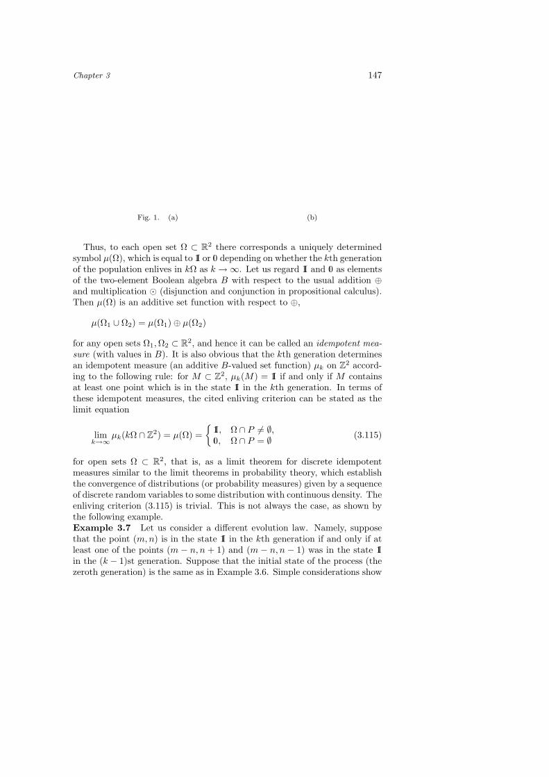
Chapter 3 147

Fig. 1. (a) (b)

Thus, to each open set Ω ⊂ R2 there corresponds a uniquely determinedsymbol µ(Ω), which is equal to 1I or 0 depending on whether the kth generationof the population enlives in kΩ as k →∞. Let us regard 1I and 0 as elementsof the two-element Boolean algebra B with respect to the usual addition ⊕and multiplication ¯ (disjunction and conjunction in propositional calculus).Then µ(Ω) is an additive set function with respect to ⊕,

µ(Ω1 ∪ Ω2) = µ(Ω1)⊕ µ(Ω2)

for any open sets Ω1, Ω2 ⊂ R2, and hence it can be called an idempotent mea-sure (with values in B). It is also obvious that the kth generation determinesan idempotent measure (an additive B-valued set function) µk on Z2 accord-ing to the following rule: for M ⊂ Z2, µk(M) = 1I if and only if M containsat least one point which is in the state 1I in the kth generation. In terms ofthese idempotent measures, the cited enliving criterion can be stated as thelimit equation

limk→∞

µk(kΩ ∩ Z2) = µ(Ω) =

1I, Ω ∩ P 6= ∅,0, Ω ∩ P = ∅ (3.115)

for open sets Ω ⊂ R2, that is, as a limit theorem for discrete idempotentmeasures similar to the limit theorems in probability theory, which establishthe convergence of distributions (or probability measures) given by a sequenceof discrete random variables to some distribution with continuous density. Theenliving criterion (3.115) is trivial. This is not always the case, as shown bythe following example.Example 3.7 Let us consider a different evolution law. Namely, supposethat the point (m,n) is in the state 1I in the kth generation if and only if atleast one of the points (m − n, n + 1) and (m − n, n − 1) was in the state 1Iin the (k − 1)st generation. Suppose that the initial state of the process (thezeroth generation) is the same as in Example 3.6. Simple considerations show

148 Chapter 3

that in the kth generation the points in the state 1I lie on the rays issuingfrom the points

(m,n) : m = k(−1)ε1 + (k − 1)(−1)ε2 + · · ·+ (−1)εk ,

n = (−1)ε1 + · · ·+ (−1)εk , εj = 0, 1with slope 1/k or parallel to the axis n = 0.

Let us try to describe the sets Ω = Ωx × Ωy ⊂ R2, where Ωx and Ωy areopen intervals, such that the set Ωk = k2Ωx×kΩy contains points in the state1I in the kth generation as k → ∞. It turns out that this is true if and onlyif Ω has a nonempty intersection with the set

Q = (|x− y| ≤ 12 ∪ |y| ≤ 1) ∩ x ≥ 1

4 (y + 1)2 − 12 ⊂ R2

(see Fig. 1 (b), where Q is dashed). The corresponding limit theorem foridempotent discrete measures µk determined (as in Example 3.6) by the kthgenerations has the form

limk→∞

µk(k2Ωx × kΩy ∩ Z2) = µ(Ω) =

1I, Ω ∩Q 6= ∅,0, Ω ∩Q = ∅ (3.116)

for any open sets Ω = Ωx × Ωy ⊂ R2.Apparently, the limit equation (3.116) can readily be obtained from the

explicit expression for the kth generation and for the measure µk, by analogywith the derivation of the de Moivre–Laplace limit theorem in probabilitytheory from the Bernoulli distribution by passing to the limit. However, thestraightforward evaluation of the limit is rather complicated in this example.We derive Eq. (3.116) from the general theory of the differential Bellmanequation by carrying out the following steps.

1) We rewrite the evolution law for the process in question as a discreteBellman equation, linear in the semimodule of functions Z2 → B.

2) We embed B as a subsemiring in the semiring A = R ∪ +∞ with theoperations a ⊕ b = min(a, b) and a ¯ b = a + b by identifying the elements0, 1I ∈ B, respectively, with the neutral elements 0 = +∞ and 1I = 0 in A.

3) We consider the auxiliary problem, namely, a process in the semimoduleof A-valued functions on R2 coinciding with the original process at the pointsof the integral lattice. The discrete Bellman equation satisfied by this processproves to be a finite-difference approximation to some differential Bellmanequation.

4) Using Pontryagin’s maximum principle and the theory developed in §3.2,we find the generalized solution of the resultant differential Bellman equationin a closed form; this solution is the limit of the discrete process in the idem-potent measure, and the set Q is the support of this solution.

Thus, consider the discrete Bellman equation

ak+1(M, N) = minv∈V

ak(M − CN,N − v)

Chapter 3 149

on the lattice M ∈ Zn, N ∈ Zn, where V ⊂ Zn is a finite set and C is an m×nmatrix of integers. Consider the following auxiliary equation for functions ofcontinuous arguments, depending on the parameter h > 0:

Sh(t + h, x, y) = min

v∈VSh(t, x− hCy, y − hv),

Sh(0, x, y) = S0(x, y).

For t = kh, we obtain

Sh(kh, x, y)

= minv1,...,vk

S0

(x− khCy − (k − 1)h2Cv1 − · · · − h2Cvk−1, y − h

k∑

i=1

vi

).

Now let

kh = t0, k →∞, h = t0/k → 0.

Then it follows from Theorem 3.3 that the sequence Sh(t0, x, y) convergesin measure of open bounded sets to a generalized solution of the differentialBellman equation

∂S

∂t+

⟨Cy,

∂S

∂x

⟩+ max

v∈V

⟨v,

∂S

∂y

⟩= 0. (3.117)

This solution has the form

S(t0, x, y) = infS0(ξ, η) : (ξ, η) ∈ K(t0, x, y),

where K(t0, x, y) is the section by the plane t = t0 of the integral funnel ofthe generalized differential equation

x = −Cy, x(0) = x0,y ∈ − co V, y(0) = y0,

in which co V is the convex hull of V , so that

limh→0

inf(x,y)∈Ω

Sn(t0, x, y) = inf(x,y)∈Ω

S(t0, x, y) (3.118)

for open bounded sets Ω ⊂ Rn+m.Suppose that the initial state of the process ak is given by a homogeneous

function a0(M, N),

a0(mM, nN) = a0(M, N) ∀m,n ∈ N.

Let S0(x, y) be a function homogeneous in x and y and coinciding with a0(x, y)at the integral points. Then

Sh(kh, kM, kN) = ak(M, N).

150 Chapter 3

It is easy to show that the infimum on the left-hand side in (3.118) can thenbe taken over the set

(x, y) ∈ Ω ∩ h2Zm × hZn,which yields the following limit equation for the process ak:

limk→∞

inf(M,N)∈Dk(Ω)

ak(M, N) = inf(x,y)∈Ω

S(1, x, y), (3.119)

where Dk(Ω) is the image of Ω under the action of the operator Dk given by

the matrix(

k2 00 k

).

In particular, the process considered in Example 3.7 obviously satisfies theequation

ak+1(m,n) = min(ak(m− n, n− 1), ak(m− n, n + 1)),

for which the limit differential equation (3.117) has the form

∂S

∂t+ y

∂S

∂x+

∣∣∣∣∂S

∂y

∣∣∣∣ = 0.

The solution of the Cauchy problem for this equation can be evaluated in aclosed form, and Eq. (3.116) follows from Eq. (3.119) (see [?] for details).