Chapter 3

Introduction to Linear Programming

Operations Research: Applications and Algorithms

4th edition

by Wayne L. Winston

Alip Mohammed, Department of Mathematics and Statistics, York University

2

3.1 What Is a Linear Programming Problem?

Linear Programming (LP) is a tool for solving optimization problems.

Linear programming problems involve important terms that are used to describe linear programming.

3

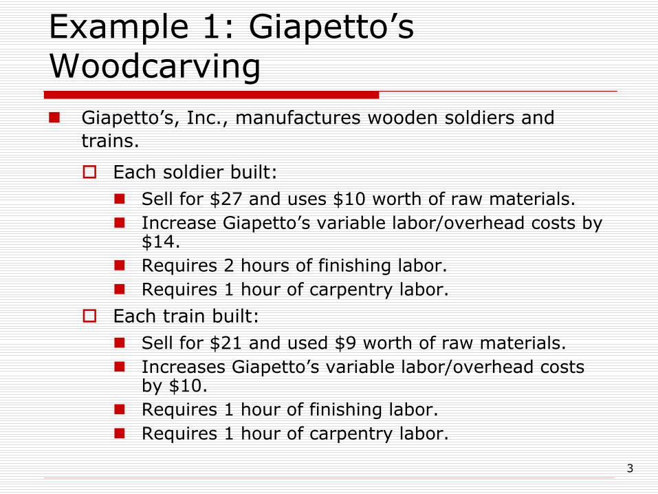
Example 1: Giapetto’s Woodcarving

Giapetto’s, Inc., manufactures wooden soldiers and trains.

Each soldier built:

Sell for $27 and uses $10 worth of raw materials.

Increase Giapetto’s

variable labor/overhead costs by $14.

Requires 2 hours of finishing labor.

Requires 1 hour of carpentry labor.

Each train built:

Sell for $21 and used $9 worth of raw materials.

Increases Giapetto’s

variable labor/overhead costs by $10.

Requires 1 hour of finishing labor.

Requires 1 hour of carpentry labor.

4

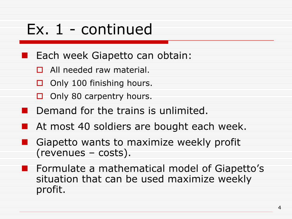
Ex. 1 -

continued

Each week Giapetto

can obtain:

All needed raw material.

Only 100 finishing hours.

Only 80 carpentry hours.

Demand for the trains is unlimited.

At most 40 soldiers are bought each week.

Giapetto

wants to maximize weekly profit

(revenues –

costs).

Formulate a mathematical model of Giapetto’s

situation that can be used maximize weekly profit.

5

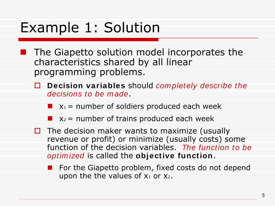
Example 1: Solution

The Giapetto solution model incorporates the characteristics shared by all linear programming problems.

Decision variables should completely describe the decisions to be made.

x1 = number of soldiers produced each week

x2 = number of trains produced each week

The decision maker wants to maximize (usually revenue or profit) or minimize (usually costs) some function of the decision variables. The function to be optimized is called the objective function.

For the Giapetto

problem, fixed costs do not depend upon the the values of x1

or x2

.

6

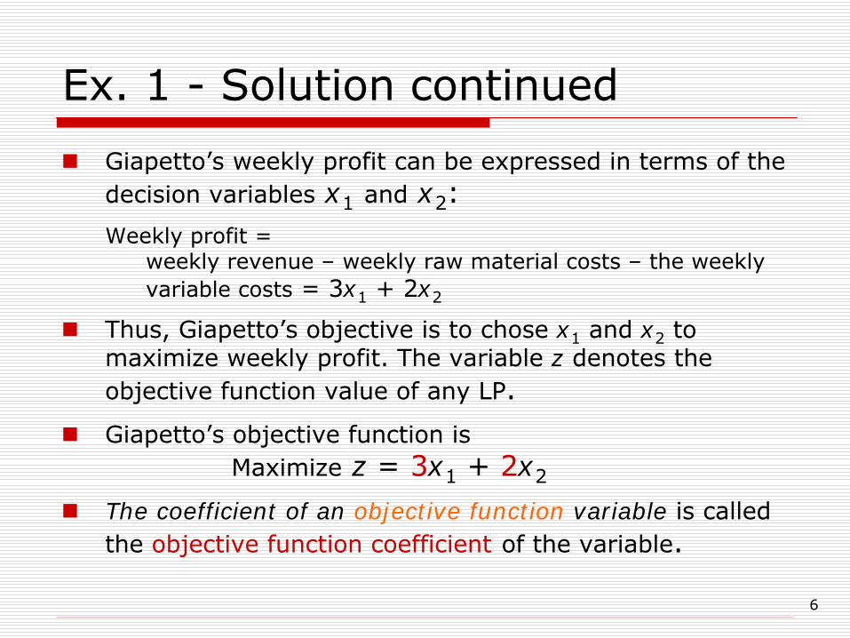
Ex. 1 -

Solution continued

Giapetto’s weekly profit can be expressed in terms of the decision variables

x1

and

x2

:Weekly profit =

weekly revenue –

weekly raw material costs –

the weekly variable costs

= 3x1

+ 2x2

Thus, Giapetto’s

objective is to chose x1

and x2

to maximize weekly profit. The variable z denotes the objective function value of any LP.

Giapetto’s

objective function is Maximize

z = 3x1

+ 2x2

The coefficient of an objective function variable is called the objective function coefficient

of the variable.

7

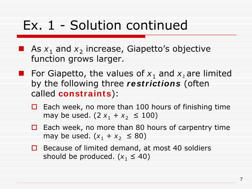
Ex. 1 -

Solution continued

As x1

and x2

increase, Giapetto’s objective function grows larger.

For Giapetto, the values of x1

and x2

are limited by the following three restrictions (often called constraints):

Each week, no more than 100 hours of finishing time may be used. (2 x1

+ x2

≤

100)

Each week, no more than 80 hours of carpentry time may be used. (x1

+ x2

≤

80)

Because of limited demand, at most 40 soldiers should be produced. (x1

≤

40)

8

The coefficients of the decision variables in the constraints

are called the technological coefficients. The number on the right-hand side of each constraint is called the constraint’s right-hand side (or rhs).

To complete the formulation of a linear programming problem, the following question must be answered for each decision variable.

Can the decision variable only assume nonnegative values, or is the decision variable allowed to assume both positive and negative values?

If the decision variable can assume only nonnegative values, the sign restriction xi

≥

0 is added.

If the variable can assume both positive and negative values, the decision variable xi

is unrestricted in sign (often abbreviated urs).

9

Ex. 1 -

Solution continued

For the Giapetto problem model, combining the sign restrictions x1

≥0 and x2

≥0 with the objective function and constraints yields the following optimization model:

Max z = 3x1

+ 2x2

(objective function)

Subject to (s.t.)2 x1

+ x2

≤

100

(finishing constraint)

x1

+ x2

≤

80

(carpentry constraint)

x1

≤

40

(constraint on demand for soldiers)

x1

≥

0

(sign restriction)

x2

≥

0

(sign restriction)

10

A function f(x1

, x2

, …, xn

) of x1

, x2

, …, xn

is a linear function if and only if f(x1

, x2

, …, xn

) = c1

x1 + c2

x2

+ …

+ cn

xn

, for some set of constants, c1

, c2

, …, cn

.

For any linear function f(x1

, x2

, …, xn

) and any number b, the inequalities f(x1

, x2

, …, xn

) ≤

b and f(x1

, x2

, …, xn

) ≥

b are linear inequalities.

11

A linear programming problem (LP) is an optimization problem for which we do the following:

Attempt to maximize (or minimize) a linear function (called the objective function) of the decision variables.

The values of the decision variables must satisfy a set of constraints. Each constraint must be a linear equation or inequality.

A sign restriction is associated with each variable. For any variable xi

, the sign restriction specifies either that xi

must be nonnegative (xi

≥

0) or that xi

may be unrestricted in sign.

12

The fact that the objective function for an LP must be a linear function of the decision variables

has two implications:

1.

The contribution of the objective function from each decision variable is proportional to the value of the decision variable. For example, the contribution to the objective function for 4 soldiers is exactly fours times the contribution of 1 soldier.

2.

The contribution to the objective function for any variable is independent of the other decision variables. For example, no matter what the value of x2

, manufacturing of x1

soldiers will always contribute 3x1

dollars to the objective function.

The Proportionality & Additivity Assumptions

13

Analogously, the fact that each LP constraint must be a linear inequality or linear equation

has two implications:

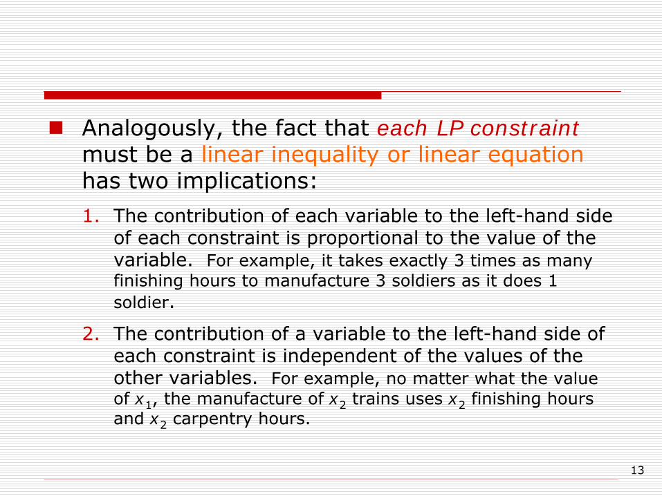
1.

The contribution of each variable to the left-hand side of each constraint is proportional to the value of the variable. For example, it takes exactly 3 times as many finishing hours to manufacture 3 soldiers as it does 1 soldier.

2.

The contribution of a variable to the left-hand side of each constraint is independent of the values of the other variables. For example, no matter what the value of x1

, the manufacture of x2

trains uses x2

finishing hours and x2

carpentry hours.

14

The first item in each list is called the Proportionality Assumption of Linear Programming.

The second item in each list is called the Additivity Assumption of Linear Programming.

The divisibility assumption requires that each decision variable be permitted to assume fractional values.

15

The certainty assumption is that each parameter (objective function coefficients, right-hand side, and technological coefficients) are known with certainty.

The feasible region of an LP is the set of all points satisfying all the LP’s constraints and sign restrictions.

For a maximization problem, an optimal solution to an LP is a point in the feasible region with the largest objective function value.

Similarly, for a minimization problem, an optimal solution is a point in the feasible region with the smallest objective function value.

16

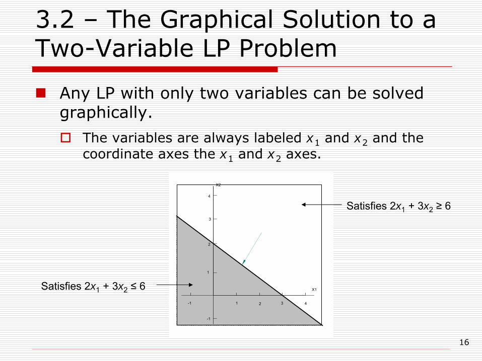
3.2 –

The Graphical Solution to a Two-Variable LP Problem

Any LP with only two variables can be solved graphically.

The variables are always labeled x1

and x2

and the coordinate axes the x1

and x2

axes.

Satisfies 2x1

+ 3x2

≥

6

Satisfies 2x1

+ 3x2

≤

6 X1

1 2 3 4

1

2

3

4

X2

-1

-1

17

Since the Giapetto

LP has two variables, it may

be solved graphically.

The feasible region is the set of all points satisfying the constraints

2 x1

+ x2

≤

100 (finishing constraint)

x1

+ x2

≤

80 (carpentry constraint)

x1

≤

40 (demand constraint)

x1

≥

0 (sign restriction)

x2 ≥

0 (sign restriction)

18

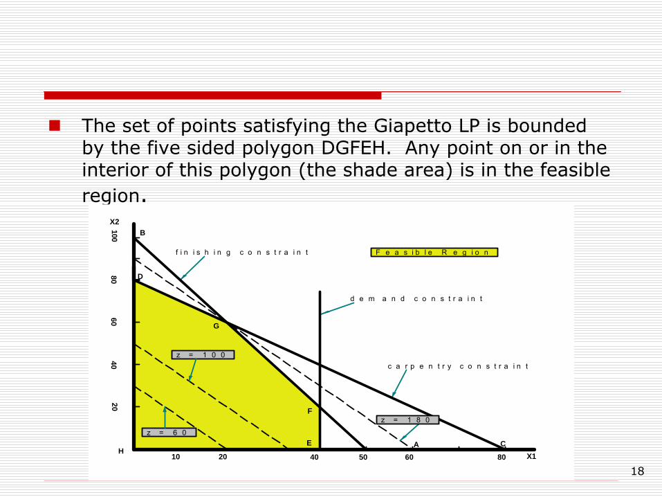
The set of points satisfying the Giapetto

LP is bounded by the five sided polygon DGFEH. Any point on or in the interior of this polygon (the shade area) is in the feasible region.

X1

X2

10 20 40 50 60 80

2040

6080

100

f i n i s h i n g c o n s t r a i n t

c a r p e n t r y c o n s t r a i n t

d e m a n d c o n s t r a i n t

z = 6 0

z = 1 0 0

z = 1 8 0

F e a s i b l e R e g i o n

G

A

B

C

D

E

F

H

19

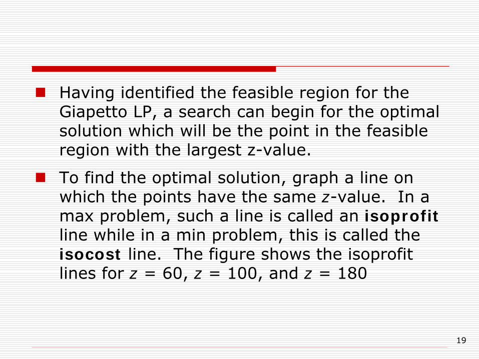
Having identified the feasible region for the Giapetto

LP, a search can begin for the optimal

solution which will be the point in the feasible region with the largest z-value.

To find the optimal solution, graph a line on which the points have the same z-value. In a max problem, such a line is called an isoprofit line while in a min problem, this is called the isocost line. The figure shows the isoprofit

lines for z = 60, z = 100, and z = 180

20

A constraint is binding if the left-hand and right-hand side of the constraint are equal when the optimal values of the decision variables are substituted into the constraint.

In the Giapetto

LP, the finishing and carpentry constraints are binding.

A constraint is nonbinding if the left-hand side and the right-hand side of the constraint are unequal when the optimal values of the decision variables are substituted into the constraint.

In the Giapetto

LP, the demand constraint for wooden soldiers is nonbinding since at the optimal solution (x1

= 20), x1 < 40.

21

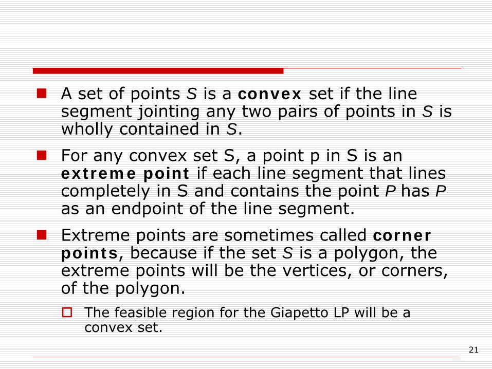
A set of points S is a convex set if the line segment jointing any two pairs of points in S is wholly contained in S.

For any convex set S, a point p in S is an extreme point if each line segment that lines completely in S and contains the point P has P as an endpoint of the line segment.

Extreme points are sometimes called corner points, because if the set S is a polygon, the extreme points will be the vertices, or corners, of the polygon.

The feasible region for the Giapetto

LP will be a convex set.

22

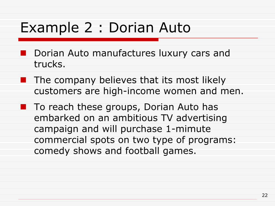
Example 2 : Dorian Auto

Dorian Auto manufactures luxury cars and trucks.

The company believes that its most likely customers are high-income women and men.

To reach these groups, Dorian Auto has embarked on an ambitious TV advertising campaign and will purchase 1-mimute commercial spots on two type of programs: comedy shows and football games.

23

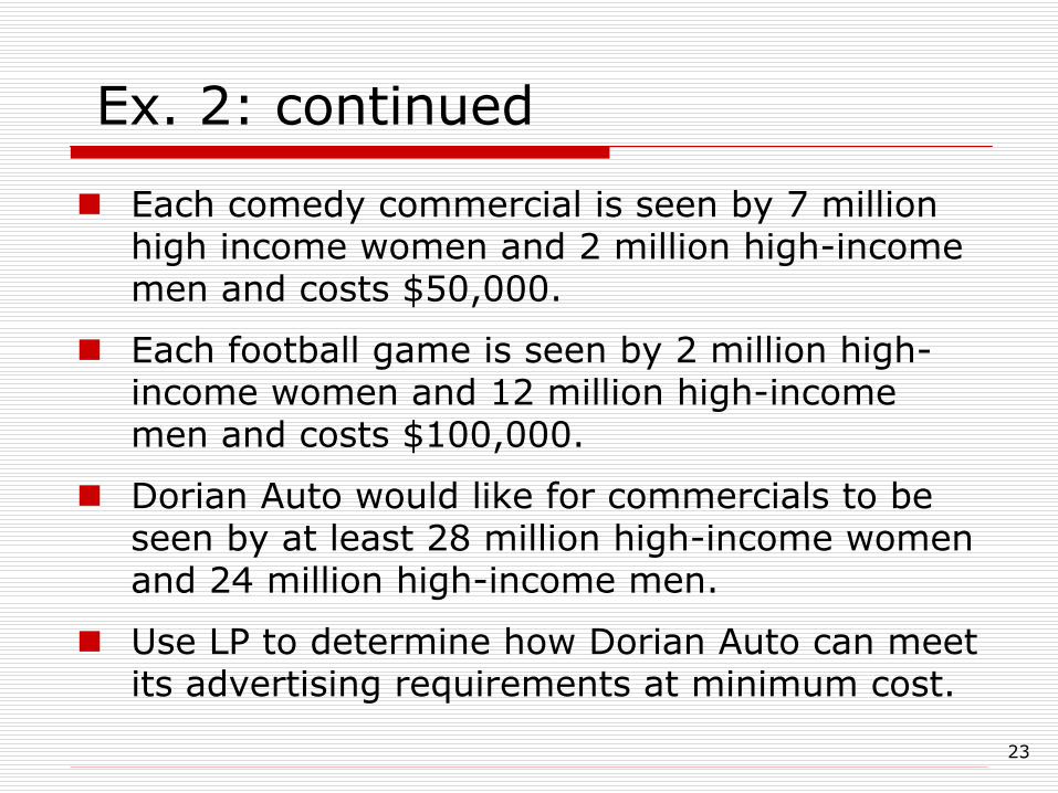
Ex. 2: continued

Each comedy commercial is seen by 7 million high income women and 2 million high-income men and costs $50,000.

Each football game is seen by 2 million high-

income women and 12 million high-income men and costs $100,000.

Dorian Auto would like for commercials to be seen by at least 28 million high-income women and 24 million high-income men.

Use LP to determine how Dorian Auto can meet its advertising requirements at minimum cost.

24

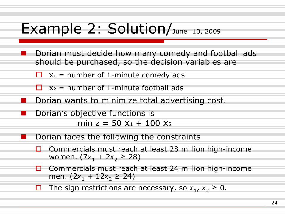
Example 2: Solution/June

10, 2009

Dorian must decide how many comedy and football ads should be purchased, so the decision variables are

x1

= number of 1-minute comedy ads

x2

= number of 1-minute football ads

Dorian wants to minimize total advertising cost.

Dorian’s objective functions is min z = 50 x1

+ 100 x2

Dorian faces the following the constraints

Commercials must reach at least 28 million high-income women. (7x1

+ 2x2

≥

28)

Commercials must reach at least 24 million high-income men. (2x1

+ 12x2

≥

24)

The sign restrictions are necessary, so x1

, x2

≥

0.

25

Ex. 2 –

Solution continued

Like the Giapetto

LP, The Dorian LP has a

convex feasible region.

The feasible region for the Dorian problem, however, contains points for which the value of at least one variable can assume arbitrarily large values.

Such a feasible region is called an unbounded feasible region.

26

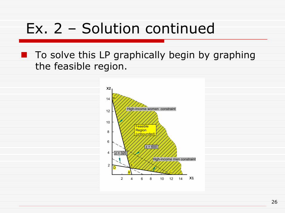
Ex. 2 –

Solution continued

To solve this LP graphically begin by graphing the feasible region.

X1

X2

2

4

6

8

10

12

14

2 4 6 8 10 12 14

z = 600

z = 320

A CD

E

B

Feasible Region (unbounded)

High-income women constraint

High-income men constraint

27

Ex. 2 –

Solution continued

Since Dorian wants to minimize total advertising costs, the optimal solution to the problem is the point in the feasible region with the smallest z value.

An isocost

line with the smallest z value passes

through point E and is the optimal solution at x1 = 3.4 and x2 = 1.4.

Both the high-income women and high-income men constraints are satisfied, both constraints are binding.

28

Does the Dorian model meet the four assumptions of linear programming?

The Proportionality Assumption is violated because at a certain point advertising yields diminishing returns.

Even though the Additivity

Assumption was used in writing: (Total viewers) = (Comedy viewer ads) + (Football ad viewers) many of the same people might view both ads, double-counting of such people would occur thereby violating the assumption.

The Divisibility Assumption is violated if only 1-

minute commercials are available. Dorian is unable to purchase 3.6 comedy and 1.4 football commercials.

The Certainty assumption is also violated because there is no way to know with certainty how many viewers are added by each type of commercial.

29

3.3 Special Cases

The Giapetto and Dorian LPs each had a unique optimal solution.

Some types of LPs do not have unique solutions.

Some LPs have an infinite number of solutions (alternative or multiple optimal solutions).

Some LPs have no feasible solutions (infeasible LPs).

Some LPs are unbounded: There are points in the feasible region with arbitrarily large (in a maximization problem) z-values.

The technique of goal programming is often used to choose among alternative optimal solutions.

30

It is possible for an LP’s feasible region to be empty, resulting in an infeasible LP.

Because the optimal solution to an LP is the best point in the feasible region, an infeasible LP has no optimal solution.

For a max problem, an unbounded LP occurs if it is possible to find points in the feasible region with arbitrarily large z-values, which corresponds to a decision maker earning arbitrarily large revenues or profits.

31

For a minimization problem, an LP is unbounded if there are points in the feasible region with arbitrarily small z-

values.

Every LP with two variables must fall into one of the following four cases.

The LP has a unique optimal solution.

The LP has alternative or multiple optimal solutions: Two or more extreme points are optimal, and the LP will have an infinite number of optimal solutions.

The LP is infeasible: The feasible region contains no points.

The LP unbounded: There are points in the feasible region with arbitrarily large z-values (max problem) or arbitrarily small z-values (min problem).

32

3.4 A Diet Problem Example 6: Diet Problem

My diet requires that all the food I get come from one of the four “basic food groups”.

At present, the following four foods are available for consumption: brownies, chocolate ice cream, cola and pineapple cheesecake.

Each brownie costs 50¢, each scoop of ice cream costs 20 ¢, each bottle of cola costs 30 ¢,, and each piece of pineapple cheesecake costs 80 ¢.

Each day, I must ingest at least 500 calories, 6 oz of chocolate, 10 oz of sugar, and 8 oz of fat.

33

Ex. 6 -

continued

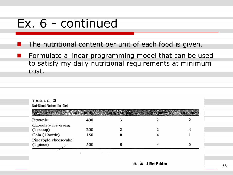
The nutritional content per unit of each food is given.

Formulate a linear programming model that can be used to satisfy my daily nutritional requirements at minimum cost.

34

Example 6: Solution

As always, begin by determining the decisions that must be made by the decision maker: how much of each type of food should be eaten daily.

Thus we define the decision variables:

x1

= number of brownies eaten daily

x2

= number of scoops of chocolate ice cream eaten daily

x3

= bottles of cola drunk daily

x4

= pieces of pineapple cheesecake eaten daily

35

Ex. 6 –

Solution continued

My objective is to minimize the cost of my diet.

The total cost of any diet may be determined from the following relation:

(total cost of diet) = (cost of brownies) + (cost of ice cream) +(cost of cola) + (cost of cheesecake).

The decision variables must satisfy the following four constraints:

Daily calorie intake must be at least 500 calories.

Daily chocolate intake must be at least 6

oz.

Daily sugar intake must be at least 10 oz.

Daily fat intake must be at least 8 oz.