Ch 3. Dynamic Features and Methods of Analysis

3−1

Chapter 3 Dynamic Features and Methods of Analysis

3.1 Introduction

3.1.1 Fluid transport phenomena

= ability of fluids in motion to

= mechanism by which materials and properties are

convey materials and properties from place to place

diffused and transmitted through the

fluid medium

because of molecular motion

process

mass transport

observational law

conservation of matter

heat transport conservation of energy (1st law of thermodynamics)

momentum transport equation of motion (Newton's 2nd law)

Transport of materials and properties in the direction of decreasing mass, temperature, momentum

{ } ( )/ /dM dt d M volqarea ds

= ∝

Flux = quantity per unit time per area

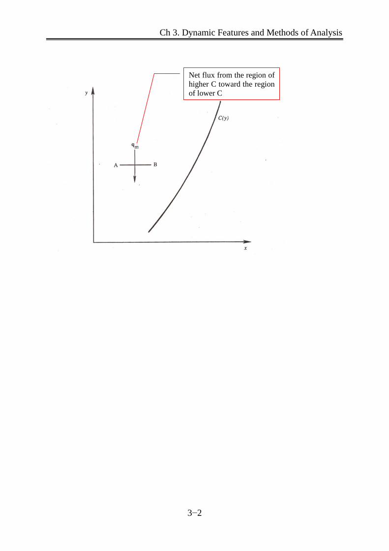
Ch 3. Dynamic Features and Methods of Analysis

3−2

Net flux from the region of higher C toward the region of lower C

Ch 3. Dynamic Features and Methods of Analysis

3−3

Molecular motion at the surface

Turbulent motion at the surface

Net flux: m

cqy∂

∝∂

Random, irregular migration of molecules

Fluid parcel

Ch 3. Dynamic Features and Methods of Analysis

3−4

3.1.2 Subsidiary Laws

→ Relations between fluxes and driving force (gradient)

→ Transport analogy

Flux Driving force Law Relation

Mass flux mq

concentration gradient

j

cx∂∂

Fick's law m

j

cq D D cx∂

= − = − ∇∂

Heat flux Hq

temperature gradient

j

Tx∂∂

Fourier's law H

j

Tq k k Tx∂

= − = − ∇∂

Momentum Flux, moq

velocity gradient

i

j

ux∂∂

Newton's law i

j

ux

τ µ ∂=

∂

◈ momentum flux

( )( / )

momu m u t ma Fq stress

t x y A A Aτ= = = = = =

∆ ∆ (3.1)

Mass/heat transport:

c, T – scalar

,m Hq q - vector

momentum transport:

iu – vector

moq τ= - tensor

Ch 3. Dynamic Features and Methods of Analysis

3−5

3.2 Mass Transport

All fluid motions must satisfy the principle of conservation of matter.

homogeneous fluid single phase

non-homogeneous fluid multi phase: air-liquid, liquid-solid

multi species: fresh water - salt water

Homogeneous fluid Non-homogenous fluid

single phase multi phase

single species single phase & multi species

[Ch. 4] Continuity Equation

mass transport due to local velocity

+ mass transport due to diffusion

→ [Advanced Environmental Hydraulics]

Advection-Diffusion Equation

Continuity equation: relation for temporal and spatial variation of velocity and density

( ) 0qtρ ρ∂+∇⋅ =

∂

Advection-Diffusion Equation

= Advection + molecular diffusion

0c cuc Dt x x

∂ ∂ ∂ + =− ∂ ∂ ∂

'u u u= +

Mean motion fluctuation

' 'd

cq u c Dx∂

= =∂

Ch 3. Dynamic Features and Methods of Analysis

3−6

3.3 Heat Transport

thermodynamics ~ non-flow processes

equilibrium states of matter

fluid dynamics ~ transport of heat (scalar) by fluid motion

• Apply conservation of energy to flow process (= 1st law of thermodynamics)

~ relation between pressure, density, temperature, velocity, elevation, mechanical work, and

heat input (or output).

~ since heat capacity of fluid is large compared to its kinetic energy, temperature and density

remain constant even though large amounts of kinetic energy are dissipated by friction.

→ simplified energy equation

• Heat transfer in flow process

1) convection: due to velocity of the flow – advection

2) conduction: analogous to diffusion, tendency for heat to move in the direction of

decreasing temperature

• Application

1) Fluid machine (compressors, pumps, turbines): energy transfer in flow processes

2) Heat pollution: discharge of cooling water for nuclear power plant

[Re] Thermal stratification

- Ocean, lake, reservoir

- density variations

Ch 3. Dynamic Features and Methods of Analysis

3−7

Nuclear Power Plant

Ch 3. Dynamic Features and Methods of Analysis

3−8

3.4 Momentum Transport

3.4.1 Momentum transport phenomena

~ encompass the mechanisms of fluid resistance, boundary and internal shear stresses

, and

propulsion and forces on immersed bodies.

Momentum mass velocity vector mu= ⋅ =

Adopt Newton's 2nd law

( )du dF ma m mudt dt

= = =∑

(3.2)

→ Equation of motion

• Effect of velocity gradient uy∂∂

- macroscopic fluid velocity tends to become uniform due to the random motion of molecules

because of intermolecular collisions and the consequent

→ the velocity distribution tends toward the dashed line

exchange of molecular momentum

→ momentum flux is equivalent to the existence of the shear stress

uy

τ ∂∝∂

uy

τ µ ∂=∂

→ Newton’s law of friction

Ch 3. Dynamic Features and Methods of Analysis

3−9

Ch 3. Dynamic Features and Methods of Analysis

3−10

3.4.2 Momentum transport for Couette flow

Couette flow – laminar flow between two plates

transverse transport of longitudinal momentum ( )mv

∝ transverse gradient of longitudinal velocity dvdy

in the direction of decreasing velocity (longitudinal momentum)

[Re] velocity gradient of Couette flow

- linear

dv Udy a

=

No slip: 0v =

No slip: v U=

U

a

F∆

Ch 3. Dynamic Features and Methods of Analysis

3−11

3.5 Transport Analogies

(1) Transport

1) advection = transport by imposed current (velocity)

[cf ] convection

2) diffusion = movement of mass or heat or momentum in the direction of decreasing

concentration of mass, temperature, or momentum

[cf] conduction

(2) Driving force (= gradient)

{ } ( )/ /dM dt d M volfluxarea ds

= ∝

( )// d M voldM dt KA ds

= (3.3)

where K = diffusivity constant ( )2 2/ /m S L t

K = f (modes of fluid motion, i.e., laminar and turbulent flow)

molecular diffusivity for laminar flow

turbulent diffusivity for turbulent flow

mass, heat, momentum

Gradient of M per unit volume of fluid in the transport direction

Flux = Time rate of transport of M per unit area normal to transport direction

Ch 3. Dynamic Features and Methods of Analysis

3−12

3.5.1 Momentum transport

Set momentumM mu= = ∆

( ) 1d mu d muKdt x z dy vol∆ ∆ ∴ = ∆ ∆ ∆

Now, apply Newton's 2nd law to LHS

( )d dumu m ma Fdt dt

= = =

( )x

d muF

dt∆

∴ = ∆

( )x

yx

d muFdtLHS

x z x zτ

∆∆

∴ = = =∆ ∆ ∆ ∆

yxτ = shear stress parallel to the x-direction acting on a plane

whose normal is parallel to y-direction

RHS:

mvol

ρ∆=

∆

( )d ud muRHS K K

dy vol dyρ∆ ∴ = = ∆

Combine (i) and (ii)

( )

yxd u

Kdyρ

τ = (3.4)

Ch 3. Dynamic Features and Methods of Analysis

3−13

If ρ = constant

yxduKdy

τ ρ= (3.5)

K = molecular diffusivity constant 2m / s( )

If kinematic viscosityK v µρ

≡ = =

Then,

yxdu duvdy dy

τ ρ µ= = (3.6)

3.5.2 Heat transport

upper plate ~ high temperature

lower plate ~ low temperature

Set

heat pM Q mC T= = = ∆ (3.7)

where pC = specific heat at constant pressure

Then, Eq. (3.3) becomes

1

y

pH

mC TdQ dq Kdt x z dy vol

∆ = = − ∆ ∆ ∆

(3.8)

Hq = time rate of heat transfer per unit area normal

to the direction of transport ( )2/ sec mj −

conduction of heat within fluid

Ch 3. Dynamic Features and Methods of Analysis

3−14

thermal diffusivityK α= = ( )2m / sec

If ( )mvol

ρ ∆=∆

and pC = const.

Hy pdT dTq C K kdy dy

ρ∴ = − = − (3.9)

where pk C Kρ= = thermal conductivity ( )/ sec mj K− −

3.5.3 Mass transport

Set

dissolved mass of substancs f MM m C= = ∆ (3.10)

where fm∆ = mass of fluid

MC = concentration

≡ mass of dissolved substance /unit mass of fluid

[Cf] (mg / , )ss

f

mC l ppmvol∆

=∆

Then, Eq. (3.3) becomes

( ) 1

y

f M f MM

d m C m Cdj Kdt x z dy vol

∆ ∆ = = − ∆ ∆ ∆

(3.11)

Ch 3. Dynamic Features and Methods of Analysis

3−15

Mj = time rate or mass transfer per unit area normal to the direction

of transport 2kg/m s⋅

If const. = f

f

mmvol vol

ρ∆∆

= =∆ ∆

y

MM

dCj Kdy

ρ= − (3.12)

fs s

f f f sM

mm md dm vol vol dCdCK K K K

dy dy dy dyρ

∆ ∆ ∆ ⋅ ∆ ∆ ∆⋅ = − = − = − = −

Set K D= = molecular diffusion coefficient ( )2m / sec

y

M sM

dC dCj K Ddy dy

ρ= − = −

transport process kinematic fluid property 2( / s)m

momentum ν (kinematic viscosity)

heat α (thermal diffusivity)

mass D (diffusion coefficient)

Ch 3. Dynamic Features and Methods of Analysis

3−16

3.6 Particle and Control-Volume Concepts

3.6.1 Infinitesimal elements and control volumes

- Eulerian equations

(1) Material method: particle approach

of fluid mechanics

~ describe flow characteristics at a fixed point ( , , )x y z by observing the motion

of a

~ laws of conservation of mass, momentum, and energy can be stated in the differential form,

applicable at a

material particle of a infinitesimal mass

point

~ Newton's 2nd law

.

dF dma=

◦ If fluid is considered as a continuum, end result of either method is identical

.

(2) Control volume method

① differential (infinitesimal) control volume – parallelepiped control volume

② finite control volume – arbitrary control volume

[Re] Control volume

- fixed volume which consists of the same fluid particles and whose bounding surface

moves with the fluid

Ch 3. Dynamic Features and Methods of Analysis

3−17

① Differential control volume method

~ concerned with a fixed differential control volume ( )x y z= ∆ ∆ ∆ of fluid

~ 2–D or 3–D analysis, Ch. 6

( ) ( )d dF mq x y zqdt dt

ρ∆ = ∆ = ∆ ∆ ∆

~ , ,x y z∆ ∆ ∆ become vanishingly small

→ point form

of equations for conservation of mass, momentum, and energy

② Finite control volume method

→ frequently used for 1–D analysis, Ch. 4

~ gross descriptions of flow

~ analytical formulation is easier than differential control volume method

~ integral form of equations for conservation of mass, momentum, and energy

Ch 3. Dynamic Features and Methods of Analysis

3−18