CHAPTER 3

Computer Simulation of Management Systems

If you have patiently proceeded from, one chapter to the next, you

have studied a perhaps bewildering variety of operations research models

and techniques. Students often ask, in effect, “Is this arsenal of tools powerful

enough to encompass all the important managerial decision problems requiring

data analysis?” The answer is no, not by a long shot. To see why, reflect on

the kinds of problems that you know can be effectively analyzed by the

operations research tools presented thus far. As you become aware of gaps,

you will see more clearly why so many significant types of decision-analysis

problems are still not solvable by these approaches, and therefore must be

attacked in other ways. In the next few para-graphs we summarize the limitations

as well as the strengths of operations research tools including linear and

dynamic programming, inventory and queuing theory.

You have already learned that linear programming models are most

successful in aiding the planning efforts of corporate enterprises. If the planning

horizon is 10 years or longer, a corresponding multiperiod linear programming

model typically deals only with annualized data. The effects of the resultant

plan on week-to-week and month-to-month operations are left implicit.

Analogously, if the planning horizon is much shorter, say three months to a

year, the corresponding model usually ignores the day-to-day and week-to

week variations. Thus, for the most part, linear programming analysis falls

short of prescribing rules that translate a recommended plan into operating

57

procedures for time spans shorter than the periods in the model.

A second limitation of linear programming analysis relates to uncertainty

about the future. Imprecise forecasts to some degree exist in all planning

studies.

Frequently, this uncertainty is not really the essence of the planning

problem, or it reflects a lack of knowledge about only a few parameters in the

model. In such cases, sensitivity analysis, as discussed in Chap. 5, suffices

to determine the impact of uncertainty. But on other occasions uncertainty

pervades the entire model, and standard sensitivity analysis is too clumsy

and computationally burdensome for analyzing the impact of uncertainty.

To rllustrate. consider a chemical manufacturing company that seeks a

long-range strategy for the development and marketing of new products.

Substantial research and investment costs are associated with each product,

and the actual size of the product’s market is uncertain. Furthermore, most

of the profits that are generated from a successful product will be used to

finance the research and development of new products. A linear programming

model that manages to capture the dynamic elements of this situation, but

treats the uncertainty aspects by simply using average values, is not likely to

yield a good strategy.

In contrast, dynamic programming models can analyze multiperiod

planning problems containing uncertainty, and so can be used to determine

optimal strategies. But, as compared with linear programming applications,

these dynamic programming models in practice can treat only drastically

58

simplified systems. As you learned in Chaps. 10 and 1 7, unless the underlying

system is characterized by only a few state variables, the computational task

of solving a dynamic pro-gramming model is horrendous.

A similar limitation holds for those dynamic probabilistic models that

are amenable to mathematical analysis, such as the inventory and queuing

phenomena you studied in Ghaps. 19 and 20. To solve these models, you

not only must restrict yourself to a small-scale system, but you also must

simplify the way the system can operate. To illustrate, a realistic analysis of

waiting lines in a job-shop is intract-able using mathematical queuing theory

like that presented in Chap. 20 and Appendix III. Those models serve only

as rough approximations to realistic queuing phenomena.

Thus, despite the great diversity of applications of mathematical

programming and probabilistic models, many important managerial decision-

making problems must be analyzed by other kinds of techniques.

3.1 CHALLENGE REMAINING. The expanding scientific literature on

operations research bears witness that there is steady progress in finding

techniques to overcome the above-mentioned limitations. But for now and

the foreseeable future, the approaches given in the preceding chapters cannot

be relied on to provide a complete analysis of managerial decision-making

problems pertaining to:

(i) Choice of Investment Policies for Strategic Planning. A major

corporation’s invest-ment policy, to be comprehensive, should include

59

provisions relating to research and development of new products, expansion

into new markets, choice of selec-tion criteria for major projects, measurement

and evaluation of risk, means of financing by debt and equity, reinvestment

of earnings, disposition of liquid assets, evaluation of mergers and acquisitions,

and divestment of assets. A full-fledged operations research model for the

analysis of alternative policies must recognize the impact of the uncertain and

dynamic nature of investments, as well as provide a means for screening the

enormous variety of investment decisions that face an organization.

(ii) Selection of Facilities in Operations Planning. Several examples in

this category were already discussed in Sec. 20.1. They included the

determination of the num-ber of checkout stands in a supermarket, the number

of gasoline pumps at a service station, and the number of elevators in a new

office building. There are numerous other examples dealing with personnel

staffing, plant layout, and machine capacity decisions. Typical facilities

selection questions are of the form: “How many?” “How large?” “Where

located?”

(iii) Design of Information-Feedback Scheduling and Operations Rules.

Illustrations of decision problems in this category are equally numerous,

although you may not think of them right away, unless you have had some

previous work experience. An important example is the design of scheduling

rules for a job-shop manufactur-ing plant, or an equipment repair facility, or a

computer center. Such rules for a manufacturing plant take account of

promised due dates to customers, the requirements for, and the availabilities

60

of, machine capacities, the deployment of skilled labor, and the provisioning

for raw materials. As information on new orders arrives, and as completed

orders leave the system, the shop schedule has to be updated and revised.

Another example of an information-feed back system is a scheduling

procedure for routing transport facilities. To illustrate a freighter shipping

company in making a schedule of its ocean going equipment for several

months ahead, must take into account cargo demands at various ports, ship

capacities and speeds, uncertainties in sailing times due to vagaries in the

weather, and delays due to port congestion. Many shipping lines that own a

large fleet of vessels must reschedule daily as they receive more accurate

information about uncertain events. Similar problems arise in the scheduling

of patients into a hospital, and the timing of traffic lights on a majpr

thoroughfare.

What makes the three types of problems described above so difficult

to analyze? It is the combined effect of uncertainty, the dynamic interactions

between deci-sions and subsequent events, the complex interdependencies

among the variables in the system, and, in some instances, the need to use

finely divided time intervals. Such total systems problems are too big and

too intricate to handle with linear and dynamic programming models, or

standard probabilistic models.

Frequently, actual decisions arising from these three types of problems

involve spending at least several hundred thousand dollars, and vitally affect

the future operating costs and efficiencies of a company. Thus, management

61

is highly moti-vated to employ a systematic approach to improve on intuitive,

or “seat-of-the-pants,” analysis. So far, the best operations research

approach available is digital computer simulation, Simulation approach.

Our main concern in this chapter will be to describe simulation and the kinds

of problems you encounter in employing this technique. We do not show

you in detail how to design and run simulations. Such instructions are in texts

devoted to simulation and in manuals distributed by computer manufacturers

to explain special simulation programming languages.

In brief, the simulation approach starts by building an experimental

model of a system. Then various specific alternatives are evaluated with

reference to how well they fare in test runs of the model.

If you think about it, you will recall occasions when you have been

involved in a simulated environment. For example, an amusement park, like

Disneyland, offers you many attractions, such as the jungle boat-ride and the

Matterhorn bobsled, that try to simulate actual experience. Less frivolous

examples are planetarium shows and the environments in a museum of natural

history. You may have learned how to drive an automobile in a mock-up

mechanism with a steering wheel and gas and brake pedals. And if you have

been in the armed services, you will remember that boot camp or basic

training consists mainly of simulated exercises.

It is usually too inconvenient and expensive to solve managerial decision

prob-lems by environmental analogue simulations, such as the field combat

war games that arc used in boot camp and basic training. Rather, it is preferable

62

to represent a complex system by a computerized mathematical model. In a

computer, the only thing that can be shot is an electronic circuit.

The uncertainties, dynamic interactions, and complex interdependences

are all characterized by formulas stored in the memory of the high-speed

digital electronic computer. The system simulation begins at a specified starting

state. The combined effects of decisions, and of controllable and

uncontrollable evems, some of which may be random, cause the system to

move to another state at a future instant in time. The evolutionary process

continues in this fashion until the end of the horizon. Frequently, the time

intervals are finely divided and extend over a fairly long horizon. As a

consequence, the simulation experiments involve a vast number of calculations,

rapidly performed by the computer. This feature of years of history evolving

in a few minutes on a computer is termed time com-pression.

The only game in town. Most operations research analysts look

upon digital computer simulation as a “method of last resort”—hence the

title of this section, “When All Else Fails. . . .” There are two reasons for this

gloomy attitude.

The first reason is the nature of most simulation results. When the

model includes uncertain events, the answers stemming from a particular

simulation must be viewed only as estimates subject to statistical error. For

example, a simu-lated queuing model yields only an estimate of a waiting

line’s average length or the associated probability of a delay. Therefore, when

63

you draw conclusions about the relative merit of different specific trial policies

as tested by a simulation model, you must be careful to assess the

accompanying random variations.

The second reason for diffidence about simulation involves the nature

of the applications themselves. If a system is so complicated that it is beyond

the reach, of such operations research tools as linear and dynamic programming

or standard probability analysis, then the required model-building effort and

the subsequent analysis of the simulated results are likely to be difficult.

Many an unwary analyst has found, to his chagrin, that the simulated world is

as unfathomable as the real world he hoped to approximate—he allowed so

much to go on in the model that it hampered his finding any insightful

information.

The above two reasons also suggest why electronic computers are

indispensable in performing simulations. To obtain sufficient statistical

accuracy for reliable decisions, a considerable number of simulation runs are

usually necessary. Each experiment is so complicated that it would be virtually

impossible to perform the simulation manually in a reasonable period of time.

It is not surprising, then, that computer simulation is often an expensive way

to study a complex system.

3.2 SIMULATION IN PERSPECTIVE

As you read in the preceding section, many important managerial

decision problems are too complex and too large to be solved by

mathematical program-ming and standard probability analysis. In such cases,

64

real-life experimentation, even if feasible, is usually too costly a way to analyze

the alternatives. These observations establish the need for other problem-

solving approaches, but do not by themselves justify computer simulation.

Here we discuss why computer simulation is a useful technique, as well as

what its limitations are.

Unlike the situation with mathematical programming, there are as yet

no underlying principles guiding the formulation of simulation models. Each

ap-plication is ad hoc to a large extent. Computer simulation languages come

the closest to providing any general guidelines. [SIMSCRIPT and the General

Purpose Systems Simulator (GPSS) are the two best-known languages; we

say more about these programs in Sec. 21.8.]

The absence of a unifying theory of digital simulation is both a boon

and a bane. On the positive side, you can build a simulation model containing

arbi-trarily high-order complexities and a huge number of dynamic inter

dependencies, as well as nonstationarities and correlated random phenomena.

On the negative side, the more complicated the model, the more you will

have to rely on em-bryonically developed statistical theory to perform the

data analyses. As mentioned above, the very intricacy of the model can make

it difficult to assess the model’s validity. If the model is very complicated,

you may have to expend a great deal of computer time on replication to

obtain trustworthy answers and nearly optimal policies. Given the considerable

research interest in simulation techniques, how-ever, many of the current

deficiencies in the theory and design of simulation experiments are bound to

65

be eliminated in the years ahead.

Objectives. You would construct a simulation model to assist in

analyzing managerial decision problems with one or more of the following

purposes in mind:

(i) To Describe a Current System. Consider a manufacturing firm that

recently has witnessed an increase in its customer orders, and has noticed a

consequent marked deterioration in meeting due-dates promised to its

customers. This company may want to build a simulation model to study

how its current procedures for estimating due-dates, scheduling production,

and ordering raw material are giving rise to the observed delays.

(ii) To Explore a Hypothetical System. Consider a hospital that is

contemplating the installation of a new computerized inventory replenishment

system for its medical supplies. It may want to build a simulation model

using historical data to test what the average level of inventory investment

would be, and how often there would be shortages of various supplies under

the proposed plan.

(iii) To Design an Improved System. Consider a job shop in which

machine capacities are allocated by priorities assigned to each job. The

company may want to build a simulation model in order to find an effective

way to assign such priorities so that the jobs are completed without long

delays and, at the same time, so that equipment utilization is acceptably high.

We turn next to the steps in constructing and applying a simulation model.

So you want to build a simulation. The outline to follow describes the way

66

you would go about constructing a simulation:

Step 1. Formulate the Model. This step is much the same as that for

other opera-tions research models. There is an ever-present danger, however,

of including too much detail in a simulation model and, as a result, consuming

excessive amounts of computer time to perform the experiments. The best

guard against this tendency is to keep your specific purpose constantly in

mind. For example, if a model is to aid in the choice between two different

locations for a new warehouse, it is probably not necessary to simulate

activities on a hour-to-hour, or even day-to-day basis; weekly aggregates

ought to suffice. If, on the other hand, a model is to aid in the choice between

one or two loading docks at a new warehouse, then it may be necessary to

simulate activities occurring in intervals as small as 5 to 15 minutes.

Step 2. Design the Experiment. You will reduce the chance of making

mistakes and wasting time if you work out the details of the experimental

procedures before running the model. This means that you need to think out

carefully what operating characteristics of the simulated system’you plan to

measure. Further, you must consider the statistical tools you intend to apply

to take account of the experi-mental fluctuations in the measurements.

Step 3, Develop the Computer Program. The simulation experiments

will be per-formed entirely by a high-speed electronic calculator. That is,

each historical evolution of the model, including the generation of random

events, will take place within the computer. If the simulated model has a very

simple structure, you may find it easiest to use a standard programming

67

language, such as FORTRAN, PL/1, or ALGOL, to develop the computerized

version. More likely, you will find it preferable to employ one of the several

simulation languages, such as SIMSCRIPT or GPSS, that arc available on

many large-scale electronic computers.

When you undertake an actual application, you will find that the above

steps are not completely separate and sequential. For example, if you have

already become familiar with, say, the GPSS simulation language, then you

may want to formulate the model, initially, in terms of this language. We give

more detail on each of these steps in the sections below.

3.3 STOCK MARKET SIMULATION EXAMPLE

An investor, Wynn Doe, wants to evaluate a particular strategy for

buying and selling common stocks. To keep the exposition straightforward,

suppose he does all of his trading in a single stock. At present, he holds 100

shares of the stock, which currently has a. price of 810 a share. Again for the

sake of simplicity, assume that the stock price can change each day by only

SI, so that some of the possible stock prices are P, $9, $10, $11, 812, .... The

investor makes, at most, one transaction each day, and pays a commission

of 2% of the transaction value whenever he buys or sells; of course, he need

not make a transaction every day.

Wynn Doe wants to test the profitability of the following rule for buying and

selling that has been suggested by his broker Benton Cherning;

68

(i) If you own the stock, then sell it whenever the price falls.

(ii) If you do not own the stock, then buy it whenever the price rises.

According to this rule, if Wynn Doe owns the stock he will hold on to it while

the price stays the same or rises; if he does not own the stock, he will refrain

from buying it as long as the price stays the same or falls.

In order to evaluate this strategy, Wynn Doe must also postulate how

he believes the stock price will fluctuate from day to day. After analyzing

historical data, he formulates the price-movement model shown. To illustrate,

if the share prices on Monday and Tuesday are both S10, then he believes

that the price on Wednesday will be $11 with probability i, $10 with probability

£-, and $9 with probability {-, as can be seen in the second row If, instead.

Tuesday’s price is $9, then he believes that the share price on Wednesday

will be $10 with probability £, $9 with probability, and $8 with probability, as

can be seen in the third row Notice that as the stock price increases, the

investor thinks there is probability that it will increase again, and analogous

statements hold if the share price remains the same or decreases.

To begin testing Cherning’s rule by manual simulation generate a specific

history of price movements according to the probabilities given A simple

mechanism for doing this is to toss a pair of unbiased coins, using the

correspondences shown. Verify that the assignments of the outcomes of a

toss of two unbiased coins yield the postulated probabilities

69

Suppose you simulate 20 days of

activity, starting on Day 1 and ending

on Day 20. Then you must toss the two

coins 20 times; a particular sequence of

tosses is recorded To determine the

associated sequence of stock prices, you

have to specify the initial conditions,

namely, the stock price on Day 0 and

whether it represents a fluctuation from

the preceding day. the price on Day 0 is

$10, which presents no change from the

preceding day. Given these initial

conditions and a toss having a head and

a tail on Day 1, the stock price for Day

1 is $10, according to the second row

of Then on Day 2, since yesterday’s

price remained the same, the toss of two

tails implies that the share price falls to

$9, again according to the second row

Proceeding to Day 3, since yesterday’s

price decreased, the toss of two heads

causes the share price to be $10,

according to the third row Check the

Day Coin Yesterday’s Today’s

Toss Price Stock

0 — — 10*

1 H/T Same* 10

2 ZT Same 9

3 2H Decreased 10

4 ZH Increased IO

5 ZH Same 11

6 H/T Increased 12

7 ZH Increased 12

8 ZT Same 11

9 ZH Deere a sea 12

10 H/T Increased 13

M 2T Increased 12

12 H/T Decreased I I

13 ZT Decreased 11

11 ZH Some 12

15 H/T Increased 13

16 H/T Increased 14

17 ZT Increased 13

18 H/T Decreased 12

19 H/T Decreased 1 1

20 ZT Decreased II

Legend; H/T A Head and A Tail

2H Two Heads

2T Two Tails

Simulated Price Movements

MoToss

70

entries for Days 5, 10, 15, and 20.

You can now determine how weil Cherning’s suggested rule for

buying and selling has performed on this particular simulated 20-day istory

of price move-ments. The details are shown notice that the history of rices

from has been copied for easy reference. The entries in the column labeled

“Decision” are a direct consequence of the price history and the suggested

rule. The entries in the last three columns are determined after some auxiliary

calculations.

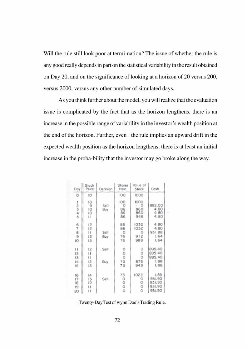
To illustrate, on Day 2, the investor sells his 100 shares at a price $9;

but he must pay a 2% commission, which amounts to (.02 X $9 X 100 =

$18); thus he receives only $882(= $900 - $18) from the sale. On Day 3, he

repurchases the stock Once again he must pay a 2% commission, so

effectively the stock price is $I0.20 a share. Since he has $882 cash, he can

purchase only 86 shares, leaving him $4.30 (= S882 — 86 x 810.20) cash.

Notice that at the end of the 20th day, the investor’s cash position—$931.90-

—is worse following the rule than it would have been if he had sold his 100

shares on Day 0 and thereby re-ceived 8980 cash, after paying the

commis-sion.

Given all the model’s assumptions, is Cherning’s rule profitable?

Probably your immediate reaction is, “No.” But wait a minute. Suppose

instead of arbitrarily select-ing 20 days as the length of the simulation, you

had picked either 6 or 16 days instead. What would your answer have been

then ? Or suppose you rerun the simulation with a new history of 20 tosses.

71

Will the rule still look poor at termi-nation? The issue of whether the rule is

any good really depends in part on the statistical variability in the result obtained

on Day 20, and on the significance of looking at a horizon of 20 versus 200,

versus 2000, versus any other number of simulated days.

As you think further about the model, you will realize that the evaluation

issue is complicated by the fact that as the horizon lengthens, there is an

increase in the possible range of variability in the investor’s wealth position at

the end of the horizon. Further, even ! the rule implies an upward drift in the

expected wealth position as the horizon lengthens, there is at least an initial

increase in the proba-bility that the investor may go broke along the way.

Twenty-Day Test of wynn Doe’s Trading Rule.

72

So as you can see, even this simple-minded simulation gives rise to

some dif-ficult questions concerning what to measure and how to design a

scientific experi-ment to test the effectiveness of the rule. What is more, if

you take the trouble to run the mode) by hand for another 20 periods, you

will quickly appreciate the desirability of letting an electronic computer do all

the coin tossing and arithmetic.

3.4 BUILDING A SIMULATION MODEL

We now return to a more general discussion of the steps involved in

using computer simulation. In this section we examine three aspects of model

building: specifying the model’s components; testing its validity and reliability;

determin-ing its parameters and measuring its performance,

Model components. The structure of most simulation models is

con-veniently described in terms of its dynamic phenomena and its entities.

The dynamic phenomena in the stock market simulation of the preceding

section include the investor’s activity of buying or selling the stock, according

to the stated decision rule, and the factors governing the movement of stock

prices. The entities on any day include the amount of stock the investor

holds, his cash posi-tion, and wealth. Typically, the entities in a model have

attributes. To il-lustrate, the amount of stock the investor holds has a monetary

value, given the associated price of the stock. Further, there are membership

relationships providing connections between the entities. For example, the

investor’s wealth on any day includes both his cash and stock positions.

73

At any instant of a simulation, the model is in a particular state. The

descrip-tion of the state not only embodies the current status of the entities

but frequently includes some historical information. For example, the state of

the system at the beginning of a day in the stock market simulation is described

by yesterday’s price, how yesterday’s price differed from the price on the

day before, the number of shares held, and the cash position.

A model also can encompass exogenous events, that is, changes that

are not brought about by the previous history of the simulation. To illustrate,

the investor in the stock market simulation may have decided to add $1000

more cash from his savings on Day 21, regardless of how well he has done

using the tested strategy.

Knowing the state of the system and the dynamic phenomena, you can

then go on to determine the subsequent activities and states. Frequently,

simulation models having this evolutionary structure are called recursive or

causal.

Note that in building a causal model, you must resolve the way activities

occur within a period. For example, on each day of the stock market simulation,

first the price is determined, then the decision to buy or sell is exercised.

Actually, the price of a stock may change several times during a day, so the

model we con-structed is only a rough approximation to reality. The mode!

also assumes that if the investor sells the stock, he receives the cash at the

end of the day; and anal-ogously, if he purchases the stock, he pays the cash

at the end of the day. Such financial transactions do not always occur so

74

rapidly in practice.

Model validity and reliability. After building a simulation model,

you are bound to be asked, “How realistic is it?” The more pertinent question

is, “Does the model yield valid insights and reliable conclusions?” After all,

since the model can only approximate reality, it must be evaluated by its

power to analyze the particular managerial decisions you are studying.

Once the purpose of the simulation experiment is defined, you construct

each piece of the model with a commensurate amount of detail and accuracy.

A caveat is in order here. As simulation experts can attest, it is easy For a

novice to build a model that, component by component, resembles reality;

yet when the pieces are hooked together, the model may not behave like

reality. So beware not to assume blindly that the entire simulated system is

sufficiently accurate, merely because each of the component parts seems

adequate when considered in isolation. This warning is especially important,

because usually the objective of a simulation model is to fathom the behavior

of a total system, and not that of the separate parts.

Model parameters and performance measures. It is one thing to

describe the pieces of a simulation model abstractly, and it is another to

collect sufficient data for a trustworthy representation of these pieces. Limited

availa-bility of data may very well influence the way you build a simulation.

You must be particularly cautious when you are dealing with extrapolated

75

data and nonstationary performance measures. (Remember the story of the

cracker barrel manufacturer who, not so very long ago, forecasted that he

would be selling millions of barrels today. He assumed, unquestioningly, that

his sales trend would continue as it had in the past.)

You also must watch out for cyclical or periodic phenomena, When

these are present, you must be judicious in selecting the variables to measure

in the experi-ments. If you look only at “ending values,” for example, then

your conclusions may be very sensitive to the exact length of the horizon that

you simulated.

3.5 GENERATING RANDOM PHENOMENA

Most applications of simulation models encompass random

phenomena. For example, in simulated waiting line models, the random

variables include arrival and service times; in inventory models, the variables

include customer demand and delivery times; and in research and development

models, the variables include events of new product discoveries. Frequently,

such simulations require thousands, and sometimes hundreds of thousands,

of draws from the probability distributions contained in the model. How an

electronic computer makes these draws is the subject of this section.

Uniform random numbers. As you will see, the basic building block

for simulating complex random phenomena is the generation of random digits.

The following experimental situation is an illuminating description of what we

76

mean by generating a sequence of uniform random numbers,

Suppose you take ten squares of paper, number (hem 0, 1, 2, . . . , 9,

and place them in a hat. Shake the hat and thoroughly mix the slips of paper.

Without looking, select a slip; then record the number that is on it. Replace

the square and, over and over, repeat this procedure. The resultant record of

digits is a particular realized sequence of uniform random numbers. Assuming

the squares of paper do not become creased or frayed, and that you thoroughly

mix the slips before every draw, the nth digit of the sequence has an equal, or

uniform, chance of being any of the digits 0, 1, 2, . . . , 9, irrespective of all

the preceding digits in the recorded sequence.

In a simulation, you typically use random numbers that are pure

decimals.So, for example, if you need such numbers with four decimal places,

then youcan take four at a time from the recorded sequence of random digits,

and placea decimal point in front of each group of four. To illustrate, if the

sequence of digits is 3, 5, 8, 0, 8, 3, 4, 2, 9, 2, 6, 1, . . . , then the four-

decimal-place random numbers are .3580, .8342, .9261, Suppose you have

to devise a way for making available inside a computer a sequence of several

hundred thousand random numbers.You would probably first suggest this

idea; perform something like the “slips-in-a-hat experiment”

described above, and then store the recorded sequence in the computer’s

memory. This is a good suggestion, and it is sometimes employed. The

RAND Corporation, using specially designed electronic equipment to perform

the experiment, actually did generate a table of a million random digits. The

77

table can be obtained on magnetic tape, so that blocks of the numbers can be

read into the high-speed memory of a computer as they are needed. Several

years ago, this tabular approach looked disadvantageous, because

considerable computer time was expended in the delays of reading numbers

into memory from a tape drive. But with recent advances in computer

technology and programming skill, these delays have been virtually eliminated.

Experts in computer science have devised mathematical processes for

generating digits that yield sequences satisfying many of the statistical

properties of a truly random process. To illustrate, if you examine a long

sequence of digits produced by these deterministic formulas, each digit will

occur with nearly the same frequency, odd numbers will be followed by even

numbers about as often as by odd numbers, different pairs of numbers occur

with nearly the same frequency, etc. Since such a process is not really random,

it is dubbed a pseudo-random number generator.

Computer simulation languages, like those discussed in Sec. 21.8,

invariably have a built-in pseudo-random number generator. Hence, you will

rarely, if ever, need to know specific formulas for these generators. But if you

want to strengthen your confidence in the process of obtaining the numbers,

then you can study the example of a pseudo-random number generator given

below. If not, go on to the discussion of how to generate random variables.

Congruential method. To begin, we need to review the idea of

modulus arithmetic. We say that two numbers x zndy are congruent,modulo

m, if the quantity (x — j) is an integral multiple of m. For example,

78

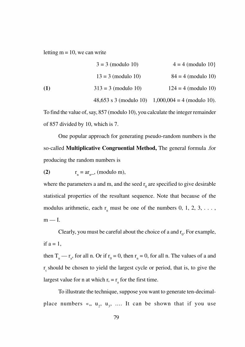
letting m = 10, we can write

3 = 3 (modulo 10) 4 = 4 (modulo 10}

13 = 3 (modulo 10) 84 = 4 (modulo 10)

(1) 313 = 3 (modulo 10) 124 = 4 (modulo 10)

48,653 s 3 (modulo 10) 1,000,004 = 4 (modulo 10).

To find the value of, say, 857 (modulo 10), you calculate the integer remainder

of 857 divided by 10, which is 7.

One popular approach for generating pseudo-random numbers is the

so-called Multiplicative Congruential Method, The general formula .for

producing the random numbers is

(2) rn = arn_, (modulo m),

where the parameters a and m, and the seed r0 are specified to give desirable

statistical properties of the resultant sequence. Note that because of the

modulus arithmetic, each rn must be one of the numbers 0, 1, 2, 3, . . . ,

m — I.

Clearly, you must be careful about the choice of a and r0. For example,

if a = 1,

then Tn — ra, for all n. Or if r0 = 0, then rn = 0, for all n. The values of a and

rc should be chosen to yield the largest cycle or period, that is, to give the

largest value for n at which r, = ra for the first time.

To illustrate the technique, suppose you want to generate ten-decimal-

place numbers «„ u2, u3, .... It can be shown that if you use

79

ua — ra x 10 ~10, where

(3) rn = 100,003 rn_, (modulo 101Ch)

r0 = any odd number not divisible by 5,

then the period of the sequence will be 5 X 10a; that is, ra = r0 for the first time

at n = 5 X 10s, and the cycle subsequently repeats itself. Given that you want

ten-decimal-pi ace numbers, this is the maximum possible length of period

using (2). (There are other values for a that also give this maximum period.)

Verify that the selection of ra in (3) eliminates the possibility that rn — 0; so un

satisfies 0 < u» < 1.

Let us look at an example of (3). Suppose r0 ~ 123,456,789. Then

(4) r, = (100,003).(123,456,789) = 12,346,049,270,367

= 6,049,270,367 (modulo 10’”),

so that u, = .6049270367, and

(5) ra = (100,003) - (6,049,270,367) = 604,945,184,511,101

= 5,184,511,101 (modulo 1010),

80

so that u2 = . 5184511101. The decimals um,n

= 1, 2, . . . , 20, are shown in Fig. 21.5. Notice

that the rightmost digits in this sequence form

a short cycle 7, 1, 3, 9, 7, I, 3, 9, .... Thus the

statistical properties of the digits near the end

of the number are far from random.

While (2) works reasonably well for

some types of simulation models, it has poor

serial correlation proper-ties that make it

dangerous to use for dynamic systems. A

simple device for rectifying this deficiency is

to intermix several sequences, each being

generated with a different value for the seed ?0,

and possibly a different value for a. For

example, you can sequentially rotate among,

say, 10 of these generators.

The advantage of using a pseudo-

random number generator in lieu of a recorded

table of random numbers is that only a few

simple computer instructions are required to

generate the sequence. Therefore, the approach

uses only a small amount of memory space

and does not require reading magnetic tape.

n Un

1 .60492 70367

2 .51845 1 1 101

3 .66636 33303

4 .332 1 1 99909

5 .99544 99727

6 .9836 1 99181

7 .94266 97543

8 .80343 92629

9 .33660 77887

10 .78869 33661

II .70269 00983

12 .1 1790 02949

13 .383 1 9 08847

14 .23804 26541

15 .97953 79623

16 .73484 38869

17 .59322 16607

18 .94573 49821

19 .33541 49463

20 .50087 46389

The Multi-plicative

Congruential Method: a =

100,003; TO = 123,456,789.

81

Generating random variables. We turn next to an explanation of

how to employ a sequence of uniform random numbers to generate complex

proba-bilistic phenomena. The treatment below suggests several techniques

that can be used; but it is by no means exhaustive. Further, the examples that

illustrate the techniques are chosen more for expository ease than

computational efficiency. In an actual situation, you should seek the advice

of a computer science specialist to determine the appropriate technique for

your model.

Inverse Transform. Method. The following is the simplest and most

fundamental technique for simulating random draws from an arbitrary single-

variable probability distribution. Let the distribution function for the random

variable be denoted by

F(x) = probability that the random variable has a value less than or

equal to x.

For example, suppose the random phenomenon has an exponential density

function

(6) f (t) = λe-λτ, τ ≥ 0,

then x

(7) F (x) 0 λe-λτ dt = 1 - λe-λx

Now 0 <F(x) < I, and suppose F(x} is continuous and strictly

increasing. Then given a value ut where 0 < a < 1, there is a unique value for x

such that F(x) = u. Symbolically, this value of x is denoted by the inverse

82

functionF-1(u}. The technique is to generate a sequence of uniform random

decimal numbers Un, n = 1, 2, . . . , and from these, determine the associated

values as xn = F-1(un).

The correctness of this approach can be seen as follows. Consider

any two numbers aa and a6, where 0 < aB < u6 < 1 . Then the probability that

a uniform random decimal number u lie’s in the interval ua <C u < w6 is a0 —

ua. Since F(x) is continuous and strictly increasing, there is a number xa such

that F(xa) — ua, and a number x& such that F(xb) = u6, where xa < xb. The

Inverse Transform Method is valid provided that the true probability of the

random Variable having a value between xa and xb equals the generated

probability ub — ua. This true probability isF(xb) — F(xa) = ub — ua by

construction, so that the method is indeed valid.

To see how this method works, return to the exponential distribution (6) and

(7). Let VT, denote a uniform random decimal number. Set

(8) vn = 1 - e-λxn ,

so that

(9) xn = -loge (1- vn) = -loge un

λ λ

where un = 1 — vHt and hence is itself a uniform random decimal number.

Thus, you generate a sequence of uniform random decimal numbers u1, u2,

u3. . . . , and by (9) compute xt, x2, x3, . . , , to obtain a random exponentially

distributed variable. A diagrammatic representation of the technique is shown

83

The idea can also be applied to a probability mass function P(j), Suppose j =

0, 1,2, 3,..., so that

x

(10) F (x) = ∑ p(j)

J=0

hen the inverse function can be written as

(11) xn = j for F (j – 1) < un ≤ F (j),

where we let F( — l) = 0. For example, suppose the probability mass function

is the binomial distribution:

(12) p(j) = (k)pj (1 – p)k-j for j = 0, 1, ……, k,

j

where 0 < p < 1, and k is a positive integer. In particular, assume k = 2 and p

=.5; thenp(0) = 1/4,p(1)1/2 and p(2)=1/4, so that by (11) you have

(0 for 0 < K» < .25

0 for 0 < un ≤ .25

84

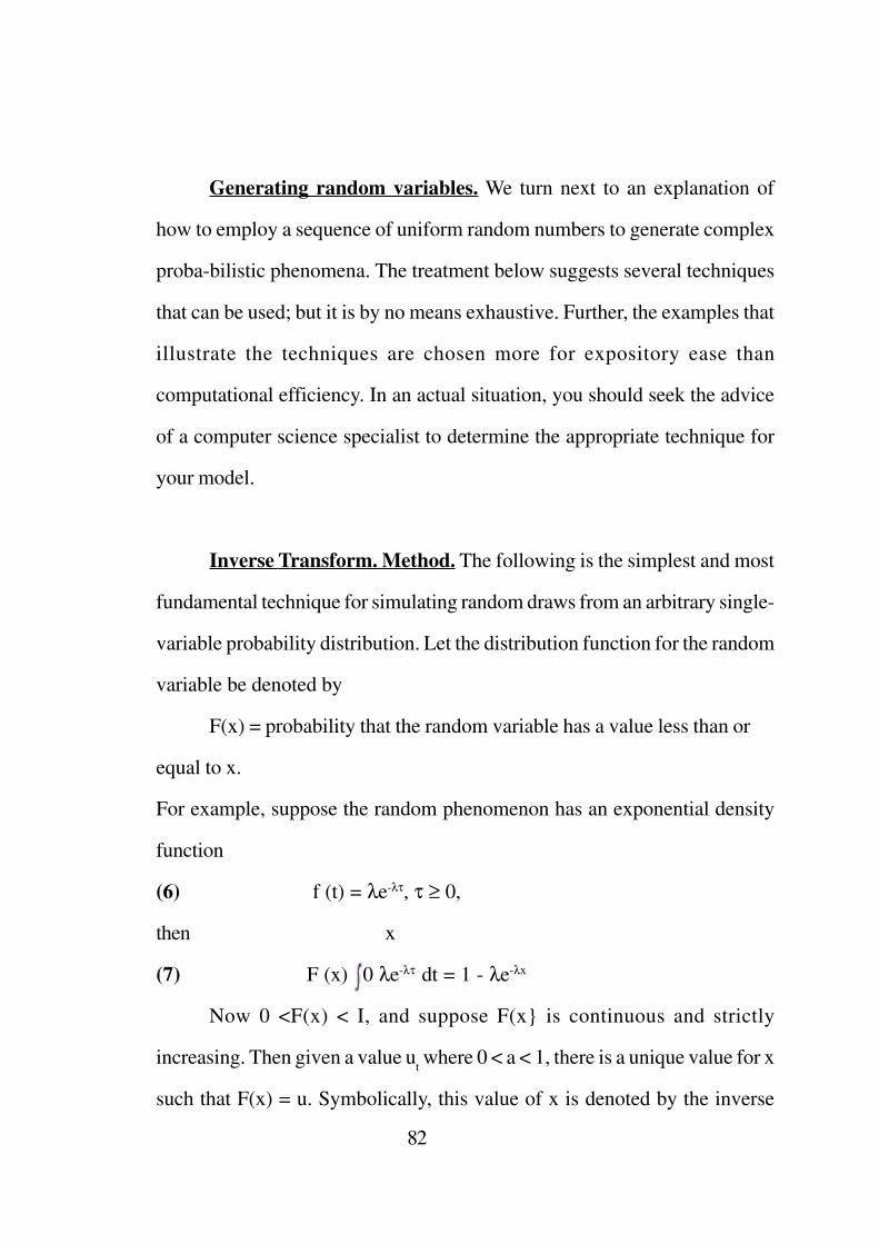
(13) xn = 1 for .25 < un ≤ .75

2 for .75 < un ≤ 1.

Since un, is a uniform random decimal number, there is a 1/4 probability that

un lies between 0 and .25, a 1/4 probability that it lies between .25 and .75)

and a £ probability that it lies between .75 and 1. A diagrammatic representation

of the technique is shown Of course, many continuous distribution functions

F(x} do not have analytic inverse functions as cioes the exponential

distribution. The Inverse Transform Method can still be applied in these

instances by employing a discrete approxima-tion to the continuous function,

that is, by storing the values of F(x) for only a finite set of x. The accuracy of

the approximation can be improved by interpolating between the stored values.

In several computer simulation languages (such as GPSS), you need only

specify this discrete approximation, and the corresponding random

phenomenon will be automatically generated.

85

Tabular Method. The rule in (II) is easily implemented for an electronic

computer by means of a few standard programming instructions. But if the

range of possible values for j is large, then an excessive amount of time may

be consumed in searching for they that satisfies the inequalities in (11). A

faster version of the Inverse Transform Method can be employed at the

expense of using part of the computer’s internal memory for storing a long

table. We illustrate the idea with the binomial example (13).

You can store the inverse function in computer memory in the form

0 for s = 1, 2, …, 25,

(14) G(s) = 1 for s = 26,27, … 75,

2 for s = 76,77,… 100.

Given a value of uni let da be the number formed from the first two digits of

un. Set sn = da + I, and let xn = G(fn). For example if ua = .52896. . . , then sn

= 52 + 1 = 53, and so *„ = G(53) = I in (14). Once the function G(s) has

been stored in memory, only a few calculations must be performed by the

com-puter to produce XN.

Method of Convolutions. Sometimes you can view a random variable

as the sum of other independently distributed random variables. .When this

is so, the probability distribution of the random variable is a convolution of

probability distributions, which may be easy to generate. (Occasionally, you

can obtain a workable approximation to a complex probability distribution

by using a weighted sum of independently distributed random, variables. For

86

this reason, the approach aiso has been called the Method of Composition.)

To illustrate, consider a random variable having a gamma density function

(15) g(y) = λ(λy)k-1e-λv , y ≥ 0, k a positive integer,

(k – 1)!

Such a variable can be considered as the sum of k independent random

variables, each drawn from the same exponential density specified in (6).

Consequently, adding k independent values of x„, as given by (9), yields a

random variable with the distribution in (15).

Similarly, a binomial random variable, as specified in (12), can be

viewed as the sum of k draws of a variable described by

(16) i = 1 with probability p

0 with probability 1 – p.

You can therefore obtain a binomially distributed variable by adding k

values of i. Each of these values for i is determined by the rule

(17) i = 1 for 0 < u ≤ p

0 for p < u ≤ 1,

where u is a uniform random decimal number.

Method of Equivalent Transformations. Sometimes you can

generate a random variable by exploiting a correspondence between its

probability distribution and that of a related random variable.

For example, consider the Poisson distribution written in the form

87

(18)(18)(18)(18)(18) p(j) = (λΤ)je-λΤ for 0, 1, 2, …,

J!

which has mean λT. In terms of the waiting line models you can interpret j as

the number of customers arriving during a period of length T, where the

interarrival times for the customers are independently and identically dis-tributed

exponential random variables with the density function specified in (6).

Consequently, you can generate a Poisson distributed random variable by

making successive independent draws of an exponentially distributed variable

— using (9) to obtain such values. You stop making draws as soon as the

sum of j + 1 of these variables exceeds T. The distribution of the resultant j is

(18) Explain why.

Normally distributed random variables. Unfortunately, the

distribution function for the Normal density with mean 0 and variance 1,

(19) F(x) = 1 e-t2/2 dt,

-∞ 2Π

does not yield an analytic formula for the inverse function F-1(a). Of course

the Inverse Transform Method can be used by employing a discrete

approximation, and interpolating between values. But there are other methods

for generating a Normally distributed random variable. Only a few are

presented here.

One technique requires generating a pair of independent uniform random

decimal numbers u and v, and in turn yields a pair of independently distributed

88

Normal random variables x and y having the distribution function in (19).

Specifically, compute

(20) x = (-2 loge u)1/2 cos 2Πv

y = (-2 loge u)1/2 sin 2Πv

Alternatively, you can apply the Method of Convolutions and invoke the

Central Limit Theorem. This technique employs the sum of k independently

and identically distributed uniform random variables. Specifically, let uit for i

= 1, 2, . . . , 12, be independent draws of a uniform random decimal number;

then compute

12

(21) x = ∑ ui – 6

i-1

The distribution of x will have mean 0 and variance 1, and will be approximately

Normal. The approximation is poor for values beyond three standard

deviations from the mean.

A third approach is to compute

(22) x = [ (1 – u)-1/6.158 – 1] -1/4.874 – [u-1/6.158 – 1]-1/4.874

.323968

where u is a uniform random decimal number.

Correlated random variables. There are straightforward ways to

generate variables from a multivariate Normal distribution, and from other

joint probability distributions, as well as random variables having serial

89

correla-tion. The techniques go beyond the scope of this book, but can be

found in most texts on computer simulation.

3.6 HOW TO MARK TIME

A dynamic systems simulation model can be structured in either of

two ways. One approach, which is the more obvious, views simuiated time

as elapsing period by period. The computer routine performs all the

transactions taking place in Period t, and then proceeds to Period t -j- 1. If

the events in Period t imply that certain other transactions are to occur in

future periods, then the computer stores this information in memory, and

recovers it when the future periods arrive. You already saw an illustration of

this approach using fixed-time increments in the stock market simulation of

Sec. 21.4. Another example is given below.

In some simulations, the periods have to be relatively short. But there

may be many of these periods in which no transactions occur. For such

models, there is a second approach that lets the simulation advance by variable-

time incre-ments. This idea is illustrated in the second example below.

Time-step incrementation — inventory model. Suppose you wish

to evaluate the operating characteristics of a proposed inventory replenish-ment

rule. Assume that you can specify the probability distribution for each day’s

demand, and that daily demand is identically and independently distributed.

If demand exceeds the amount of inventory on hand, the excess represents

90

lost sales. Let us postulate that, during a daily time period of the simulation

model, the sequence of events is: first, any replenishment order due in arrives;

then demand occurs; and finally, the inventory position is reviewed, and a

reorder is placed if the replenishment rule indicates it should be. An order

placed at the end of Period t arrives at the start of Period t + L, where L is

fixed and L > 1.

To keep the exposition simple, assume that the replenishment rule is to

order Q units whenever the amount of inventory on hand plus inventory due

in is less than or equal to s, where Q > s. Verify that the inequality Q > s

implies there is never more than one replenishment order outstanding. (Since

our focus here is simulation and not inventory theory, we do not comment

further on the rea-sonableness of the replenishment rule; we do point out,

however, that the model is an approximation to that in Sec. 19,6.)

A simulation model of this inventory system is easily constructed by

stepping time forward in the fixed increment of a day, beginning with Day 1

(f — I). To start the simulation, you must specify the initial conditions of the

level of inventory on hand, the amount due in, and the associated time due in.

You must also designate the number of periods that the simulation is to run;

let the symbol “HORIZON” denote this value.

A flow chart of the simulation is shown in Fig. 21.8. The initializing is

done in Block 1. For example, you can lei the amount INVENTORY ON-

HAND = Q,, the AMOUNT DUE-IN = 0, the TIME DUE-IN = 0, and t = 1.

Verify that when Block 2 is reached, the answer is “No,” and you proceed at

91

Block 4 to generate a value of demand q for Day 1. Here is where you use an

approach from the preceding section.

At the end of Day 1, INVENTORY ON-HAND is diminished by q,

unless q exceeds the amount available, in which case the amount

of-INVENTORY ON-HAND becomes 0. This calculation is performed at

Block 5.

At Block 6, a test is made to determine whether a replenishment order

is to be placed. If so, the AMOUNT DUE-IN becomes Q., and the TIME

DUE-IN becomes I + L(since at the start t = 1), as indicated in Block 7. If a

replenish-ment order is not placed, you continue directly to Block 8, where

the time step is incremented by 1; that is, the simulation clock is advanced to

Day 2.

If Day 2 goes beyond the HORIZON you specified, the simulation

terminates. Assuming that you set the HORIZON > 1, the simulation returns

from Block 9 to Block 2.

At some day, TIME DUE-IN will equal (, and then the simulation

branches from Block 2 to Block 3, where the amount of INVENTORY ON-

HAND is augmented by Q, and the AMOUNT DUE-IN is reset to 0.

The flow chart does not indicate where you would collect statistical

data on the operating characteristics of the system. In programming the model,

you would keep a tally at Block 5 of the level of INVENTORY ON-HAND at

the end of a day, as well as of the amount of lost sales and the number of

days when a stockout occurs. You would tabulate at Block 6 the number of

92

days an order was placed.

Then, before terminating the simulation at Block 10, you would summarize

these tallies into frequency distributions, along with their means, standard

deviations, and other statistical quantities of interest.

Suppose the item is a “slow mover,” that is, there is a high probability that

demand q = 0 on any day. Then the time-step method may be inefficient,

because there will be many consecutive days when the computations in Blocks

2, 5, and 6 will be identical. Such redundancies can be eliminated by using

93

the technique illustrated below.

Event-step incrementation—waiting line model. Suppose you want

to examine the operating characteristics of the following queuing sys-tem,

which is simple to describe but proves difficult to analyze mathematically.

Customers arrive at the system according to a specified probability distribution

for intcrarrival times. The system has two clerks, A and B. When both servers

arc busy, arriving customers wait in a single line and are processed by a first

come, first served discipline. The service times for each clerk can be viewed

as indepen-dent draws from a specified probability distribution; but each

clerk has a different service time distribution. Neither the imerarrival nor the

service time distributions are exponential.

After thinking about the way this system evolves over time, you will

discover that the dynamics can be characterized by three types of events: a

customer’s arrival, a customer’s service begins, and a customer’s service

ends. Each event gives rise to a subroutine in the computerized version of the

system,

A simulation model using variable-time increments also contains a

master program having an event list, which is repeatedly updated as the

master program switches from one event subroutine to another. At the start

of a simulation run, the event list is usually empty; but at a later instant in the

run, it indicates when some of the future events are to occur. The role this

event list plays will be clearer as you examine the event flow charts

94

Assume that you specify the initial conditions of the simulation as: a

customer arrives, say, at Time 0, there are no customers in line, and both the

clerks are free. The master program starts with the event subroutine

CUSTOMER AR-RIVES, shown as Block 1 in Fir. interarrival time at Block

2. The informa-tion that this next arrival event occurs at the implied future

time is entered into the event list. A determination of whether both clerks are

busy is made in Block 3. Since the answer is “No” at the start, the master

program switches to the event subroutine SERVICE BEGINS, as indicated

in Block 4. To keep the flow diagram uncluttered, we have suppressed the

details that would specify that the computer must keep track of which clerk

serves the customer, an item of information that is needed when the master

program switches to the subroutine SERVICE BEGINS in Block 7.

95

The first instruction in SERVICE BEGINS is at Block 8, which records

that the selected clerk is now busy. Then the service time of the customer is

determined in Block 9, using the appropriate service time probability

distribution for the selected clerk. The information that a service-ends event

occurs at the implied future time is entered into the event list. The subroutine

then transfers back to the master program with the instruction in Block 10 to

find the next imminent event in the event list. So far, this can be either the

arrival of the next customer or the completion of service of the first customer.

Suppose it is the latter, so that the master program switches to the subroutine

SERVICE ENDS in Block 11.

The first instruction in SERVICE ENDS is at Block 12, which records

that the server is now free again. Then a test is made at Block 13 to see

whether the waiting line designated by the symbol “LINE” is empty. Verify

that the answer is “Yes.” Also check that when control switches back in

Block 14 to the master program, the next imminent event will be the arrival of

the second customer.

Later in the run, the LINE will contain customers, and then the answer

is “No” at Block 13. As a result, the length of the LINE is decreased by 1 in

Block 15, and control transfers in Block 16 to the subroutine SERVICE

BEGINS. Explain what can happen subsequently if Block 10 leads to the

CUSTOMER ARRIVES subroutine.

A simulation run progresses as each event subroutine either switches

to another event subroutine or instructs the master program to increment

96

time to the next imminent event. As you can imagine, considerable skill is

required to write a simulation program that uses event-step incrementation.

In particular, expertise is needed to program the updating of the event list

efficiently as future events are generated by the subroutines. Many simulation

languages of the type discussed in Sec. 21.8 already include a master program

that maintains an updated list of events; to employ these languages, you only

have to specify the separate event subroutines.

We have glossed over a number of details in describing the queuing

simulation model. We briefly mention a few of these before going on to the

next section, which considers the design of simulation experiments. First,

note that the charts do not show a test for terminating a simulation run. Of

course, you must include s.uch a calculation; you might state it by means of

a time horizon or limit on the number of customers arriving. Second, observe

that tabulating statistics on the operating characteristics is not an easy process

because of the variable-time increments between successive events. Care

must be taken to mea-sure, for example, not only the frequency with which

the waiting line has n customers, but also the associated fraction of the

simulated horizon. Finally, recall that the initial conditions were chosen

arbitrarily. If the queuing system in fact tends to be congested, then the effect

of letting LINE = 0 at the start will take a while to wear off. Specifying

appropriate initial conditions is part of the tactics of designing a simulation

experiment.

97

3.7 DESIGN OF SIMULATION EXPERIMENTS

After constructing a simulation model, you face the difficult task of

designing a set of runs of the model and analyzing data that emanate from

these runs. For example, you must decide the

• Starting conditions of the model.

• Parameter settings to expose different system responses.

• Length of each run (the number of simulated time periods and the of

amount of elapsed computer time).

• Number of runs with the same parameter settings.

• Variables to measure and how to measure them.

If you are not careful, you can expend an enormous amount of computer

time in validating the model to see whether it behaves like a real system, in

estimating the system responses of the model to different parameter settings,

and in discover-ing the response relationships among these parameters. Even

then, and even after collecting a vast amount of data, you still may not have

sufficiently accurate infor-mation to guide a managerial decision.

Surprising as it may seem, there has been relatively little development

of statistical techniques aimed at constructing efficient designs of simulation

experi-ments. By and large, professional management scientists have tried to

“make do” with standard statistical tools to analyze experimental data from

simulations. These techniques at best are only moderately successful, because

most of them are not constructed for the analysis of multidimensional time

series data. In particular, many (but not all) of the commonly used statistical

98

tools assume that separate observations of the variables being measured are

uncorrelated and drawn from a Normal distribution with the same parameters.

We cannot possibly summarize all of the standard statistical techniques

that can be applied to analyze simulation data. Instead, we discuss certain

design procedures that enable you to employ many techniques ordinarily

found in a this section requires a. knowledge of statistical methods modern

text on experimental statistics. We also give a brief a statistical approaches

that are particularly well suited to the simulations.

In search of Normality, Suppose you have constructed a queuing

model to test two different service disciplines. For example, your application

may-be a model of a job-shop production system, and the two disciplines

lor processing orders are “first come, first served” and a particular priority

scheme. Assume further that the difference in the two disciplines is to be

measured solely in terms of the average waiting lime (exclusive of service)

for orders. How might you ascertain what this difference is ?

This question is more difficult than it may appear at first glance. Since

your measurements will be random variables, you must consider their statistical

variability and be on the watch for certain kinds of complications. In any

single simulation run, the waiting times of successive orders will be serially

cor-related (sometimes called autocorrelated) ; that is, there is a greater

like-lihood thai ihe (n + l)st order will be delayed if the nth order waits, than if

the nth order commences service immediately. The extent of variation in

99

waiting times may itself be affected by the two different disciplines. The

model may be unstable and the trend of waiting times may be ever upward.

Even if the system does approach equilibrium, which may require a

considerably long run, wailing limes need not be Normally disiributed. To

ignore all these considerations and simply compare the average wailing times

from a simulated run of each discipline is to court disaster.

Suppose you can demonstrate, on theoretical grounds, that ihe queuing

model is stable, and thai the effects of the starting conditions eventually fade

away. Then it can be proved that even though the waiting times of successive

orders are autocorrelated, the expected value of the sample average of these

waiting times, taken over a sufficiently long run, is approximately that implied

by the equilibrium distribution.

More precisely, let *,, for i — 1,2, . . . , q, represent q successive data

observa-tions of ihe random variable in a given simulation run, and define the

time-integrated average as

q

(1) x = ∑ xt .

t=1

Let u represent the so-called ensemble mean of this random variable, as

calculated from the equilibrium distribution. Then for q sufficiently large, we

have the approximation

(2) E[x] ≈ µ

Furthermore-, il can be shown that the sampling distribution of x is

100

approx-imately Normal. You can calculate an estimate of the variance of this

dish ibuiion as follows. Assuming that the process is covariance-stationary

(the covariance between xt and xt+k depends only on k and not on t), and that

the associated autocorrelations tend to 0 as k grows large, you first estimate

these autocorrelations by :

q-k

(3) rk = 1 ∑ (xt+k – x) for k = 0, 1, 2, …, M,

q-k t=1

where M is chosen to be much smaller than q. (Unfortunately, a discussion

of how much smaller M should be is too complicated to be given here, but

can be found in the statistics literature under the subject title autocorrelation

and spectral analysis.) The appropriate estimate of the variance of x is

M

(4) Vx = 1 r0 + 2 ∑ (1 – k/M)rk

K=1

Note that if, in fact, the time series is known to be free of autocorrelation,

then the terms rt, for k = 1,2,..., M, would be eliminated from (4). The presence

of positive autocorrelation, however, implies greater statistical variability in x

as compared with the case of uncorrelated observations.

We now can look at two commonly employed approaches to statistical

analyses. For the first method, consider making one very long run of each

service discipline; specifically, take T consecutive observations in each run.

Then you can apply (1) through (4) with q = T. If T is sufficiently large, the

101

statistic (x — u)J/vPs is approximately Normally distributed with mean 0 and

variance I. This fact allows you “to perform standard statistical procedures

for hypothesis testing and construct-ing confidence intervals for fj., as well

as to use modern Bayesian analysis. To compare the effect of the two service

disciplines on average waiting time, you can apply standard statistical theory

for discerning -the difference between the means of two Normally distributed

variables that have possibly unequal and estimated variances.

For the second method, consider making ;i independent replications, that is,

n different runs. Suppose you want to have T observations in luta from the n

replications and that you take Tjn observations from each run (assume Tjti is

an integer}. Then for each replication p. calculate a time -integrated average

xv, for p = 1, 2, . . . , n, using (!) with q = T/n. Afterwards compute the grand

average

n

(5) x = ∑ xp

P=1 n

For any T/n, if n is large enough, the sampling distribution of x is approximately

Normal due to the Central Limit Theorem for the mean of independently and

identically distributed random variables (namely, the x0). If you let Tjn be

large enough, the approximation is improved because of the near -Normality

of the sampling distribution for each xt. What is more, it follows from (2) that

when T/n is sufficiently large,

102

(6) E[x] ≈ µ.

To determine the accuracy of x, you can estimate the variance of the

sampling distribution of x from the variation in xp, using

n

(7) Vx = 1 ∑ (xp – x)2

N n – 1

Once again, if n and T are large, the quantity (x — u)/vVj is

approximately Normally distributed with mean 0 and variance 1, and so the

same sorts of sta-tistical analyses can be performed as in the one-long-

replication procedure.

Although the preceding discussion has related to a comparison of two

different service disciplines in a job-shop model, these statistical approaches

are generally applicable. In summary, assuming that the simulated system

does approach an equilibrium, then under widely applicable conditions, you

can legitimately average the successive observations of a simulated time series.

As the number of observa-tions grows large, this time-integrated average, in

a probabilistic sense, converges to the desired ensemble mean implied by the

equilibrium, distribution. (You can find the subject of probabilistic convergence

treated in detail in texts on stochastic processes under the heading ofergodic

theorems.} And furthermore, under widely applicable conditions, the time-

integrated average is approximately Normally distributed. {You can look up

the topic of Normal approximations in advanced statistics texts under the

heading of the Central Limit Theorem for correlated random variables.)

103

Therefore, in many situations you can apply Normal-distribution theory

if you either replicate simulation runs and then take a grand average of the

individual time-integrated averages, or if you take a single time-integrated

average from a very long run. A comparison of the relative merits of these

two approaches as well as of other methods goes beyond the scope of this

text. (The issues involved con-cern ihe amount of bias introduced by the

starting conditions of the simulation and the stability properlies of Vx)

Sample size. Assume that you take a sufficient number of replications

or let the simulation run long enough to justify using the Normal distribution

to approximate the. sampling distribution uf the calculated averages. You still

may need even more replications or a longer run to obtain the accuracy you

require for decision analysis. The determination of an appropriate sample

size for a simula-tion is no different from sample-size determination in ordinary

statistical problems. Therefore, you can find the question discussed in detail

in every text on statistical analysis.

We do emphasize, however, the influence of the number of observations

on the accuracy of the statistical estimates. Whether you use the single-long-

run ap-proach, depicted in (1) through (4), with q = T, or the n-replication

approach, depicted in (5) through (7). with q = T/n. the true variance of the

sampling dis-tribution for the calculated mean equals the reciprocal of the

total number of observations T multiplied by another factor that is independent

of T. Therefore, to reduce the standard deviation of the sampling distribution

104

of either x or 5 from a value of s, say, to (.l)s, you must increase the total

number of observations to

100T. More generally, to reduce the standard deviation by a factor of I//, you

have to take/^ as many observations.

Usually, you cannot know how many observations to take at the start

of a simulation., because you do not know the factors that multiply I/T in the

expres-sions for the true variances of the sampling distributions of x and x.

For this reason, a commonly used procedure is to sample in two stages. In

the first stage, you take a relatively small number of observations, and thereby

calculate an estimate of the factor that multiplies 1/7'. With this estimate, you

determine the remaining number of observations to take in the second stage

to give the required accuracy. In actual applications, you may be surprised to

find how many observations are needed to yield reasonable accuracy in the

estimates. As pointed out above, the root of the difficulty is often the presence

of positive autocorrelation. We discuss below a few approaches for coping

with inherently large variation in the statistical estimates.

Variance-reduction techniques. There are a number of ways to

improve the accuracy of the estimate of the ensemble average for a given

number of data observations. These leehniques arc explained in texts on

simulation under the heading of Monte Carlo or variance-reduction

methods. Their use in management-oriented simulations is not yet widespread.

We give only a couple of illustrations to suggest what is involved.

105

To assist in the exposition, we return to the example above of simulating

a job-shop production system. Suppose, for the sake of definiteness, that

you arc simulat-ing under the “first come, first served” discipline, and that

you want to estimate the average waiting lime of an order.

The first device we examine is sometimes called the Method of

Control Variates, or alternatively, the Method of Concomitant Informa-tion.

W’c present a highly simplified example of the idea. By elementary

consid-erations you know that the interarrival times and the waiting times of

each order are negatively correlated - roughly put, the longer the time since

the previous order arrived, the shorter the waiting time of the latest order.

State why. Therefore, sup-pose in a particular simulation run that the

observed average of interarival times is greater than the true average.Then

you can use this information to add a posi-tive correction to the observed

average value of the waiting times. Similarly, suppose the observed average

of interarrival times is smaller than the true average. Then you can make a

negative correction to the observed average value of the waiting times. The

technique explained below calculates either a positive or negative correction,

whichever is appropriate.

Specifically, from the input data for the simulation you have the value

of the true mean interarrival time, say, 1/X. Then let xt represent the waiting

time of Order t, and^, the mlerarrival time between Orders t — 1 and t.

Consider the measurement

106

(8) zt = xt + yt - 1 ,

λ

and its time-integrated average

T

(9) z = ∑zt = ∑ xt + yt – 1 = x + y – 1

t=1 t=1 λ

Note that the expectation of z is the same as that of x, since y is an unbiased

esti-mator of I/A. So you can use z as a consistent estimate of the average

waiting time. But if xt and yt, are sufficiently negatively correlated, then the

variance of z will be less than the variance of x. A sample estimate of the

variance of z can be calculated by assessing the variation in z from several

replications, or by sub-stituting zt for x, in (I), (3), and (4) above.

A more sophisticated method than (8) is to calculate

z, = xt, + a(yt — l/^)> where now the value of a is specifically chosen to

rnake the variance of z small. Under ideal conditions, a can be set such that

Var (z) = Var (x)(l — p2}, where p is the correlation between x and jr.

Before going on, we caution that the preceding example is meant only

to be illustrative of the control variate idea. If you actually apply the technique

to a queuing model like a job-shop production system, you should select a

control vanate that would absorb more of the sampling variation that would

be accounted for by the inlerarrival times of orders. In fact, you probably

should use several control variates instead of only one.

107

The second variance-reducing device we examine is called the Method

of Antithetic Variates. The aim here is to introduce negative correlation

between two separate replications of the simulation, so that the variance of

the combined averages is less than if the replications were independent. {The

idea can also be extended to more than two replications.)

Suppose in the job-shop production simulation that the interarrival

times are determined by the Inverse Transform Method of Sec.21.5. Let ut,

for t = 1, 2, . . . , TV2, be the corresponding uniform random decimal

numbers for generating the interarrival times yt in the first simulation run of

the model. Then in the second simulation, by using the values 1 — ut, which

are also uniform random decimal numbers, the two time-integrated sample

averages will be negatively correlated. State why.

Notice that the two simulations involve a total of T observations.

Whether the mean of the two separate negatively correlated averages has less

statistical varia-tion than does the average of T autocorrelated observations

from a single run depends on the extent to which the antithetic variates UL and

1 — u, induce nega-tive correlation. Thus, the answer depends on the particular

model being simu-lated, and the specific values of the model’s parameters.

The crucial factor in deciding when to use variance-reduction techniques

is whether, in fact, a given approach diminishes the variance of the estimates,

and if so, whether the reduction is sufficient to warrant the extra computations

re-quired.

108

Multivariate analysis. The discussion so far has been partly

mislead-ing in that we have discussed examples involving the measurement

of only a single operating characteristic for a system, such as average waiting

time, and the comparison of only two alternatives, such as two different

service disciplines. In real applications of simulation models, there are usually

several operating char-acteristics of relevance and a multitude of alternatives

to evaluate.

Multivariate analysis is by no means a new subject in statistics literature,

but techniques for the analysis and design of experiments involving multivariate

time series arc just emerging. The reason for this relatively late development

is that only recently has the availability of electronic computers made it practical

to perform .such data analyses.

By employing the approaches previously described to yield

measurements that are Normally distributed, you have at least partially opened

the storehouse of standard multivariate statistics. But still it is no simple

matter to design a simulation experiment that can legitimately apply, say. latin

squares, factor analysis, or multivariate regression.

Progress in devising helpful tools for multivariate analysis and complex

experi-mentation is being made on two fronts. One important development,

known as spectral analysis, aims at exploring the nature of serial correlation

and periodicities in time series. The other front seeks methods for finding

optimal levels of the decision variables; two such developments are response

surface and stochastic ap-proximation techniques. You can find these

109

developments explained m the technical statistics literature.

3.8 COMPUTER LANGUAGES

Unless you become both an operations research specialist and a

computer-programmer, you personally will not have to translate your simulation

model into a workable computer program. You should, however, know the

major steps involved in this translation.

If your model is fairly simple and is a common application of simulation,

then a so-called canned program may be available in which all you need do

is specify a modest amount of input information. The best examples of this

type of program ;ire inventory control simulators. There are a number of

canned programs that test the effectiveness of inventory replenishment rules.

To employ these routines, you must supply the specific rules, such as “when

down to 4, order 10 more/’ or a formula to calculate the rules, given demand

data. You also supply as part of the input either actual historical data on

customer demand or a proba-bility distribution for demand. The computer

program then simulates the system for whatever number of time periods you

designate, and calculates statistics such as the frequency of stockouts, the

average inventory level, the number of orders placed, etc.

More typically, your model will require some special computer

programming. If the simulation is only moderately complex, is to be used

infrequently, and is to be programmed by personnel inexperienced in simulation

techniques, then using a general purpose language, such as FORTRAN, PL/

110

1; or ALGOL, is probably the easiest way to accomplish the task. This type

of computer language is familiar to all programmers of scientific problems; a

programmer requires only the details of your model to translate it into computer

language.

There is an important drawback to employing languages like

FORTRAN, PL/1, and ALGOL. The programmer has to write, from scratch,

subroutines for certain kinds of calculations that are included in almost all

simulations. In the vernacular, the-programmer has to “reinvent the wheel/’

For example, most simulations require generating random variables, and so a

subroutine is needed for each such variable in the model. In addition, since

you want to collect statistics on the system’s operating characteristics,

subroutines have to be written to calcu-late these statistics, and a fair-sized

associated programming effort must be ac-complished to format the output

of the simulation runs. Even a moderately complex model requires careful

attention in organizing the data within the computer memory, writing a master

routine for sequencing events in their proper order, and keeping track of

simulated time within the computer.

Several computer languages have been developed for the specific purpose

of easing the programming task of building a simulation model. These

programs require that you specify only the probability distribution functions,

and they automatically generate random events according to the distributions

you indi-cate. Several of the languages collect statistics on whatever operating

characteristics you want to examine, and report the results on predesigned

111

output forms. These languages also properly sequence events and keep track

of time as it elapses in the model.

With such advantages, you may wonder why all simulations are not

pro-grammed in one of these languages. At present, there are several good

reasons. One is that the languages differ to some extent from FORTRAN.

PL/I or ALGOL, and hence require a programmer to become familiar with a

new system.

One of the most powerful simulation languages is SIMSGRIPT; it

requires a knowledge of FORTRAN and is fairly complex because of its

considerable flexibility. At the other extreme of complexity is the General

Purpose Systems Simulator (GPSS). It is a self-contained language that is

easy to learn by beginners, but, accordingly, is restricted in its scope.

A second reason for not employing a simulation language is that it may

not be available on the computer you want to use. This is rarely the determining

factor today because SIMSGRIPT and GPSS programs are available for

many com-puters, and there is widespread access to computer service bureaus

that have these programs.

A third reason becomes important if the simulation is complex and is

to be run frequently. A price you pay in using a simulation language is that it

often runs slowly and consumes large amounts of a computer’s high-speed

memory. As a result, you may find it costly to perform many experiments,

and your model may literally not fit into the available memory capacity of the

computer.

112

As further technical improvements in simulation languages continue,

and as management scientists gain more experience in employing computer

simulation, it seems likely that such languages will be the common mode of

solution.

3.9 DEUS EX MACHINA

So far we have discussed only simulation models that to some degree

represent approximations to real situations. Their orientation has been to

provide a simu-lated environment in which to test the effects of different

managerial policies. A related class of simulation models tries to encompass

goal-seeking or purposeful behavior. These models display what is termed

artificial intelligence.

Some of the popular examples of artificial intelligence programs include

computer routines for playing such games as chess and checkers. There also

have been a few applications to managerial problems. One group of

applications focuses on the behaviora. patterns of individual dec is ion-makers.

A measure of 3uch a model’s success is how well it yields decisions agreeing

with those of (the individual whose behavior is allegedly reprcsenled.

Another group of applications deals with complex combinational

problems, like those discussed. 13. They are sometimes referred to as heuristic

programming methods. For example, several of these models have been

designed to derive good schedules for intricate sequencing problems. The

follow-ing illustration suggests how they work.

113

Suppose the goal of the model is lo schedule orders through a job-

shop with maximum equipment efficiency. The computer starts by tentatively

.scheduling a few orders. Tt ihcn selects another order to schedule, and

examines various feasibility restrictions, due dates, and equipment efficiency.

As a consequence, the cf nputer may have to reschedule some of the previous

orders. In brief, the computer model uses, a number of “look-back” and

‘’look-ahead” rules, and pro-ceeds by educated I rial-and-err or toward a

feasible schedule. If the rules are sufficiently sophisticated, then usually the

schedule is good. Frequently, the schedr ule is nearly optimal according to

the specified efficiency criterion, assuming the heuristic rules are promulgated

with reference to this criterion.

Management scientists have also employed computer models for

operational gaming. Some of the early applications, known as management

games, involved several teams of players, each representing a business firm.

A team made decisions about pricing, production quantities, advertising, etc.

The computer served the two-fold purpose of keeping the accounting records,

and of calculating the net impact of the decisions made by the several teams.

More recently, such applications have been used to train personnel in

administrative procedures, and to explore the system dynamics of an industry

in which the competing firms are employing specified strategies.

114