EE 485, Winter 2004, Lih Y. Lin

1

Chapter 3 Beam Optics

- An important paraxial wave solution that satisfies Helmholtz equation is Gaussian beam. Example: Laser.

3.1 The Gaussian Beam A. Complex Amplitude

phase Radial )(2

exp

phase alLongitudin tanexp

factor Amplitude )(

exp)(

)(

2

0

1

2

20

0

−×

−−×

−=

−

zRkj

zzkzj

zWzWWArU

ρ

ρ�

(3.1-7)

2

00 1)(

+=

zzWzW (3.1-8)

+=2

01)(zzzzR (3.1-9)

λ

π 20

0Wz ≡ (3.1-11)

→ Knowing 0W and λ (or 0z ), a Gaussian beam is determined! Ref: Verdeyen, “Laser Electronics,” Chapter 3, Prentice-Hall B. Properties of Gaussian Beam

Intensity and power

EE 485, Winter 2004, Lih Y. Lin

2

−

=)(

2exp)(

),( 2

22

00 zWzW

WIzI ρρ (3.1-12)

( )2002

1 WIP π= (3.1-14)

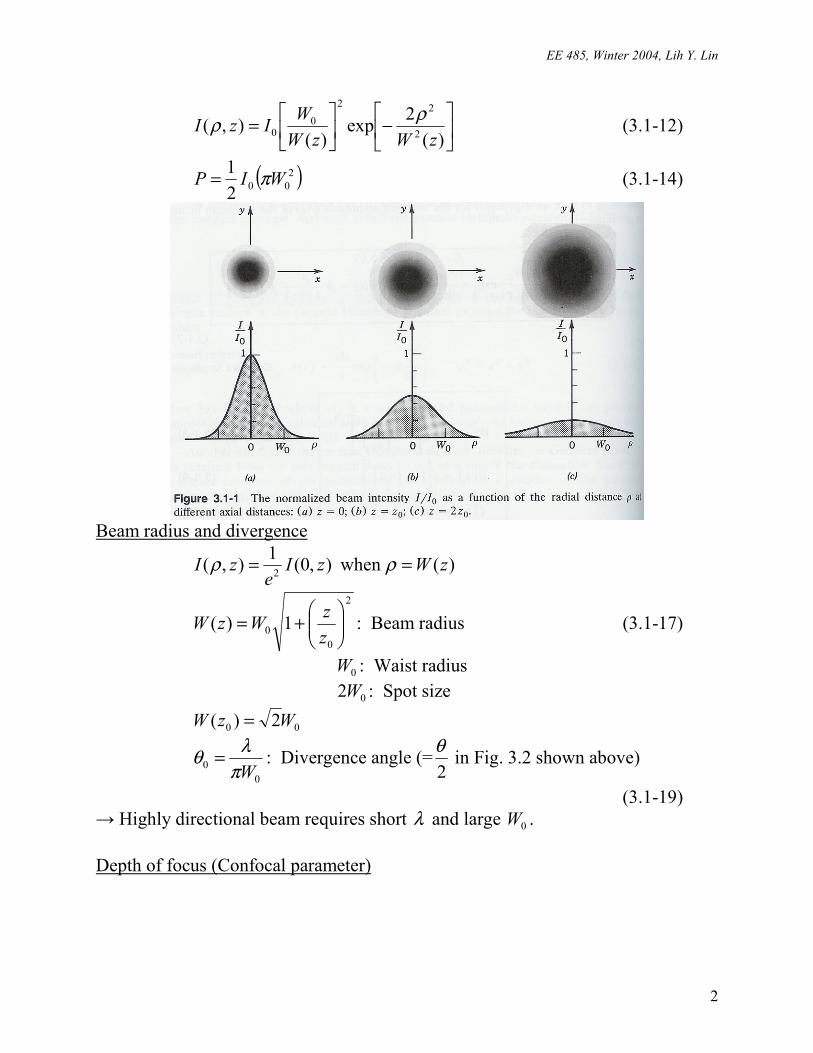
Beam radius and divergence

)( when ),0(1),( 2 zWzIe

zI == ρρ

2

00 1)(

+=

zzWzW : Beam radius (3.1-17)

0W : Waist radius 02W : Spot size 00 2)( WzW =

0

0 Wπλθ = : Divergence angle (=

2θ in Fig. 3.2 shown above)

(3.1-19) → Highly directional beam requires short λ and large 0W . Depth of focus (Confocal parameter)

EE 485, Winter 2004, Lih Y. Lin

3

λ

π 20

022 Wz = (3.1-21)

Longitudinal phase

−= −

0

1tan)(zzkzzϕ

→ Second term: phase retardation

Phase velocity c

zz

z

cz

vp >

−

=

=−

−

0

1

1

tan2

1πλω

ϕ !

Wavefront bending Surface of constant phase velocity:

≡+=+ −

0

12

tan ,22 z

zqR

z ξπλξλρ

→ Parabolic surface with radius of curvature R

EE 485, Winter 2004, Lih Y. Lin

4

3.2 Transmission through Optical Components

Gaussian beam remains a Gaussian beam after transmitting through a set of circularly symmetrical optical components aligned with the beam axis. Only the beam waist and curvature are altered.

A. Transmission through a Thin Lens

WW

RRR=

−=

''

11'

1 (3.2-2)

22

0

'1

'

+

=

RW

WW

λπ

(3.2-3)

EE 485, Winter 2004, Lih Y. Lin

5

2

2

'1

''

+=

WR

Rz

πλ

(3.2-4)

Waist radius 00 ' MWW = (3.2-5) Waist locatioin )()'( 2 fzMfz −=− (3.2-6) Depth of focus )2('2 0

20 zMz = (3.2-7)

Divergence M

00

2'2 θθ = (3.2-8)

Magnification 21 r

MM r

+= (3.2-9)

fz

zrfz

fM r −≡

−≡ 0 , (3.2-9a)

Example: A planar wave transmitting through a thin lens is focused at distance fz =' .

B. Beam Shaping

Waist of incident Gaussian beam is at lens location. fR −='

2

0

00

1

'

+

=

fz

WW (3.2-13)

→ To focus into a small spot, we need large incident beam width, short focal length, short wavelength.

EE 485, Winter 2004, Lih Y. Lin

6

2

0

1

'

+

=

zf

fz (3.2-14)

F number of a lens

DfF ≡#

02WD = : Diameter of the lens

Focal spot size #04'2 FW λπ

= (3.2-17)

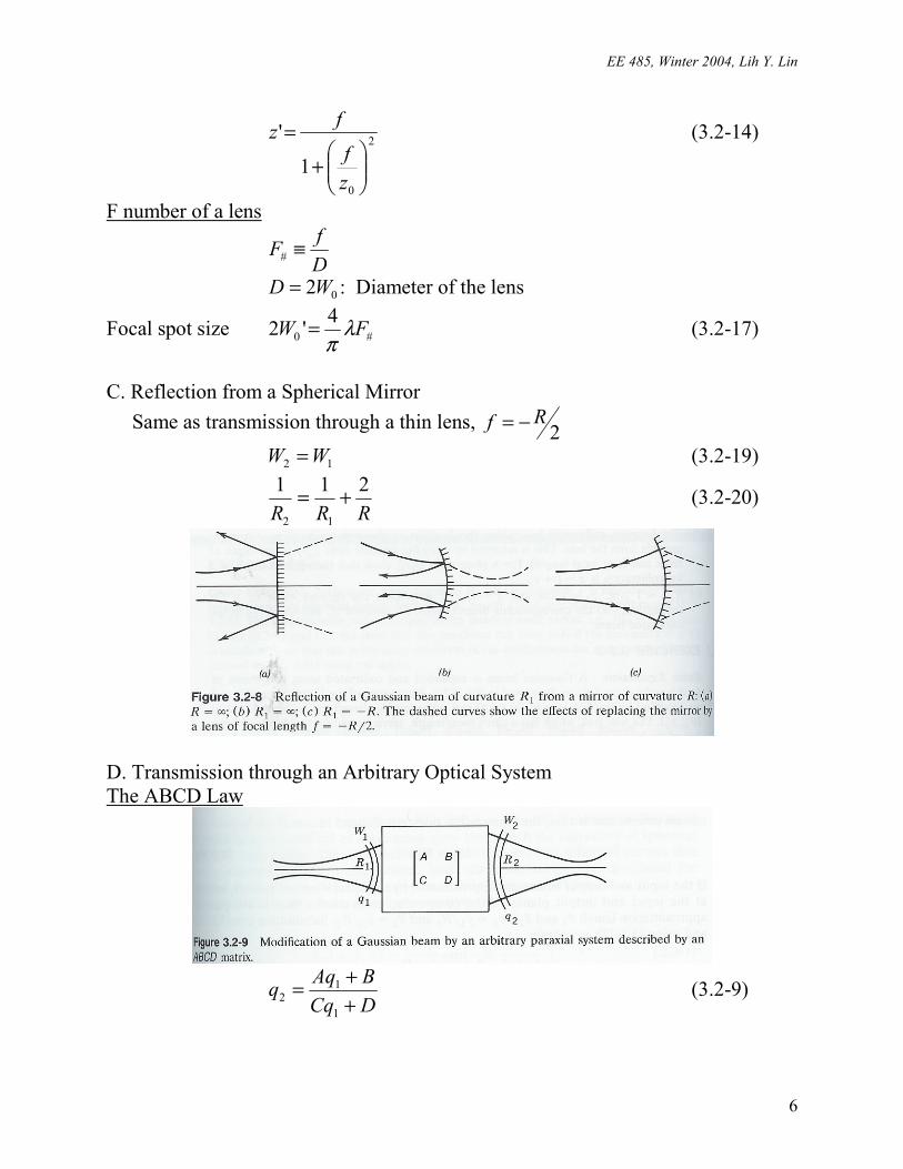
C. Reflection from a Spherical Mirror Same as transmission through a thin lens, 2

Rf −= 12 WW = (3.2-19)

RRR211

12

+= (3.2-20)

D. Transmission through an Arbitrary Optical System The ABCD Law

DCqBAqq

++=

1

12 (3.2-9)

EE 485, Winter 2004, Lih Y. Lin

7

Like in the case of ray-transfer matrix, the ABCD matrix of a cascade of optical components (or systems) is a product of the ABCD matrices of the individual components (or systems). 3.3 Hermite-Gaussian Beams

Modulated version of Gaussian beam → Intensity distribution not Gaussian, but same wavefronts and angular divergence as the Gaussian beam.