Chapter 3 Air Dispersion and Deposition Modeling - Lakes
112
U.S. EPA Region 6 U.S. EPA Multimedia Planning and Permitting Division Office of Solid Waste Center for Combustion Science and Engineering 3-1 Chapter 3 Air Dispersion and Deposition Modeling What’s Covered in Chapter 3: U.S. EPA-Recommended Air Dispersion and Deposition Model Air Model Development Site-Specific Characteristics Required for Air Modeling Use of Unit Emission Rate Partitioning of Emissions Meteorological Data Required for Air Modeling Meteorological Preprocessors and Interface Programs ISCST3 Model Input Files ISCST3 Model Execution Use of Modeled Output Modeling Fugitive Emissions Estimating Media Concentrations Combustion of materials produces residual amounts of pollution that may be released to the environment. Estimation of potential ecological risks associated with these releases requires knowledge of atmospheric pollutant concentrations and annual deposition rates in the areas around the combustion facility at habitat-specific scenario locations. Air concentrations and deposition rates are usually estimated by using air dispersion models. Air dispersion models are mathematical constructs that approximate the physical processes occurring in the atmosphere that directly influence the dispersion of gaseous and particulate emissions from the stack of a combustion unit. These mathematical constructs are coded into computer programs to facilitate the computational process. This chapter provides guidance on the development and use of the standard U.S. EPA air dispersion model that U.S. EPA expects to be used in most situations—the Industrial Source Complex Short-Term
Transcript of Chapter 3 Air Dispersion and Deposition Modeling - Lakes

U.S. EPA Region 6 U.S. EPAMultimedia Planning and Permitting Division Office of Solid WasteCenter for Combustion Science and Engineering 3-1
Chapter 3Air Dispersion and Deposition Modeling
What’s Covered in Chapter 3:
ó U.S. EPA-Recommended Air Dispersion and Deposition Model
ó Air Model Development
ó Site-Specific Characteristics Required for Air Modeling
ó Use of Unit Emission Rate
ó Partitioning of Emissions
ó Meteorological Data Required for Air Modeling
ó Meteorological Preprocessors and Interface Programs
ó ISCST3 Model Input Files
ó ISCST3 Model Execution
ó Use of Modeled Output
ó Modeling Fugitive Emissions
ó Estimating Media Concentrations
Combustion of materials produces residual amounts of pollution that may be released to the environment.
Estimation of potential ecological risks associated with these releases requires knowledge of atmospheric
pollutant concentrations and annual deposition rates in the areas around the combustion facility at
habitat-specific scenario locations. Air concentrations and deposition rates are usually estimated by using
air dispersion models. Air dispersion models are mathematical constructs that approximate the physical
processes occurring in the atmosphere that directly influence the dispersion of gaseous and particulate
emissions from the stack of a combustion unit. These mathematical constructs are coded into computer
programs to facilitate the computational process.
This chapter provides guidance on the development and use of the standard U.S. EPA air dispersion model
that U.S. EPA expects to be used in most situations—the Industrial Source Complex Short-Term

Screening Level Ecological Risk Assessment ProtocolChapter 3: Air Dispersion and Deposition Modeling August 1999
U.S. EPA Region 6 U.S. EPAMultimedia Planning and Permitting Division Office of Solid WasteCenter for Combustion Science and Engineering 3-2
Model (ISCST3). ISCST3 requires the use of the following information for input into the model, and
consideration of output file development:
• Site-specific characteristics required for air modeling (Section 3.2)
- Surrounding terrain (Section 3.2.1)- Surrounding land use (Section 3.2.2)- Facility building characteristics (Section 3.2.3)
• Unit emission rate (Section 3.3)
• Partitioning of emissions (Section 3.4)
• Meteorological data (Section 3.5)
• Source Characteristics (Section 3.7)
ISCST3 also requires the use of several preprocessing computer programs that prepare and organize data
for use in the model. Section 3.6 describes these programs. Section 3.7 describes the structure and format
of the input files. Section 3.8 describes limitations to be considered in executing ISCST3. Section 3.9
describes use of the air modeling output in the risk assessment computations. Section 3.10 discusses air
modeling of fugitive emissions. Section 3.11 describes how to estimate the media concentrations of COPCs
in media.
If applicable, readers are encouraged to consult the air dispersion modeling chapter (Chapter 3) of the U.S.
EPA OSW guidance document Human Health Risk Assessment Protocol (HHRAP) (U.S. EPA 1998c)
before beginning the air modeling process to ensure the consideration of specific issues related to human
health risk assessment. Additionally, the Guideline on Air Quality Models (GAQM) (U.S. EPA 1996c) is
a primary reference for all US EPA and state agencies on the use of air models for regulatory purposes.
The GAQM is incorporated in 40 CFR Part 51 as Appendix W. The Office of Air Quality Planning and
Support (OAQPS) provides the GAQM and extensive information on air dispersion models, meteorological
data, data preprocessors, user’s guides, and model applicability on the Support Center for Regulatory Air
Models (SCRAM) web site at address “http://www.epa.gov/scram001/index.htm”. General questions
regarding air modeling or information on the web site should be addressed to
“[email protected]”. Specific questions on the use of this guidance should be addressed to
the appropriate permitting authority.

Screening Level Ecological Risk Assessment ProtocolChapter 3: Air Dispersion and Deposition Modeling August 1999
U.S. EPA Region 6 U.S. EPAMultimedia Planning and Permitting Division Office of Solid WasteCenter for Combustion Science and Engineering 3-3
3.1 DEVELOPMENT OF AIR MODELS
This section (1) briefly describes the history of air model development, (2) introduces some data
preprocessing programs developed to aid in preparing air model input files (these preprocessing programs
are described in more detail in Sections 3.2.4 and 3.6, and (3) introduces ExInter Version 1.0, a
preprocessor to ISCST3.
3.1.1 History of Risk Assessment Air Dispersion Models
Before 1990, several air dispersion models were used by U.S. EPA and the regulated community. These
models were inadequate for use in risk assessments because they considered only concentration, and not the
deposition of contaminants to land. The original U.S. EPA guidance (1990a) on completing risk
assessments identified two models that were explicitly formulated to account for the effects of deposition.
• COMPLEX terrain model, version 1 (COMPLEX I), from which a new model—COMPLEX terrain model with DEPosition (COMPDEP)—resulted
• Rough Terrain Diffusion Model (RTDM), from which a newmodel—RTDMDEP—resulted
COMPDEP was updated to include building wake effects from a version of the ISCST model in use at the
time. Subsequent U.S. EPA guidance (1993h; 1994b) recommended the use of COMPDEP for air
deposition modeling. U.S. EPA (1993h) specified COMPDEP Version 93252, and U.S. EPA (1994b)
specified COMPDEP Version 93340. When these recommendations were made, a combined
ISC-COMPDEP model (a merger of the ISCST2 and COMPLEX I model) was still under development.
The merged model became known as ISCSTDFT. U.S. EPA guidance (1994l) recommended the use of the
ISCSTDFT model. After reviews and adjustments, this model was released as ISCST3. The ISCST3
model contains algorithms for dispersion in simple, intermediate, and complex terrain; dry deposition; wet
deposition; and plume depletion.
The use of the COMPDEP, RTDMDEP, and ISCST models is described in more detail in the following
user’s manuals; however, all models except the current version of ISCST3 are obsolete:

Screening Level Ecological Risk Assessment ProtocolChapter 3: Air Dispersion and Deposition Modeling August 1999
U.S. EPA Region 6 U.S. EPAMultimedia Planning and Permitting Division Office of Solid WasteCenter for Combustion Science and Engineering 3-4
• Environmental Research and Technology (ERT). 1987. User’s Guide to the RoughTerrain Diffusion Model Revision 3.20. ERT Document P-D535-585. Concord,Massachusetts.
• Turner, D.B. 1986. Fortran Computer Code/User’s Guide for COMPLEX I Version86064: An Air Quality Dispersion Model in Section 4. Additional Models forRegulatory Use. Source File 31 Contained in UNAMAP (Version 6). National TechnicalInformation Service (NTIS) PB86-222361/AS.
• U.S. EPA. 1979. Industrial Source Complex Dispersion Model User’s Guide, Volume I. Prepared by the H.E. Cramer Company. Salt Lake City, Utah. Prepared for the Office ofAir Quality Planning and Standards. Research Triangle Park, North Carolina. EPA450/4-79/030. NTIS PB80-133044.
• U.S. EPA. 1980b. User’s Guide for MPTER: A Multiple Point Gaussian DispersionAlgorithm with Optional Terrain Adjustment. Environmental Sciences ResearchLaboratory. Research Triangle Park, North Carolina. EPA 600/8-80/016. NTISPB80-197361.
• U.S. EPA. 1982a. MPTER-DS: The MPTER Model Including Deposition andSedimentation. Prepared by the Atmospheric Turbulence and Diffusion Laboratory. National Oceanic and AtmosphericAdministration (NOAA). Oak Ridge, Tennessee. Prepared for the Environmental Sciences Research Laboratory. Research Triangle Park,North Carolina. EPA 600/8-82/024. NTIS PB83-114207.
• U.S. EPA. 1987b. On-Site Meteorological Program Guidance for Regulatory ModelingApplications. Office of Air Quality Planning and Standards. Research Triangle Park,North Carolina.
• U.S. EPA. 1995c. User’s Guide for the Industrial Source Complex (ISC3) DispersionModels, Volumes I and II. Office of Air Quality Planning and Standards. Emissions,Monitoring, and Analysis Division. Research Triangle Park, North Carolina. EPA 454/B-95/003a. September.
Users of this document are advised that a draft version of ISCST3 that includes algorithms for estimating
the dry gas deposition (currently referred to as the “Draft Dry Gas Deposition Model: GDISCDFT,
Version 96248") is available on the SCRAM web site. Use of this version to support site specific air
modeling applications is not required, because many of the parameters needed to execute the model are not
available in guidance or the technical literature. Therefore, until the draft version is reviewed and
approved, and the data is provided by U.S. EPA or in the technical literature, U.S. EPA OSW recommends
that the current version of ISCST3, in conjunction with the procedure presented in this guidance
(Appendix B) for estimating dry gas deposition using deposition velocity and gas concentration, should be
used for risk assessments.
Screening Level Ecological Risk Assessment ProtocolChapter 3: Air Dispersion and Deposition Modeling August 1999
U.S. EPA Region 6 U.S. EPAMultimedia Planning and Permitting Division Office of Solid WasteCenter for Combustion Science and Engineering 3-5
3.1.2 Preprocessing Programs
ISCST3 requires the use of additional computer programs, referred to as “preprocessing” programs. These
programs manipulate available information regarding surrounding buildings and meteorological data into a
format that can be used by ISCST3. Currently, these programs include the following:
• PCRAMMET (Personal Computer Version of the Meteorological Preprocessor for the oldRAM program) prepares meteorological data for use in ISCST3. The program organizesdata—such as precipitation, wind speed, and wind direction—into rows and columns ofinformation that are read by ISCST3. The PCRAMMET User’s Guide contains detailedinformation for preparing the required meteorological input file for the ISCST3 model(U.S. EPA 1995b).
• Building Profile Input Program (BPIP) calculates the maximum crosswind widths ofbuildings, which ISCST3 then uses to estimate the effects on air dispersion. This effect ondispersion by surrounding buildings is typically known as building downwash or wakeeffects. The BPIP User’s Guide contains detailed information for preparing the requiredbuilding dimensions (length, height, and width) and locations for the ISCST3 model (U.S.EPA 1995d).
• Meteorological Processor for Regulatory Models (MPRM) prepares meteorological datafor use in the ISCST3 by using on-site meteorological data rather than data fromgovernment sources (National Weather Service [NWS] or the Solar And MeteorologicalSurface Observational Network [SAMSON]). MPRM merges on-site measurements ofprecipitation, wind speed, and wind direction with off-site data from government sourcesinto rows and columns of information that are read by ISCST3. The MPRM User’s Guidecontains information for preparing the required meteorological input file for the ISCST3model (U.S. EPA 1996e).
Most air dispersion modeling performed to support risk assessments will use PCRAMMET and BPIP.
MPRM will generally not be used unless on-site meteorological information is available. However, only
MPRM is currently scheduled to be updated to include the meteorological parameters (solar radiation and
leaf area index) required to execute the dry deposition of vapor algorithms included in the new version of
ISCST3. The draft version of MPRM is available for review and comment on the SCRAM web site as
GDMPRDFT (dated 96248).
Screening Level Ecological Risk Assessment ProtocolChapter 3: Air Dispersion and Deposition Modeling August 1999
U.S. EPA Region 6 U.S. EPAMultimedia Planning and Permitting Division Office of Solid WasteCenter for Combustion Science and Engineering 3-6
3.1.3 Expert Interface (ExInter Version 1.0)
ExInter is an expert interface system enhanced by U.S. EPA Region 6 for the ISCST3 model. By
enhancing ExInter, the goal of U.S. EPA Region 6 was to support the in-house performance of air
dispersion modeling by regional U.S. EPA and state agency personnel at hazardous waste combustion units
necessary to support risk assessments conducted at these facilities. ExInter enables the user to build input
files and run ISCST3 and its preprocessor programs in a Windows-based environment. Specific
procedures for developing input files are stored in an available knowledge database. The underlying
premise of the ExInter system is that the knowledge of an “expert” modeler is available to “nonexpert”
modeling personnel at all times. However, some air modeling experience is required to use ExInter and its
components as recommended in this guidance. The ExInter program has been written in Microsoft Visual
C++ in a Microsoft Windows environment.
ExInter allows for a generic source category that comprises point, area, and volume sources. For each
source type, the program queries the relevant variables for the user. In addition to asking about the inputs
regarding the source types, ExInter also asks about control options, receptors, meteorology, and output
formats. ExInter then creates an input file, as required by the ISCST3 dispersion model. ExInter also
allows the user to run the ISCST3 model and browse the results file.
Version 1.0 of ExInter provides for input parameters to model dry gas deposition included in a draft
version of ISCST3. However, the data required for dry gas deposition requires a literature search and prior
regulatory approval. The procedure presented in this guidance (Appendix B) for estimating dry gas
deposition using deposition velocity and gas concentration is appropriate without prior approval. More
detailed information on how to use ExInter can be found in the following:
• U.S. EPA. 1996i. User’s Guide for ExInter 1.0. Draft Version. U.S. EPA Region 6Multimedia Planning and Permitting Division. Center for Combustion Science andEngineering. Dallas, Texas. EPA/R6-096-0004. October.
ExInter is available on the SCRAM web site at “http://www.epa.gov/scram001/index.htm” under the
Modeling Support section “Topics for Review”. Six self-extracting compressed files contain all
components for installation and use. The user’s guide is accessed interactively using the help command.
Individual user’s guides to ISCST3, BPIP, PCRAMMET, and MPRM also provide good references for

Screening Level Ecological Risk Assessment ProtocolChapter 3: Air Dispersion and Deposition Modeling August 1999
U.S. EPA Region 6 U.S. EPAMultimedia Planning and Permitting Division Office of Solid WasteCenter for Combustion Science and Engineering 3-7
using ExInter components. ExInter requires a minimum of 15 megabytes of free hard disk space, Windows
3.1, 8 megabytes of system memory, and a 486 processor.
3.2 SITE-SPECIFIC INFORMATION REQUIRED TO SUPPORT AIR MODELING
Site-specific information for the facility and surrounding area required to support air dispersion modeling
includes (1) the elevation of the surrounding land surface or terrain, (2) surrounding land uses, and
(3) characteristics of on-site buildings that may affect the dispersion of COPCs into the surrounding
environment.
Often, site-specific information required to support air dispersion modeling can be obtained from review of
available maps and other graphical data on the area surrounding the facility. The first step in the air
modeling process is a review of available maps and other graphical data on the surrounding area. U.S.
Geological Survey (USGS) 7.5-minute topographic maps (1:24,000) extending to 10 kilometers from the
facility, and USGS 1:250,000 maps extending out to 50 kilometers, should be obtained to identify site
location, nearby terrain features, waterbodies and watersheds, ecosystems, special ecological habitats, and
land use. Aerial photographs are frequently available for supplemental depiction of the area. An accurate
facility plot plan—showing buildings, stacks, property and fence lines—is also needed. Facility
information including stack and fugitive source locations, building corners, plant property, and fence lines
should be provided in Universal Transverse Mercator (UTM) grid coordinates in meters east and north in
both USGS reference systems.
Most USGS paper 7.5-minute topographic maps are published in the North American Datum system
established in 1927 (NAD 27). However, most digital elevation data (e.g., USGS Digital Elevation
Mapping) is in the 1983 revised system (NAD 83). Special consideration should be given not to mix
source data obtained from USGS maps based on NAD 27 with digital terrain elevation data based on
NAD 83. Emission source information should be obtained in the original units from the facility data, and
converted to metric units for air modeling, if necessary. Digital terrain data can be acquired from USGS or
another documented source.
The specific information that must be collected is described in the following subsections. Entry of this
information into the ISCST3 input files is described in Section 3.7.

Screening Level Ecological Risk Assessment ProtocolChapter 3: Air Dispersion and Deposition Modeling August 1999
U.S. EPA Region 6 U.S. EPAMultimedia Planning and Permitting Division Office of Solid WasteCenter for Combustion Science and Engineering 3-8
• All site-specific maps, photographs, or figures used in developing the air modeling approach
• Mapped identification of facility information including stack and fugitive source locations,locations of facility buildings surrounding the emission sources, and property boundaries of thefacility
RECOMMENDED INFORMATION FOR RISK ASSESSMENT REPORT
3.2.1 Surrounding Terrain Information
Terrain is important to air modeling because air concentrations and deposition rates are greatly influenced
by the height of the plume above local ground level. Terrain is characterized by elevation relative to stack
height. For air modeling purposes, terrain is referred to as “complex” if the elevation of the surrounding
land within the assessment area—typically defined as anywhere within 50 kilometers from the stack—is
above the top of the stack evaluated in the air modeling analysis. Terrain at or below stack top is referred
to as “simple.” ISCST3 implements U.S. EPA guidance on the proper application of air modeling methods
in all terrain if the modeler includes terrain elevation for each receptor grid node and specifies the
appropriate control parameters in the input file.
Even small terrain features may have a large impact on the air dispersion and deposition modeling results
and, ultimately, on the risk estimates. U.S. EPA OSW recommends that most air modeling include terrain
elevations for every receptor grid node. Some exceptions may be those sites characterized by very flat
terrain where the permitting authority has sufficient experience to comfortably defer the use of terrain data
because its historical effect on air modeling results has been shown to be minimal.
In addition to maps which are used to orient and facilitate air modeling decisions, the digital terrain data
used to extract receptor grid node elevations should be provided in electronic form. One method of
obtaining receptor grid node elevations is using digital terrain data available from the USGS on the Internet
at web site “http://www.usgs.gov”. An acceptable degree of accuracy is provided by the USGS “One
Degree” (e.g., 90 meter data) data available as “DEM 250" 1:250,000 scale for the entire United States
free of charge. USGS 30-meter data is available for a fee. Either 90-meter or 30-meter data is sufficient
for most risk assessments which utilize 100 meter or greater grid spacing. Digital terrain data may also be
purchased from a variety of commercial vendors which may require vendor-provided programs to extract

Screening Level Ecological Risk Assessment ProtocolChapter 3: Air Dispersion and Deposition Modeling August 1999
U.S. EPA Region 6 U.S. EPAMultimedia Planning and Permitting Division Office of Solid WasteCenter for Combustion Science and Engineering 3-9
• Description of the terrain data used for air dispersion modeling
• Summary of any assumptions made regarding terrain data
• Description of the source of any terrain data used, including any procedures used to manipulateterrain data for use in air dispersion modeling
RECOMMENDED INFORMATION FOR RISK ASSESSMENT REPORT
the data. The elevations may also be extracted manually at each receptor grid node from USGS
topographic maps.
3.2.2 Surrounding Land Use Information
Land use information in the risk assessment is used for purposes of air dispersion modeling and the
identification or selection of exposure scenario locations (see Chapter 4) in the risk assessment. Land use
analysis for purposes of selecting exposure scenario locations usually occurs out to a radius of 50
kilometers from the centroid of the stacks to ensure identification of all receptors that may be impacted.
However, in most cases, air modeling performed out to a radius of 10 kilometers allows adequate
characterization for the evaluation of exposure scenario locations. If a facility with multiple stacks or
emission sources is being evaluated, the radius should be extended from the centroid of a polygon drawn
from the various stack coordinates.
Land use information is also important to air dispersion modeling, but at a radius closer (3 kilometers) to
the emission source(s). Certain land uses, as defined by air modeling guidance, effect the selection of air
dispersion modeling variables. These variables are known as dispersion coefficients and surface roughness.
USGS 7.5-minute topographic maps, aerial photographs, or visual surveys of the area typically are used to
define the air dispersion modeling land uses (www.usgs.gov).
3.2.2.1 Land Use for Dispersion Coefficients
The Auer method specified in the Guideline on Air Quality Models (40 CFR Part 51, Appendix W) is used
to define land use for purposes of specifying the appropriate dispersion coefficients built into ISCST3.

Screening Level Ecological Risk Assessment ProtocolChapter 3: Air Dispersion and Deposition Modeling August 1999
U.S. EPA Region 6 U.S. EPAMultimedia Planning and Permitting Division Office of Solid WasteCenter for Combustion Science and Engineering 3-10
Land use categories of “rural” or “urban” are taken from the methods of Auer (Auer 1978). Areas
typically defined as rural include residences with grass lawns and trees, large estates, metropolitan parks
and golf courses, agricultural areas, undeveloped land, and water surfaces. Auer typically defines an area
as “urban” if it has less than 35 percent vegetation coverage or the area falls into one of the following use
types:
Urban Land Use
Type Use and Structures Vegetation
I1 Heavy industrial Less than 5 percent
I2 Light/moderate industrial Less than 5 percent
C1 Commercial Less than 15 percent
R2 Dense single/multi-family Less than 30 percent
R3 Multi-family, two-story Less than 35 percent
In general, the Auer method is described as follows:
Step 1 Draw a radius of 3 kilometers from the center of the stack(s) on the site map.
Step 2 Inspect the maps, and define in broad terms whether the area within the radius is rural orurban, according to Auer’s definition.
Step 3 Classify smaller areas within the radius as either rural or urban, based on Auer’sdefinition. (It may be prudent to overlay a grid [for example, 100 by 100 meters] andidentify each square as primarily rural or urban)
Step 4 Count the total of rural squares; if more than 50 percent of the total squares are rural, thearea is rural; otherwise, the area is urban.
Alternatively, digital land use databases may be used in a computer-aided drafting system to perform this
analysis.

Screening Level Ecological Risk Assessment ProtocolChapter 3: Air Dispersion and Deposition Modeling August 1999
U.S. EPA Region 6 U.S. EPAMultimedia Planning and Permitting Division Office of Solid WasteCenter for Combustion Science and Engineering 3-11
• Description of the methods used to determine land use surrounding the facility
• Copies of any maps, photographs, or figures used to determine land use
• Description of the source of any computer-based maps used to determine land use
RECOMMENDED INFORMATION FOR RISK ASSESSMENT REPORT
3.2.2.2 Land Use for Surface Roughness Height (Length)
Surface roughness height—also referred to as (aerodynamic) surface roughness length—is the height above
the ground at which the wind speed goes to zero. Surface roughness affects the height above local ground
level that a particle moves from the ambient air flow above the ground (for example in the plume) into a
“captured” deposition region near the ground. That is, ISCST3 causes particles to be “thrown” to the
ground at some point above the actual land surface, based on surface roughness height. Surface roughness
height is defined by individual elements on the landscape, such as trees and buildings.
U.S. EPA (1995b) recommended that land use within 5 kilometers of the stack be used to define the
average surface roughness height. For consistency with the method for determining land use for dispersion
coefficients (Section 3.2.2.1), the land use within 3 kilometers generally is acceptable for determination of
surface roughness. Surface roughness height values for various land use types are as follows:
Surface Roughness Heights for Land Use Types and Seasons (meters)
Land Use Type Spring Summer Autumn Winter
Water surface 0.0001 0.0001 0.0001 0.0001
Deciduous forest 1.00 1.30 0.80 0.50
Coniferous forest 1.30 1.30 1.30 1.30
Swamp 0.20 0.20 0.20 0.05
Cultivated land 0.03 0.20 0.05 0.01
Grassland 0.05 0.10 0.01 0.001
Urban 1.00 1.00 1.00 1.00
Desert shrubland 0.30 0.30 0.30 0.15
Source: Sheih, Wesley, and Hicks (1979)

Screening Level Ecological Risk Assessment ProtocolChapter 3: Air Dispersion and Deposition Modeling August 1999
U.S. EPA Region 6 U.S. EPAMultimedia Planning and Permitting Division Office of Solid WasteCenter for Combustion Science and Engineering 3-12
If a significant number of buildings are located in the area, higher surface roughness heights (such as those
for trees) may be appropriate (U.S. EPA 1995b). A specific methodology for determining average surface
roughness height has not been proposed in prior guidance documents. For facilities using National
Weather Service surface meteorological data, the surface roughness height for the measurement site may be
set to 0.10 meters (grassland, summer) without prior approval. If a different value is proposed for the
measurement site, the value should be determined applying the following procedure to land use at the
measurement site. For the application site, the following method should be used to determine surface
roughness height:
Step 1 Draw a radius of 3 kilometers from the center of the stack(s) on the site map.
Step 2 Inspect the maps, and use professional judgment to classify the areas within the radiusaccording to the PCRAMMET categories (for example water, grassland, cultivated land,and forest); a site visit may be necessary to verify some classifications.
Step 3 Calculate the wind rose directions from the 5 years of meteorological data to be used forthe study (see Section 3.4.1.1); a wind rose can be prepared and plotted by using the U.S.EPA WRPLOT program from the U.S. EPA’s Support Center for Regulatory Air Modelsbulletin board system (SCRAM BBS).
Step 4 Divide the circular area into 16 sectors of 22.5 degrees, corresponding to the wind rosedirections (for example, north, north-northeast, northeast, and east-northeast) to be usedfor the study.
Step 5 Identify a representative surface roughness height for each sector, based on anarea-weighted average of the land use within the sector, by using the land use categoriesidentified above.
Step 6 Calculate the site surface roughness height by computing an average surface roughnessheight weighted with the frequency of wind direction occurrence for each sector.
Alternative methods of determining surface roughness height may be proposed for agency approval prior to
use in an air modeling analysis.
3.2.3 Information on Facility Building Characteristics
Building wake effects have a significant impact on the concentration and deposition of COPCs near the
stack. Building wake effects are flow lines that cause plumes to be forced down to the ground much sooner
than they would if the building was not there. Therefore, the ISCST3 model contains algorithms for

Screening Level Ecological Risk Assessment ProtocolChapter 3: Air Dispersion and Deposition Modeling August 1999
U.S. EPA Region 6 U.S. EPAMultimedia Planning and Permitting Division Office of Solid WasteCenter for Combustion Science and Engineering 3-13
evaluating this phenomenon, which is also referred to as “building downwash.” The downwash analysis
should consider all nearby structures with heights at least 40 percent of the height of the shortest stack to
be modeled. The 40 percent value is based on Good Engineering Practice (GEP) stack height of 2.5 times
the height of nearby structures or buildings (stack height divided by 2.5 is equal to 0.40 multiplied by the
stack height [40 CFR Part 51 Appendix W]). Building dimensions and locations are used with stack
heights and locations in BPIP to identify the potential for building downwash. BPIP and the BPIP user’s
guide can be downloaded from the SCRAM web site and should be referred to when addressing specific
questions. The BPIP output file is in a format that can be copied and pasted into the source (SO) pathway
of the ISCST3 input file. The following procedure should be used to identify buildings for input to BPIP:
Step 1 Lay out facility plot plan, with buildings and stack locations clearly identified (buildingheights must be identified for each building); for buildings with more than one height orroof line, identify each height (BPIP refers to each height as a tier).
Step 2 Identify the buildings required to be included in the BPIP analysis by comparing buildingheights to stack heights. The building height test requires that only buildings at least 40percent of the height of a potentially affected stack be included in the BPIP input file. Forexample, if a combustion unit stack is 50 feet high, only buildings at least 20 feet (0.40multiplied by 50 feet) tall will affect air flow at stack top. Any buildings shorter than 20feet should not be included in the BPIP analysis. The building height test is performed foreach stack and each building.
Step 3 Use the building distance test to check each building required to be included in BPIP fromthe building height test. For the building distance test, only buildings “nearby” the stackwill affect air flow at stack top. “Nearby” is defined as “five times the lesser of buildingheight or crosswind width” (U.S. EPA 1995d). A simplified distance test may be used byconsidering only the building height rather than the crosswind width. While somebuildings with more height than width will be included unnecessarily using thissimplification, BPIP will identify correctly only the building dimensions required forISCST3.
As an example, if a plot plan identifies a 25-foot tall building that is 115 feet from the50-foot tall combustion unit stack center to the closest building corner. The buildingdistance test, for this building only, is five times the building height, or 125 feet (fivemultiplied by the building height, 25 feet). This building would be included in the BPIPanalysis, because it passes the building height test and building distance test.
Step 4 Repeat steps 2 and 3 for each building and each stack, identifying all buildings to beincluded in the BPIP. If the number of buildings exceeds the BPIP limit of eight buildings,consider combining buildings, modifying BPIP code for more buildings, or using third-party commercial software which implements BPIP. If two buildings are closer than theheight of the taller building, the two buildings may be combined. For example, twobuildings are 40 feet apart at their closest points. One building is 25 feet high, and the

Screening Level Ecological Risk Assessment ProtocolChapter 3: Air Dispersion and Deposition Modeling August 1999
U.S. EPA Region 6 U.S. EPAMultimedia Planning and Permitting Division Office of Solid WasteCenter for Combustion Science and Engineering 3-14
other building is 50 feet high. The buildings could be combined into one building for inputto BPIP. For input to BPIP, the corners of the combined building are the outer corners ofthe two buildings. For unusually shaped buildings with more than the eight cornersallowed by BPIP, approximate the building by using the eight corners that best representthe extreme corners of the building. The BPIP User’s Guide contains additionaldescription and illustrations on combining buildings, and BPIP model limitations (U.S.EPA 1995d).
Step 5 Mark off the facility plot plan with UTM grid lines. Extract the UTM coordinates of eachbuilding corner and each stack center to be included in BPIP input file. Although BPIPallows the use of “plant coordinates,” U.S. EPA OSW requires that all inputs to the airmodeling be prepared using UTM coordinates (meters) for consistency. UTM coordinatesare rectilinear, oriented to true north, and in metric units required for ISCST3 modeling. Almost all air modeling will require the use of USGS topographic data (digital and maps)for receptor elevations, terrain grid files, location of plant property, and identification ofsurrounding site features. Therefore, using an absolute coordinate system will enable themodeler to check inputs at each step of the analysis. Also, the meteorological data areoriented to true north. Significant errors will result from ISCST3 if incorrect stack orbuilding locations are used, plant north is incorrectly rotated to true north, or incorrectbase elevations are used. With computer run times of multiple years of meteorologicaldata requiring many hours (up to 40 hours for one deposition run with depletion),verification of locations at each step of preparing model inputs will prevent the need toremodel.
Several precautions and guidelines should be observed in preparing input files for BPIP:
• Before BPIP is run, the correct locations should be graphically confirmed. One method isto plot the buildings and stack locations by using a graphics program. Several commercialprograms incorporating BPIP provide graphic displays of BPIP inputs.
• U.S. EPA OSW recommends, in addition to using UTM coordinates for stack locationsand building corners, using meters as the units for height.
• Carefully include the stack base elevation and building base elevations by using the BPIPUser’s Guide instructions.
• Note that the BPIP User’s Guide (revised February 8, 1995) has an error on page 3-5,Table 3-1, under the “TIER(i,j)” description, which incorrectly identifies tier height asbase elevation.
• BPIP mixes the use of “real” and “integer” values in the input file. To prevent possibleerrors in the input file, note that integers are used where a count is requested (for example,the number of buildings, number of tiers, number of corners, or number of stacks).
• The stack identifications (up to eight characters) in BPIP must be identical to those used inthe ISCST3 input file, or ISCST3 will report errors.

Screening Level Ecological Risk Assessment ProtocolChapter 3: Air Dispersion and Deposition Modeling August 1999
U.S. EPA Region 6 U.S. EPAMultimedia Planning and Permitting Division Office of Solid WasteCenter for Combustion Science and Engineering 3-15
For most sites, BPIP executes in less than 1 minute. The array of 36 building heights and 36 building
widths (one for each of 36 10-degree direction sectors) are input into the ISCST3 input file by cutting and
pasting from the BPIP output file. The five blank spaces preceding “SO” in the BPIP output file must be
deleted so that the “SO” begins in the first column of the ISCST3 input file.
One use of BPIP is to design stack heights for new facilities or determine stack height increases required to
avoid the building influence on air flow, which may cause high concentrations and deposition near the
facility. The output for BPIP provides the GEP heights for stacks. Significant decreases in concentrations
and deposition rates will begin at stack heights at least 1.2 times the building height, and further decreases
occur at 1.5 times building height, with continual decreases of up to 2.5 times building height (GEP stack
height) where the building no longer influences stack gas.
3.3 USE OF UNIT EMISSION RATE
The ISCST3 model is usually run with a unit emission rate of 1.0 g/s in order to preclude having to run the
model for each specific COPC. The unitized concentration and deposition output from ISCST3, using a
unit emission rate, are adjusted to the COPC-specific air concentrations and deposition rates in the
estimating media concentration equations (see Section 3-11) by using COPC-specific emission rates
obtained during the trial burn (see Chapter 2). Concentration and deposition are directly proportional to a
unit emission rate used in the ISCST3 modeling.
For facilities with multiple stacks or emission sources, each source must be modeled separately. The key to
not allowing more than one stack in a single run is the inability to estimate stack-specific risks, which limits
the ability of a permitting agency to evaluate which stack is responsible for the resulting risks. Such
ambiguity would make it impossible for the agency to specify protective, combustion unit-specific permit
limits. If a facility has two or more stacks with identical characteristics (emissions, stack parameters, and
nearby locations), agency approval may be requested to represent the stacks with a single set of model runs.
3.4 PARTITIONING OF EMISSIONS
COPC emissions to the environment occur in either vapor or particle phase. In general, most metals and
organic COPCs with very low volatility (refer to fraction of COPC in vapor phase [Fv] less than 0.05, as

Screening Level Ecological Risk Assessment ProtocolChapter 3: Air Dispersion and Deposition Modeling August 1999
U.S. EPA Region 6 U.S. EPAMultimedia Planning and Permitting Division Office of Solid WasteCenter for Combustion Science and Engineering 3-16
presented in Appendix A-2) are assumed to occur only in the particle phase. Organic COPCs occur as
either only vapor phase (refer to Fv of 1.0, as presented in Appendix A-2) or with a portion of the vapor
condensed onto the surface of particulates (e.g., particle-bound). COPCs released only as particulates are
modeled with different mass fractions allocated to each particle size than the mass fractions for the organics
released in both the vapor and particle-bound phases. Due to the limitations of the ISCST3 model,
estimates of vapor phase COPCs, particle phase COPCs, and particle-bound COPCs cannot be provided in
a single pass (run) of the model. Multiple runs are required. An example of this requirement is the risk
assessment for the WTI incinerator located in East Liverpool, Ohio. The study used three runs; a vapor
phase run for organic COPCs, a particle run with mass weighting of the particle phase metals and organic
COPCs with very low volatility, and a particle run with surface area weighting of the particle-bound
organic COPCs .
3.4.1 Vapor Phase Modeling
ISCST3 output for vapor phase air modeling runs are vapor phase ambient air concentration and wet vapor
deposition at receptor grid nodes based on the unit emission rate. Vapor phase runs do not require a
particle size distribution in the ISCST3 input file. One vapor phase run is required for each receptor grid
that is modeled (see Section 3.7).
3.4.2 Particle Phase Modeling (Mass Weighting)
ISCST3 uses algorithms to compute the rate at which dry and wet removal processes deposit
particulate-phase COPCs emitted from a combustion unit stack to the Earth’s surface. Particle size is the
main determinant of the fate of particles in air flow, whether dry or wet. The key to dry particle deposition
rate is the terminal, or falling, velocity of a particle. Particle terminal velocity is calculated mainly from
the particle size and particle density. Large particles fall more rapidly than small particles and are
deposited closer to the stack. Small particles have low terminal velocities, with very small particles
remaining suspended in the air flow. Wet particle deposition also depends on particle size as larger
particles are more easily removed, or scavenged, by falling liquid (rain) or frozen (snow or sleet)
precipitation. An ISCST3 modeling analysis of particle phase emissions for deposition rate requires an
initial estimate of the particle size distribution, distinguished on the basis of particle diameter.

Screening Level Ecological Risk Assessment ProtocolChapter 3: Air Dispersion and Deposition Modeling August 1999
U.S. EPA Region 6 U.S. EPAMultimedia Planning and Permitting Division Office of Solid WasteCenter for Combustion Science and Engineering 3-17
Dmean ' [0.25 @ (D 31 %D 2
1 D2%D1 D 22 %D 3
2 )]0.33 Equation 3-1
The diameters of small particulates contained in stack emissions are usually measured in micrometers. The
distribution of particulate by particle diameter will differ from one combustion process to another, and is
greatly dependent on (1) the type of furnace, (2) the design of the combustion chamber, (3) the composition
of the feed fuel, (4) the particulate removal efficiency, (5) the design of the APCS, (6) the amount of air, in
excess of stoichiometric amounts, that is used to sustain combustion, and (7) the temperature of
combustion. However, based on these variables, the particle size distribution cannot be calculated, but
only directly measured or inferred from prior data. Unfortunately, few studies have been performed to
directly measure particle size distributions from a variety of stationary combustion sources (U.S. EPA
1986a).
U.S. EPA OSW recommends that existing facilities perform stack tests to identify particle size distribution.
These data should represent actual operating conditions for the combustion unit and air pollution control
device (APCD) that remove particulate from the stack gas. A table of particle size distribution data should
be prepared using stack test data in the format in Table 3-1.
U.S. EPA OSW expects that stack test data will be different from the values presented in Table 3-1
because of the use of particle “cut size” for the different cascade impactor filters (or Coulter counter-based
distributions) used during actual stack sampling. The test method will drive the range of particle sizes that
are presented in the results of the stack test. However, because ISCST3 requires mean particle diameter
for each particle size distribution, and the stack test data identifies only the mass (“weight”) of particles in
a range bounded by two specific diameters, stack test data must be converted into a mean particle diameter
which approximates the diameter of all the particles within a defined range. Consistent with U.S. EPA
1993h, the mean particle diameter is calculated by using the following equation:
where
Dmean = Mean particle diameter for the particle size category (Fm)D1 = Lower bound cut of the particle size category (Fm)D2 = Upper bound cut of the particle size category (Fm)

Screening Level Ecological Risk Assessment ProtocolChapter 3: Air Dispersion and Deposition Modeling August 1999
U.S. EPA Region 6 U.S. EPAMultimedia Planning and Permitting Division Office of Solid WasteCenter for Combustion Science and Engineering 3-18
Dmean ' 0.25 (5.03% (5.0)2(6.15) % (5.0)(6.15)2
% 6.153) 0.33' 5.5 Fm
For example, the mean particle diameter of 5.5 Fm in Table 3-1 is calculated from a lower bound cut size
(assuming a cascade impactor is used to collect the sample) of 5.0 Fm to an upper bound cut size of
6.15 Fm. In this example, the mean particle diameter is calculated as:
Screening Level Ecological Risk Assessment ProtocolChapter 3: Air Dispersion and Deposition Modeling August 1999
U.S. EPA Region 6 U.S. EPAMultimedia Planning and Permitting Division Office of Solid WasteCenter for Combustion Science and Engineering 3-19
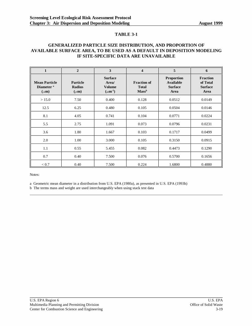
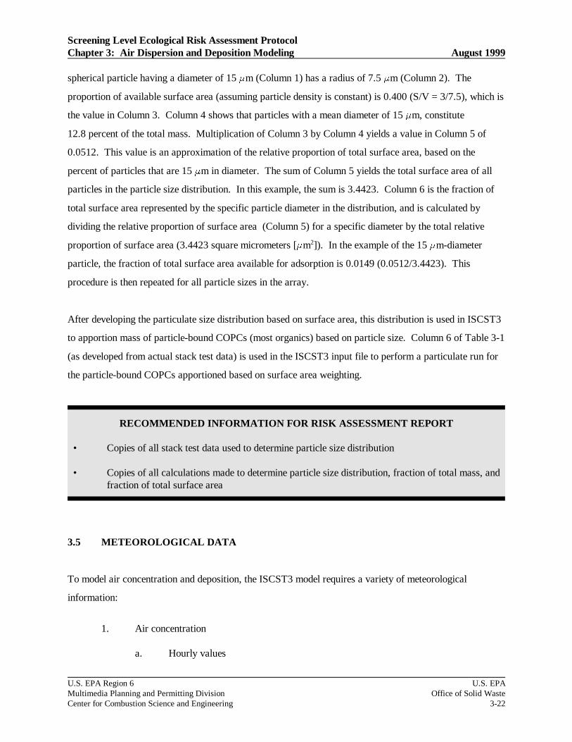
TABLE 3-1
GENERALIZED PARTICLE SIZE DISTRIBUTION, AND PROPORTION OFAVAILABLE SURFACE AREA, TO BE USED AS A DEFAULT IN DEPOSITION MODELING
IF SITE-SPECIFIC DATA ARE UNAVAILABLE
1 2 3 4 5 6
Mean ParticleDiameter a
(Fm)
ParticleRadius(Fm)
SurfaceArea/
Volume(Fm-1)
Fraction ofTotalMassb
ProportionAvailableSurface
Area
Fractionof TotalSurface Area
> 15.0 7.50 0.400 0.128 0.0512 0.0149
12.5 6.25 0.480 0.105 0.0504 0.0146
8.1 4.05 0.741 0.104 0.0771 0.0224
5.5 2.75 1.091 0.073 0.0796 0.0231
3.6 1.80 1.667 0.103 0.1717 0.0499
2.0 1.00 3.000 0.105 0.3150 0.0915
1.1 0.55 5.455 0.082 0.4473 0.1290
0.7 0.40 7.500 0.076 0.5700 0.1656
< 0.7 0.40 7.500 0.224 1.6800 0.4880
Notes:
a Geometric mean diameter in a distribution from U.S. EPA (1980a), as presented in U.S. EPA (1993h)b The terms mass and weight are used interchangeably when using stack test data

Screening Level Ecological Risk Assessment ProtocolChapter 3: Air Dispersion and Deposition Modeling August 1999
U.S. EPA Region 6 U.S. EPAMultimedia Planning and Permitting Division Office of Solid WasteCenter for Combustion Science and Engineering 3-20
From Table 3-1, the mean particle diameter is 5.5 Fm. The mass of particulate from the 5.0 Fm stack test
data is then assigned to the 5.5 Fm mean particle diameter for the purpose of computing the “fraction of
total mass.”
Typically, eight to ten mean particle diameters are available from stack test results. As determined from a
sensitivity analysis conducted by The Air Group-Dallas under contract to U.S. EPA Region 6
(www.epa.gov/region06), a minimum of three particle size categories (> 10 microns, 2-10 microns, and < 2
microns) detected during stack testing are generally the most sensitive to air modeling with ISCST-3 (U.S.
EPA 1997). For facilities with stack test results which indicate mass amounts lower than the detectable
limit (or the filter weight is less after sampling than before), a single mean particle size diameter of 1.0
microns should be used to represent all mass (e.g., particle diameter of 1.0 microns or a particle mass
fraction of 1.0) in the particle and particle-bound model runs. Because rudimentary methods for stack
testing may not detect the very small size or amounts of COPCs in the particle phase, the use of a 1.0
micron particle size will allow these small particles to be included properly as particles in the risk
assessment exposure pathways while dispersing and depositing in the air model similar in behavior to a
vapor.
After calculating the mean particle diameter (Column 1), the fraction of total mass (Column 4) per mean
particle size diameter must be computed from the stack test results. For each mean particle diameter, the
stack test data provides an associated mass of particulate. The fraction of total mass for each mean
particle diameter is calculated by dividing the associated mass of particulate for that diameter by the total
mass of particulate in the sample. In many cases, the fractions of total mass will not sum to 1.0 due to
rounding errors. In these instances, U.S. EPA OSW advocates that the remaining mass fraction be added
into the largest mean particle diameter mass fraction to force the total mass to 1.0.
Direct measurements of particle-size distributions at a proposed new facility may be unavailable, so it will
be necessary to provide assumed particle distributions for use in ISCST3. In such instances, a
representative distribution may be used. The unit on which the representative distribution is based should
be as similar as practicable to the proposed unit. For example, the default distribution provided in
Table 3-1 is not appropriate for a hazardous waste burning boiler with no APCD or a wet scrubber,
because it is based on data from different type of unit. However, the generalized particle size (diameter)
distribution in Table 3-1 may be used as a default for some combustion facilities equipped with either ESPs

Screening Level Ecological Risk Assessment ProtocolChapter 3: Air Dispersion and Deposition Modeling August 1999
U.S. EPA Region 6 U.S. EPAMultimedia Planning and Permitting Division Office of Solid WasteCenter for Combustion Science and Engineering 3-21
or fabric filters, because the distribution is relatively typical of particle size arrays that have been measured
at the outlet to advanced equipment designs (Buonicore and Davis 1992; U.S. EPA 1986a; U.S. EPA
1987a).
After developing the particulate size distribution based on mass, this distribution is used in ISCST3 to
apportion the mass of particle phase COPCs (metals and organics with Fv values less than 0.05) based on
particle size. Column 4 of Table 3-1 (as developed from actual stack test data) is used in the ISCST3 input
file to perform a particulate run with the particle phase COPCs apportioned based on mass weighting.
3.4.3 Particle-Bound Modeling (Surface Area Weighting)
A surface area weighting, instead of mass weighting, of the particles is used in separate particle runs of
ISCST3. Surface area weighting approximates the situation where a semivolatile organic contaminant that
has been volatilized in the high temperature environment of a combustion system and then condensed to the
surface of particles entrained in the combustion gas after it cools in the stack. Thus, the apportionment of
emissions by particle diameter becomes a function of the surface area of the particle that is available for
chemical adsorption (U.S. EPA 1993h).
The first step in apportioning COPC emissions by surface area is to calculate the proportion of available
surface area of the particles. If particle density is held constant (such as 1 g/m3), the proportion of
available surface area of aerodynamic spherical particles is the ratio of surface area (S) to volume (V), as
follows:
• Assume aerodynamic spherical particles.
• Specific surface area of a spherical particle with a radius, r—S = 4 r2
• Volume of a spherical particle with a radius, r—V = 4/3 r3
• Ratio of S to V—S/V = 4 r2/ (4/3 r3) = 3/r
The following uses the particle size distribution in Table 3-1 as an example of apportioning the emission
rate of the particle-bound portion of the COPC based on surface area. This procedure can be followed for
apportioning actual emissions to the actual particle size distribution measured at the stack. In Table 3-1, a
Screening Level Ecological Risk Assessment ProtocolChapter 3: Air Dispersion and Deposition Modeling August 1999
U.S. EPA Region 6 U.S. EPAMultimedia Planning and Permitting Division Office of Solid WasteCenter for Combustion Science and Engineering 3-22
• Copies of all stack test data used to determine particle size distribution
• Copies of all calculations made to determine particle size distribution, fraction of total mass, andfraction of total surface area
RECOMMENDED INFORMATION FOR RISK ASSESSMENT REPORT
spherical particle having a diameter of 15 Fm (Column 1) has a radius of 7.5 Fm (Column 2). The
proportion of available surface area (assuming particle density is constant) is 0.400 (S/V = 3/7.5), which is
the value in Column 3. Column 4 shows that particles with a mean diameter of 15 Fm, constitute
12.8 percent of the total mass. Multiplication of Column 3 by Column 4 yields a value in Column 5 of
0.0512. This value is an approximation of the relative proportion of total surface area, based on the
percent of particles that are 15 Fm in diameter. The sum of Column 5 yields the total surface area of all
particles in the particle size distribution. In this example, the sum is 3.4423. Column 6 is the fraction of
total surface area represented by the specific particle diameter in the distribution, and is calculated by
dividing the relative proportion of surface area (Column 5) for a specific diameter by the total relative
proportion of surface area (3.4423 square micrometers [Fm2]). In the example of the 15 Fm-diameter
particle, the fraction of total surface area available for adsorption is 0.0149 (0.0512/3.4423). This
procedure is then repeated for all particle sizes in the array.
After developing the particulate size distribution based on surface area, this distribution is used in ISCST3
to apportion mass of particle-bound COPCs (most organics) based on particle size. Column 6 of Table 3-1
(as developed from actual stack test data) is used in the ISCST3 input file to perform a particulate run for
the particle-bound COPCs apportioned based on surface area weighting.
3.5 METEOROLOGICAL DATA
To model air concentration and deposition, the ISCST3 model requires a variety of meteorological
information:
1. Air concentration
a. Hourly values

Screening Level Ecological Risk Assessment ProtocolChapter 3: Air Dispersion and Deposition Modeling August 1999
U.S. EPA Region 6 U.S. EPAMultimedia Planning and Permitting Division Office of Solid WasteCenter for Combustion Science and Engineering 3-23
• Identification of all sources of meteorological data
RECOMMENDED INFORMATION FOR RISK ASSESSMENT REPORT
(1) Wind direction (degrees from true north)(2) Wind speed (m/s)(3) Dry bulb (ambient air) temperature (K)(4) Opaque cloud cover (tenths)(5) Cloud ceiling height (m)
b. Daily values
(1) Morning mixing height (m)(2) Afternoon mixing height (m)
2. Deposition
a. Dry particle deposition—hourly values for surface pressure (millibars)
b. Wet particle deposition—hourly values(1) Precipitation amount (inches)(2) Precipitation type (liquid or frozen)
c. Dry vapor deposition (when available)—hourly values for solar radiation(watts/m2)
As shown in Figure 3-1, these data are available from several different sources. For most air modeling,
five years of data from a representative National Weather Service station is recommended. However, in
some instances where the closest NWS data is clearly not representative of site specific meteorlogical
conditions, and there is insufficient time to collect 5 years of onsite data, 1 year of onsite meteorological
data (consistent with GAQM) may be used to complete the risk assessment. The permitting authority
should approve the representative meteorological data prior to performing air modeling.
The following subsections describe how to select the surface and upper air data that will be used in
conjunction with the ISCST3 model. Section 3.7 describes the computer programs used to process the
meteorological data for input to the ISCST3 model.

Screening Level Ecological Risk Assessment ProtocolChapter 3: Air Dispersion and Deposition Modeling August 1999
U.S. EPA Region 6 U.S. EPAMultimedia Planning and Permitting Division Office of Solid WasteCenter for Combustion Science and Engineering 3-24
FIGURE 3-1
SOURCES OF METEOROLOGICAL DATA

Screening Level Ecological Risk Assessment ProtocolChapter 3: Air Dispersion and Deposition Modeling August 1999
U.S. EPA Region 6 U.S. EPAMultimedia Planning and Permitting Division Office of Solid WasteCenter for Combustion Science and Engineering 3-25
3.5.1 Surface Data
Surface data can be obtained from SAMSON in CD-ROM format. SAMSON data are available for 239
airports across the U.S. for the period of 1961 through 1990. The National Climate Data Center (NCDC)
recently released the update to SAMSON through 1995 surface data. However, since the upper air (mixing
height) data available from the U.S. EPA SCRAM web site has not been updated to cover this recent data
period, it is acceptable to select the representative 5 years of meteorological data from the period up
through 1990. SAMSON data contain all of the required input parameters for concentration,
dry and wet particle deposition, and wet vapor deposition. SAMSON also includes the total solar radiation
data required for dry vapor deposition, which may be added to ISCST3 in the future. Alternatively, some
meteorological files necessary for running ISCST3 are also available on the SCRAM BBS for NWS
stations located throughout the country (SCRAM BBS is part of the Office of Air Quality and Planning
and Standards Technology Transfer Network [OAQPS TTN]). The meteorological data, preprocessors,
and user’s guides are also located on the SCRAM web site at “http://www.epa.gov/scram001/index.htm”.
However, these files do not contain surface pressure, types of precipitation (present weather), or
precipitation amount. Although the ISCST3 model is not very sensitive to surface pressure variations, and
a default value may be used, precipitation types and amounts are necessary for air modeling wet deposition.
Precipitation data are available from the National Climatic Data Center (NCDC), and are processed by
PCRAMMET to supplement the SCRAM BBS surface data. NCDC also has surface data in CD-144
format, which contains all of the surface data, including precipitation.
The SAMSON CD-ROM for the eastern, central, or western (Volumes I, II, and III) United States may be
purchased from NCDC in Asheville, North Carolina.

Screening Level Ecological Risk Assessment ProtocolChapter 3: Air Dispersion and Deposition Modeling August 1999
U.S. EPA Region 6 U.S. EPAMultimedia Planning and Permitting Division Office of Solid WasteCenter for Combustion Science and Engineering 3-26
National Climatic Data CenterFederal Building
37 Battery Park AvenueAsheville, NC 28801-2733
Customer Service: (704) 271-4871
File type: File name:
Hourly precipitation amounts NCDC TC-3240
Hourly surface observations with precipitation type NCDC TD-3280
Hourly surface observations with precipitation type NCDC SAMSON CD-ROM (Vol. I, II, and/or III)
Twice daily mixing heights from nearest station NCDC TD-9689(also available on SCRAM web site for 1984 through 1991)
PCRAMMET and MPRM are the U.S. EPA meteorological preprocessor programs for preparing the
surface and upper air data into a meteorlogical file of hourly parameters for input into the ISCST3 model.
Most air modeling analyses will use PCRAMMET to process the National Weather Service data.
However, both preprocessors require the modeler to replace any missing data. Before running
PCRAMMET or MPRM, the air modeler must fill in missing data to complete 1 full year of values. A
procedure recommended by U.S. EPA for filling missing surface and mixing height data is documented on
the SCRAM BBS under the meteorological data section. If long periods of data are missing, and these data
are not addressed by the U.S. EPA procedures on the SCRAM BBS, then a method must be developed for
filling in missing data. One option is to fill the time periods with “surrogate place holder” data in the
correct format with correct sequential times to complete preparation of the meteorological file. Place
holder data are typically considered the last valid hourly data of record. Then, when ISCST3 is running,
the MSGPRO keyword in the COntrol pathway can be used to specify that data are missing. Note that the
DEFAULT keyword must not be used with MSGPRO. Since the missing data keyword is not approved
generally for regulatory air modeling, the appropriate agency must provide approval prior to use. All
processing of meteorological data should be completely documented to include sources of data, decision
criteria for selection, consideration for precipitation amounts, preprocessor options selected, and filled
missing data.
The most recently available 5 years of complete meteorological data contained on SAMSON, or more
recent sources, should be used for the air modeling. It is desirable, but not mandatory, that the 5 years are

Screening Level Ecological Risk Assessment ProtocolChapter 3: Air Dispersion and Deposition Modeling August 1999
U.S. EPA Region 6 U.S. EPAMultimedia Planning and Permitting Division Office of Solid WasteCenter for Combustion Science and Engineering 3-27
• Electronic copy of the ISCST3 input code used to enter meteorological information
• Description of the selection criteria and process used to identify representative years used formeteorological data
• Identification of the 5 years of meteorological selected
• Summary of the procedures used to compensate for any missing data
RECOMMENDED INFORMATION FOR RISK ASSESSMENT REPORT
consecutive. The use of less than five years of meteorological data should be approved by appropriate
authorities. The following subsections describe important characteristics of the surface data.
3.5.1.1 Wind Speed and Wind Direction
Wind speed and direction are two of the most critical parameters in ISCST3. The wind direction promotes
higher concentration and deposition if it persists from one direction for long periods during a year. A
predominantly south wind, such as on the Gulf Coast, will contribute to high concentrations and
depositions north of the facility. Wind speed is inversely proportional to concentration in the ISCST3
algorithms. The higher the wind speed, the lower will be the concentration. If wind speed doubles, the
concentration and deposition will be reduced by one-half. ISCST3 needs wind speed and wind direction at
the stack top. Most air modeling is performed using government sources of surface data. Wind data are
typically measured at 10 meters height at NWS stations. However, since some stations have wind speed
recorded at a different height, the anemometer height must always be verified so that the correct value can
be input into the PCRAMMET meteorological data preprocessing program. ISCST3 assumes that wind
direction at stack height is the same as measured at the NWS station height. ISCST3 uses a wind speed
profile to calculate wind speed at stack top. This calculation exponentially increases the measured wind
speed from the measured height to a calculated wind speed at stack height (U.S. EPA 1995d).
3.5.1.2 Dry Bulb Temperature
Dry bulb temperature, or ambient air temperature, is the same temperature reported on the television and
radio stations across the country each day. It is measured at 2 meters above ground level. Air temperature

Screening Level Ecological Risk Assessment ProtocolChapter 3: Air Dispersion and Deposition Modeling August 1999
U.S. EPA Region 6 U.S. EPAMultimedia Planning and Permitting Division Office of Solid WasteCenter for Combustion Science and Engineering 3-28
is used in ISCST3 in the buoyant plume rise equations developed by Briggs (U.S. EPA 1995c). The model
results are not very sensitive to air temperature, except at extremes. However, buoyant plume rise is very
sensitive to the stack gas temperature. Buoyant plume rise is mainly a result of the difference between
stack gas temperature and ambient air temperature. Conceptually, it is similar to a hot air balloon. The
higher the stack gas temperature, the higher will be the plume rise. High plume heights result in low
concentrations and depositions as the COPCs travel further and are diluted in a larger volume of ambient
air before reaching the surface. The temperature is measured in K, so a stack gas temperature of 450EF is
equal to 505 K. Ambient temperature of 90EF is equal to 305 K, and 32EF is 273 K. A large variation in
ambient temperature will affect buoyant plume rise, but not as much as variations in stack gas temperature.
3.5.1.3 Opaque Cloud Cover
PCRAMMET uses opaque cloud cover to calculate the stability of the atmosphere. Stability determines
the dispersion, or dilution, rate of the COPCs. Rapid dilution occurs in unstable air because of surface
heating that overturns the air. With clear skies during the day, the sun heats the Earth’s surface, thereby
causing unstable air and dilution of the stack gas emission stream. Stable air results in very little mixing,
or dilution, of the emitted COPCs. A cool surface occurs at night because of radiative loss of heat on clear
nights. With a cloud cover, surface heating during the day and heat loss at night are reduced, resulting in
moderate mixing rates, or neutral stability. Opaque cloud cover is a measure of the transparency of the
clouds. For example, a completely overcast sky with 10/10ths cloud cover may have only 1/10th opaque
cloud cover if the clouds are high, translucent clouds that do not prevent sunlight from reaching the Earth’s
surface. The opaque cloud cover is observed at NWS stations each hour.
3.5.1.4 Cloud Ceiling Height
Cloud height is required in PCRAMMET to calculate stability. Specifically, the height of the cloud cover
affects the heat balance at the Earth’s surface. Cloud ceiling height is measured or observed at all NWS
stations provided on the SAMSON CD-Roms and the U.S. EPA SCRAM web site.

Screening Level Ecological Risk Assessment ProtocolChapter 3: Air Dispersion and Deposition Modeling August 1999
U.S. EPA Region 6 U.S. EPAMultimedia Planning and Permitting Division Office of Solid WasteCenter for Combustion Science and Engineering 3-29
3.5.1.5 Surface Pressure
Surface pressure is required by ISCST3 for calculating dry particle deposition. However, ISCST3 is not
very sensitive to surface pressure. SAMSON and NCDC CD-144 data include surface pressure. SCRAM
BBS surface data do not include surface pressure. U.S. EPA believes that, if SCRAM BBS surface data
are used, a default value of 1,000 millibars can be assumed, with little impact on modeled results.
3.5.1.6 Precipitation Amount and Type
The importance of precipitation to ISCST3 results was discussed in the selection of the meteorological data
period (see Section 3.5.1). Precipitation is measured at 3 feet (1 meter) above ground level. Precipitation
amount and type are required to be processed by PCRAMMET or MPRM into the ISCST3 meteorological
file to calculate wet deposition of vapor and particles. The amount of precipitation, or precipitation rate,
will directly influence the amount of wet deposition at a specific location. Particles and vapor are both
captured by falling precipitation, known as precipitation scavenging. Scavenging coefficients are required
as inputs to ISCST3 for vapors with a rate specified for liquid and frozen precipitation. The precipitation
type in a weather report in SAMSON or CD-144 data file will identify to ISCST3 which event is occurring
for appropriate use of the scavenging coefficients entered (see Section 3.7.2.6). SCRAM BBS surface data
do not include precipitation data. Supplemental precipitation files from NCDC may be read into
PCRAMMET for integration into the ISCST3 meteorological file.
3.5.1.7 Solar Radiation (Future Use for Dry Vapor Deposition)
The current version of ISCST3 does not use solar radiation. Several U.S. EPA models, including the Acid
Deposition and Oxidant Model (ADOM), incorporate algorithms for dry vapor deposition. At such time as
U.S. EPA approves the draft version of ISCST3 which includes dry gas deposition, the hourly total solar
radiation will be required. Solar radiation affects the respiratory activity of leaf surfaces, which affects the
rate of vapor deposition. With a leaf area index identified in the ISCST3 input file in the future, the model
will be able to calculate dry vapor deposition.

Screening Level Ecological Risk Assessment ProtocolChapter 3: Air Dispersion and Deposition Modeling August 1999
U.S. EPA Region 6 U.S. EPAMultimedia Planning and Permitting Division Office of Solid WasteCenter for Combustion Science and Engineering 3-30
3.5.2 Upper Air Data
Upper air data, also referred to as mixing height data, are required to run the ISCST3 model. ISCST3
requires estimates of morning and afternoon (twice daily) mixing heights. PCRAMMET and MPRM use
these estimates to calculate an hourly mixing height by using interpolation methods (U.S. EPA 1996e).
The mixing height files are typically available for the years 1984 through 1991 on the U.S. EPA SCRAM
web site. U.S. EPA OSW recommends that only years with complete mixing height data be used as input
for air modeling. In some instances, data may need to be obtained from more than one station to complete
five years of data. The selection of representative data should be discussed with appropriate authorities
prior to performing air modeling.
Mixing height data for years prior to 1983, in addition to current mixing height data, may be purchased
from NCDC as described in Section 3.5.1. The years selected for upper air data must match the years
selected for surface data. If matching years of mixing height data are not available from a single upper air
station, another upper air station should be used for completing the five years.
3.6 METEOROLOGICAL PREPROCESSORS AND INTERFACE PROGRAMS
After the appropriate surface and upper air data is selected following the procedures outlined in
Section 3.5, additional data manipulation is necessary before the data is used with the ISCST3 model. The
following subsections describe the meteorological preprocessors and interface programs used for these
manipulation tasks. To eliminate any need to repeat air modeling activities, U.S. EPA OSW recommends
that the selection of representative mixing height and surface data be approved by the appropriate
regulatory agency before preprocessing or air modeling is conducted. Permitting authority approval also is
recommended in the selection of site-specific parameter values required as input to the meteorological data
preprocessors.
3.6.1 PCRAMMET
U.S. EPA OSW recommends preparing a meteorological file for ISCST3 that can be used to calculate any
concentration or deposition. By preparing a file that PCRAMMET terms a “WET DEPOSITION” file, all
required parameters will be available to ISCST3 for any subsequent concentration or deposition modeling.

Screening Level Ecological Risk Assessment ProtocolChapter 3: Air Dispersion and Deposition Modeling August 1999
U.S. EPA Region 6 U.S. EPAMultimedia Planning and Permitting Division Office of Solid WasteCenter for Combustion Science and Engineering 3-31
For example, if only the concentration option is selected in ISCST3 for a specific run, ISCST3 will ignore
the precipitation values in the meteorological file. For subsequent air deposition modeling, ISCST3 will
access the precipitation data from the same preprocessed meteorological file.
PCRAMMET may use SAMSON, SCRAM web site, and NCDC CD-144 surface data files. U.S. EPA
OSW recommends using the SAMSON option in PCRAMMET to process the SAMSON surface data and
U.S. EPA SCRAM web site mixing height data. The PCRAMMET User’s Guide in the table “Wet
Deposition, SAMSON Data” (U.S. EPA 1995b) identifies the PCRAMMET input requirements for
creating an ASCII meteorological file for running ISCST3 to calculate air concentration, and wet and dry
deposition. The meteorological file created for ISCST3 will contain all of the parameters needed for air
modeling of concentration and deposition.
PCRAMMET requires the following input parameters representative of the measurement site:
• Monin-Obukhov length
• Anemometer height
• Surface roughness height (at measurement site)
• Surface roughness height (at application site)
• Noon-time albedo
• Bowen ratio
• Anthropogenic heat flux
• Fraction of net radiation absorbed at surface
The PCRAMMET User’s Guide contains detailed information for preparing the required meteorological
input file for the ISCST3 model (U.S. EPA 1995b). The parameters listed are briefly described in the
following subsections. These data are not included in the surface or mixing height data files obtained from
the U.S. EPA or NCDC. Representative values specific to the site to be modeled should be carefully
selected using the tables in the PCRAMMET User’s Guide or reference literature. The selected values
should be approved prior to processing the meteorological data.

Screening Level Ecological Risk Assessment ProtocolChapter 3: Air Dispersion and Deposition Modeling August 1999
U.S. EPA Region 6 U.S. EPAMultimedia Planning and Permitting Division Office of Solid WasteCenter for Combustion Science and Engineering 3-32
3.6.1.1 Monin-Obukhov Length
The Monin-Obukhov length (L) is a measure of atmospheric stability. It is negative during the day, when
surface heating causes unstable air. It is positive at night, when the surface is cooled with a stable
atmosphere. In urban areas during stable conditions, the estimated value of L may not adequately reflect
the less stable atmosphere associated with the mechanical mixing generated by buildings or structures.
However, PCRAMMET requires an input for minimum urban Monin-Obukhov length, even if the area to
be analyzed by ISCST3 is rural. A nonzero value for L must be entered to prevent PCRAMMET from
generating an error message. A value of 2.0 meter for L should be used when the land use surrounding the
site is rural (see Section 3.2.2.1). For urban areas, Hanna and Chang (1991) suggest that a minimum value
of L be set for stable hours to simulate building-induced instability. The following are general examples of
L values for various land use classifications:
Land Use Classification Minimum L
Agricultural (open) 2 meters
Residential 25 meters
Compact residential/industrial 50 meters
Commercial (19 to 40-story buildings) 100 meters
Commercial (>40-story buildings) 150 meters
PCRAMMET will use the minimum L value for calculating urban stability parameters. These urban
values will be ignored by ISCST3 during the air modeling analyses for rural sites.
3.6.1.2 Anemometer Height
The height of the wind speed measurements is required by ISCST3 to calculate wind speed at stack top.
The wind sensor (anemometer) height is identified in the station history section of the Local Climatological
Data Summary available from NCDC for every National Weather Service station. Since 1980, most
National Weather Service stations measure wind speed at the height of 10 meters. However, some stations
operate at other heights or have valid representative data during years of operation at more than one height.
The modeler must verify the correct measurement height for each year of data prior to processing with

Screening Level Ecological Risk Assessment ProtocolChapter 3: Air Dispersion and Deposition Modeling August 1999
U.S. EPA Region 6 U.S. EPAMultimedia Planning and Permitting Division Office of Solid WasteCenter for Combustion Science and Engineering 3-33
PCRAMMET and running the ISCST3 model. ISCST3 modeled results are very sensitive to small
variations in wind speed.
3.6.1.3 Surface Roughness Height at Measurement Site
Surface roughness height is a measure of the height of obstacles to wind flow. It is important in ISCST3
because it determines how close a particle must be above the ground before it is “captured” for deposition
on the ground. Dramatic differences in ISCST3 calculations may result from slight variations in surface
roughness. For surface meteorological data from a National Weather Station, a value of 0.10 meters for
the “measurement site” typically may be used without prior approval. Surface roughness is proportional,
but not equal, to the physical height of the obstacles. The table in Section 3.2.2.2 lists the roughness
heights that can be used as input values. These values are based on the general land use in the vicinity of
the measurement site. These values should be considered in discussions with the appropriate agency
modeler prior to air modeling.
3.6.1.4 Surface Roughness Height at Application Site
Determination of surface roughness height is also required at the facility (application site) for performing
PCRAMMET processing to prepare an ISCST3 meteorological file. ISCST3 model results are very
sensitive to the value used in PCRAMMET for this parameter. The table in Section 3.2.2.2 is applicable to
the application site. A site-specific computation of a single surface roughness value representative of the
site is required using the method described in Section 3.2.2.2. The computed value of surface roughness
height for the application site, along with maps or photographs illustrating land use, must be approved by
the appropriate agency prior to use.
3.6.1.5 Noon-Time Albedo
“Noon-time albedo” is the fraction of the incoming solar radiation that is reflected from the ground when
the sun is directly overhead. Albedo is used in calculating the hourly net heat balance at the surface for
calculating hourly values of Monin-Obukhov length. PCRAMMET automatically adjusts for the variation
in albedo with solar elevation angle. Experience suggests that ISCST3 modeling results are not sensitive to
the value selected for this parameter. Typical albedo values are presented in Table 3-2. As shown in Table

Screening Level Ecological Risk Assessment ProtocolChapter 3: Air Dispersion and Deposition Modeling August 1999
U.S. EPA Region 6 U.S. EPAMultimedia Planning and Permitting Division Office of Solid WasteCenter for Combustion Science and Engineering 3-34
3-2, albedo values vary from 0.10 to 0.20 on water surfaces from summer to winter. The most variability
is for cultivated farmland, which varies from 0.14 during spring when land is tilled to expose dark earth, to
0.60 in winter when areas are snow-covered.
Based on the information in Table 3-2, albedos are estimated to vary in rural areas from 0.14 to 0.20 for
cultivated land, and from 0.18 to 0.20 for grassland. For urban areas, the variation without snow is from
0.14 to 0.18. For practical purposes, the selection of a single value for noon-time albedo to process a
complete year of meteorological data is desirable. For example, the single value of 0.18 may be
appropriate to process all meteorological data for an urban site. For rural sites, a single albedo value of
0.18 representative of grassland and cultivated land may be appropriate for areas without significant snow
cover during winter months. For desert shrubland, a single value of 0.28 may be appropriate. A single
value of 0.12 could be representative of forested areas. The permitting authority should review proposed
values used in the processing of the meteorological data.

Screening Level Ecological Risk Assessment ProtocolChapter 3: Air Dispersion and Deposition Modeling August 1999
U.S. EPA Region 6 U.S. EPAMultimedia Planning and Permitting Division Office of Solid WasteCenter for Combustion Science and Engineering 3-35
TABLE 3-2
ALBEDO OF NATURAL GROUND COVERS FOR LAND USE TYPES AND SEASONS
Land Use TypeSeasona
Spring Summer Autumn Winter
Water surface 0.12 0.10 0.14 0.20
Deciduous forest 0.12 0.12 0.12 0.50
Coniferous forest 0.12 0.12 0.12 0.35
Swamp 0.12 0.14 0.16 0.30
Cultivated land 0.14 0.20 0.18 0.60
Grassland 0.18 0.18 0.20 0.60
Urban 0.14 0.16 0.18 0.35
Desert shrubland 0.30 0.28 0.28 0.45
Notes:
Source—Iqbal (1983)
a The various seasons are defined by Iqbal (1983) as follows:
Spring: Periods when vegetation is emerging or partially green; this is a transitional situation that appliesfor 1 to 2 months after the last killing frost in spring.
Summer: Periods when vegetation is lush and healthy; this is typical of mid-summer, but also of otherseasons in which frost is less common.
Autumn: Periods when freezing conditions are common, deciduous trees are leafless, crops are not yetplanted or are already harvested (bare soil exposed), grass surfaces are brown, and no snow ispresent.
Winter: Periods when surfaces are covered by snow and temperatures are below freezing. Winter albedodepends on whether a snow cover is present continuously, intermittently, or seldom. Albedoranges from about 0.30 for bare snow cover to about 0.65 for continuous cover.

Screening Level Ecological Risk Assessment ProtocolChapter 3: Air Dispersion and Deposition Modeling August 1999
U.S. EPA Region 6 U.S. EPAMultimedia Planning and Permitting Division Office of Solid WasteCenter for Combustion Science and Engineering 3-36
3.6.1.6 Bowen Ratio
The Bowen ratio is a measure of the amount of moisture at the surface. The presence of moisture affects
the heat balance resulting from evaporative cooling, which, in turn, affects the hourly Monin-Obukhov
length calculated by PCRAMMET. Surface moisture is highly variable. Daytime Bowen ratios are
presented in Table 3-3.
Bowen ratio values vary throughout the country. For example, in urban areas where annual rainfall is less
than 20 inches, a single Bowen ratio value of 4.0 may be representative. For rural areas, a Bowen ratio
value of 2.0 may be appropriate for grassland and cultivated land. For areas where annual rainfall is
greater than 20 inches, U.S. EPA OSW recommends a single Bowen ratio value of 2.0 for urban areas;
and 0.7 for rural forests, grasslands, and cultivated lands. The applicable permiting authority should
review proposed values used in the processing of the meteorological data.
3.6.1.7 Anthropogenic Heat Flux
Anthropogenic heat is the surface heating caused by human activity, including automobiles and heating
systems. It is used to calculate hourly L values (Monin-Obukhov lengths). Table 3-4 presents
anthropogenic heat flux (Qf) values that have been calculated for several urban areas around the world. In
rural areas, U.S. EPA OSW recommends that a value of 0.0 Watts/m2 be used for the Qf. A value of 20.0
Watts/m2 is appropriate for large urban areas based on the annual value from Table 3-4 for Los Angeles.
3.6.1.8 Fraction of Net Radiation Absorbed at the Ground
Also used for calculating hourly values of Monin-Obukhov length, fraction of net radiation absorbed at the
ground is the last component of radiative heat balance. Based on the net radiation (Q*) values presented in
Table 3-4, and recommendations presented in the PCRAMMET User’s Manual based on Oke (1982),
U.S. EPA OSW recommends values of 0.15 for rural areas and 0.27 for urban areas (U.S. EPA 1995b).

Screening Level Ecological Risk Assessment ProtocolChapter 3: Air Dispersion and Deposition Modeling August 1999
U.S. EPA Region 6 U.S. EPAMultimedia Planning and Permitting Division Office of Solid WasteCenter for Combustion Science and Engineering 3-37
TABLE 3-3
DAYTIME BOWEN RATIOS BY LAND USE, SEASON,AND PRECIPITATION CONDITIONS
Land UseSeasona
Spring Summer Autumn Winter
Dry Conditions
Water (fresh and salt) 0.1 0.1 0.1 2.0
Deciduous forest 1.5 0.6 2.0 2.0
Coniferous forest 1.5 0.6 1.5 2.0
Swamp 0.2 0.2 0.2 2.0
Cultivated land 1.0 1.5 2.0 2.0
Grassland 1.0 2.0 2.0 2.0
Urban 2.0 4.0 4.0 2.0
Desert shrubland 5.0 6.0 10.0 2.0
Average Conditions
Water (fresh and salt) 0.1 0.1 0.1 1.5
Deciduous forest 0.7 0.3 1.0 1.5
Coniferous forest 0.7 0.3 0.8 1.5
Swamp 0.1 0.1 0.1 1.5
Cultivated land 0.3 0.5 0.7 1.5
Grassland 0.4 0.8 1.0 1.5
Urban 1.0 2.0 2.0 1.5
Desert shrubland 3.0 4.0 6.0 6.0

Screening Level Ecological Risk Assessment ProtocolChapter 3: Air Dispersion and Deposition Modeling August 1999
U.S. EPA Region 6 U.S. EPAMultimedia Planning and Permitting Division Office of Solid WasteCenter for Combustion Science and Engineering 3-38
TABLE 3-3
DAYTIME BOWEN RATIO BY LAND USE, SEASON,AND PRECIPITATION CONDITIONS
(Continued)
Land UseSeasona
Spring Summer Autumn Winter
Wet Conditions
Water (fresh and salt) 0.1 0.1 0.1 0.3
Deciduous forest 0.3 0.2 0.4 0.5
Coniferous forest 0.3 0.2 0.3 0.3
Swamp 0.1 0.1 0.1 0.5
Cultivated land 0.2 0.3 0.4 0.5
Grassland 0.3 0.4 0.5 0.5
Urban 0.5 1.0 1.0 0.5
Desert shrubland 1.0 5.0 2.0 2.0
Note:
Source—Paine (1987)
a The various seasons are defined by Iqbal (1983) as follows:
Spring: Periods when vegetation is emerging or partially green; this is a transitional situationthat applies for 1 to 2 months after the last killing frost in spring.
Summer: Periods when vegetation is lush and healthy; this is typical of mid-summer, but also ofother seasons in which frost is less common.
Autumn: Periods when freezing conditions are common, deciduous trees are leafless, crops arenot yet planted or are already harvested (bare soil exposed), grass surfaces are brown,and no snow is present
Winter: Periods when surfaces are covered by snow and temperatures are below freezing.

Screening Level Ecological Risk Assessment ProtocolChapter 3: Air Dispersion and Deposition Modeling August 1999
U.S. EPA Region 6 U.S. EPAMultimedia Planning and Permitting Division Office of Solid WasteCenter for Combustion Science and Engineering 3-39
TABLE 3-4
ANTHROPOGENIC HEAT FLUX (Qf) AND NET RADIATION (Q*)FOR SEVERAL URBAN AREAS
Urban Area(Latitude)
Population(Millions)
PopulationDensity
(Persons/km2)
Per CapitaEnergy Use
(MJ x 103/year)
Qf (Watts/m2)(Season)
Q*
(Watts/m2)
Manhattan(40E North)
1.7 28,810 128 117 (Annual)40 (Summer)198 (Winter)
93 (Annual)
Montreal(45E North)
1.1 14,102 221 99 (Annual)57 (Summer)153 (Winter)
52 (Annual)92 (Summer)13 (Winter)
Budapest(47E North)
1.3 11,500 118 43 (Annual)32 (Summer)51 (Winter)
46 (Annual)100 (Summer)-8 (Winter)
Sheffield(53E North)
0.5 10,420 58 19 (Annual) 56 (Annual)
West Berlin(52E North)
2.3 9,830 67 21 (Annual) 57 (Annual)
Vancouver(49E North)
0.6 5,360 112 19 (Annual)15 (Summer)23 (Winter)
57 (Annual)107 (Summer)6 (Winter)
Hong Kong (22E North)
3.9 3,730 34 4 (Annual) 110 (Annual)
Singapore(1E North)
2.1 3,700 25 3 (Annual) 110 (Annual)
Los Angeles (34E North)
7.0 2,000 331 21 (Annual) 108 (Annual)
Fairbanks(64E North)
0.03 810 740 19 (Annual) 18 (Annual)
Note:
Source—Oke (1978)

Screening Level Ecological Risk Assessment ProtocolChapter 3: Air Dispersion and Deposition Modeling August 1999
U.S. EPA Region 6 U.S. EPAMultimedia Planning and Permitting Division Office of Solid WasteCenter for Combustion Science and Engineering 3-40
3.6.2 MPRM
For on-site data, a new version of MPRM is used to mesh on-site data with NWS data in the preparation of
the meteorological input file. MPRM performs the same meteorological file preparation as PCRAMMET,
except the source of the surface data in MPRM consists of on-site measurements (U.S. EPA 1996e).
MPRM includes extensive QA/QC for values that are out of range. MPRM also checks for missing data
and summarizes values that require editing to fill missing data. After a complete surface file passes the
quality checks, it is processed with NCDC mixing height data. NCDC data are purchased to correspond to
the collection period of the on-site surface data. Mixing height data available on SCRAM’s web site ends
in 1991. A delay of about 3 months can occur for obtaining mixing height data from NCDC to process
with recent on-site surface data.
Inputs to MPRM for preparing an ISCST3 meteorological file for concentration and deposition are the
same as for PCRAMMET. Section 3.6.1 provides methods for determining values for these parameters.
Draft versions of ISCST3 and MPRM are available for review which implement dry vapor deposition.
These versions are GDISCDFT (dated 96248) and GDMPRDFT (dated 96248), respectively. They may
be found on the U.S. EPA SCRAM web site under “Topics for Review”. These draft models are not the
current regulatory versions and should not be used without approval from the appropriate permitting
authority.
3.7 ISCST3 MODEL INPUT FILES
A thorough instruction of how to prepare the input files for ISCST3 is presented in the ISC3 User’s Guide,
Volume I (U.S. EPA 1995c), which is available for downloading from the SCRAM BBS. The example
ISCST3 input file is provided in Figure 3-2 from the air dispersion modeling chapter (Chapter 3) of the
U.S. EPA HHRAP (U.S. EPA 1998). This example illustrates a single year run (1984), for particle phase
COPC emissions from a single stack, to compute acute (1-hour average) and chronic (annual average) and
provide single year results in one hour and annual average plot files for post-processing. For ecological
risk assessments, only the annual average air parameters are required, not the 1-hour values. However, by
modeling both the 1-hour and annual averages in a single set of runs, the ISCST3 air dispersion model will
Screening Level Ecological Risk Assessment ProtocolChapter 3: Air Dispersion and Deposition Modeling August 1999
U.S. EPA Region 6 U.S. EPAMultimedia Planning and Permitting Division Office of Solid WasteCenter for Combustion Science and Engineering 3-41
provide the necessary air parameters for use in both the human health and ecological risk assessments. The
specification of a terrain grid file in the TG pathway is optional. Each air modeling analysis has unique
issues and concerns that should be addressed in the risk assessment report. U.S. EPA OSW recommends
that the air modeling methodology be consistent in data collection, model set-up, and model output. This
consistency will assist both the modeler and U.S. EPA in communicating and interpreting model results.
The risk assessment report should document each section of the ISCST3 input file to identify consistent
methods.
Three sets of ISCST3 runs are required for each COPC emission source. As discussed in Section 3.4,
separate ISCST3 runs are required to model vapor phase COPCs, particle phase COPCs, and
particle-bound phase COPCs for each source (stack or fugitive) of COPCs. The ISCST3 “Control
Secondary Keywords” used for these three runs are:
Vapor Phase: CONC WDEP
Particle Phase: CONC DDEP WDEP DEPOS
Particle-Bound Phase: CONC DDEP WDEP DEPOS
For ISCST3 modeling to provide air parameters for ecological risk assessments, only the total deposition
(DEPOS) of the particle and particle-bound phases are required. The control secondary keywords for
concentration in the air (CONC) and the components of deposition to the ground, dry deposition (DDEP)
and wet deposition (WDEP), are not required to be output separately by ISCST3. However, by specifying
these control secondary keywords as illustrated, the ISCST3 model will compute the needed air parameters
for both human health and ecological risk assessments. ISCST3 requires site-specific inputs for source
parameters, receptor locations, meteorological data, and terrain features. The model is prepared for

Screening Level Ecological Risk Assessment ProtocolChapter 3: Air Dispersion and Deposition Modeling August 1999
U.S. EPA Region 6 U.S. EPAMultimedia Planning and Permitting Division Office of Solid WasteCenter for Combustion Science and Engineering 3-42
• Electronic and hard copies of ISCST3 input file for all air modeling runs
RECOMMENDED INFORMATION FOR RISK ASSESSMENT REPORT
execution by creating an input file. The input file is structured in five (or six if a terrain grid file is used)
sections, or pathways, designated by two-letter abbreviations:
ISCST3 INPUT FILE SECTIONS
Section Abbreviation
Control CO
Source SO
Receptor RE
Meteorology ME
Terrain Grid (Optional) TG
Output OU
The following subsections describe how to specify the parameters for each pathway in the ISCST3 input
file.
3.7.1 COntrol Pathway
Model options (MODELOPT) are specified in the COntrol pathway to direct ISCST3 in the types of
computations to perform. U.S. EPA OSW recommends that air modeling specify the DFAULT parameter
to use the following regulatory default options:
• Use stack-tip downwash (except for Schulman-Scire downwash).
• Use buoyancy-induced dispersion (except for Schulman-Scire downwash).
• Do not use final plume rise (except for building downwash).
• Use the calms processing routines.

Screening Level Ecological Risk Assessment ProtocolChapter 3: Air Dispersion and Deposition Modeling August 1999
U.S. EPA Region 6 U.S. EPAMultimedia Planning and Permitting Division Office of Solid WasteCenter for Combustion Science and Engineering 3-43
• Use upper-bound concentration estimates for sources influenced by building downwashfrom super-squat buildings.
• Use default wind speed profile exponents.
• Use default vertical potential temperature gradients.
The CONC parameter specifies calculation of air concentrations for vapor and particles. The DDEP and
WDEP parameters specify dry and wet deposition. The DEPOS specifies computation of total (wet and dry)
deposition flux. Since ISCST3 currently does not include an algorithm for the dry deposition of vapor
phase COPCs, only wet deposition is specified for vapor phase runs. Note that dry deposition of vapor
phase is addressed in the pathway equations during the risk assessment using the concentration of the vapor
phase and a deposition velocity. DRYDPLT and WETDPLT are used for plume depletion resulting from dry
and wet removal. U.S. EPA OSW recommends the following command lines for each of the three runs
(these are for rural areas; substitute URBAN for urban areas):
Vapor: CO MODELOPT DFAULT CONC WDEP WETDPLT RURAL
Particle Phase: CO MODELOPT DFAULT CONC DDEP WDEP DEPOS DRYDPLT WETDPLTRURAL
Particle-Bound: CO MODELOPT DFAULT CONC DDEP WDEP DEPOS DRYDPLT WETDPLTRURAL
Note that only the total deposition (DEPOS) air parameter values are required for the ecological risk assessment
pathways. The modeler may elect not to include CONC, DDEP and WDEP as separate output components
from ISCST3 if the air modeling results will not be used for a human health risk assessment. However, the
control secondary keywords must always be specified for plume depletion through the dry deposition
(DRYDPLT) and wet deposition (WETDPLT) processes.

Screening Level Ecological Risk Assessment ProtocolChapter 3: Air Dispersion and Deposition Modeling August 1999
U.S. EPA Region 6 U.S. EPAMultimedia Planning and Permitting Division Office of Solid WasteCenter for Combustion Science and Engineering 3-44
FIGURE 3-2
EXAMPLE INPUT FILE FOR “PARTICLE PHASE”
CO STARTINGCO TITLEONE Example input file, particle phase runCO TITLETWO 1984 met data, Baton Rouge Surface, Boothville Upper AirCO MODELOPT DFAULT CONC DDEP WDEP DEPOS DRYDPLT WETDPLT RURALCO AVERTIME 1 ANNUALCO POLLUTID UNITYCO TERRHGTS ELEVCO RUNORNOT RUNCO SAVEFILE 84SAVE1 5 84SAVE2** Restart incomplete runs with INITFILE, changing ’**’ to ’CO’** INITFILE 84SAVE1CO FINISHED
SO STARTINGSO LOCATION STACK1 POINT 637524. 567789. 347.SO SRCPARAM STACK1 1.0 23.0 447.0 14.7 1.9SO BUILDHGT STACK1 18.29 18.29 18.29 18.29 18.29 18.29 18.29 18.29SO BUILDHGT STACK1 18.29 18.29 18.29 18.29 18.29 18.29 18.29 18.29SO BUILDHGT STACK1 18.29 18.29 18.29 18.29 18.29 18.29 18.29 18.29SO BUILDHGT STACK1 18.29 18.29 18.29 18.29 18.29 18.29 18.29 18.29SO BUILDHGT STACK1 18.29 18.29 18.29 18.29SO BUILDWID STACK1 14.02 15.51 16.53 17.05 17.05 16.53 15.51 14.03SO BUILDWID STACK1 12.10 14.02 15.51 16.53 17.05 17.05 16.53 15.51SO BUILDWID STACK1 14.02 12.10 14.02 15.51 16.53 17.05 17.05 16.53SO BUILDWID STACK1 15.51 14.02 12.10 14.02 15.51 16.53 17.05 17.05SO BUILDWID STACK1 16.53 15.51 14.02 12.10SO PARTDIAM STACK1 0.35 0.70 1.10 2.00 3.60 5.50 8.10 12.5 15.0SO MASSFRAX STACK1 0.22 0.08 0.08 0.11 0.10 0.07 0.10 0.11 0.13SO PARTDENS STACK1 1.0 1.0 1.0 1.0 1.0 1.0 1.0 1.0 1.0 SO PARTSLIQ STACK1 7E-5 5E-5 6E-5 1.3E-4 2.6E-4 3.9E-4 5.2E-4 6.7E-4 6.7E-4 SO PARTSICE STACK1 2E-5 2E-5 2E-5 4E-5 9E-5 1.3E-4 1.7E-4 2.2E-4 2.2E-4 SO SRCGROUP ALLSO FINISHED
RE STARTINGRE ELEVUNIT METERSRE DISCCART 630000. 565000. 352.RE DISCCART 630500. 565000. 365.RE DISCCART 631000. 565000. 402. ... (ARRAY OF DISCRETE RECEPTORS) ...RE DISCCART 635000. 570000. 387.RE FINISHED
ME STARTINGME INPUTFIL 84BTR.WETME ANEMHGHT 10.0ME SURFDATA 13970 1984 BATON_ROUGEME UAIRDATA 12884 1984 BOOTHVILLEME FINISHED
TG STARTINGTG INPUTFIL TERRAIN.TERTG LOCATION 0.0 0.0TG ELEVUNIT METERSTG FINISHED
OU STARTINGOU RECTABLE ALLAVE FIRSTOU PLOTFILE 1 ALL FIRST BTR841.PLTOU PLOTFILE ANNUAL ALL BTR84A.PLTOU FINISHED

Screening Level Ecological Risk Assessment ProtocolChapter 3: Air Dispersion and Deposition Modeling August 1999
U.S. EPA Region 6 U.S. EPAMultimedia Planning and Permitting Division Office of Solid WasteCenter for Combustion Science and Engineering 3-45
For each of the three runs for each emission source, 5 years of off-site (e.g., National Weather Service
from SAMSON) meteorological data are completed. For sites with meteorological data collected on-site,
the appropriate permitting authority should be notified for the data period required for a risk assessment.
The averaging times (AVERTIME) should be specified as ‘ANNUAL’ to compute long-term (annual
average) ecological risk. Optionally, the ‘1' may be specified for convenience in modeling for the
maximum 1-hour averages used in computing acute human health risks. Each phase run may be repeated
five times (one for each year, or a total of 15 ISCST3 runs) to complete a set of 15 runs for the full five
years of meteorological data.
Alternatively, the modeler may combine the 5 years of meteorological data into a single meteorological data
file and complete only 3 runs for each emission source (one run for each phase). Section 3.5.1.1 of the
ISC3 User’s Guide (U.S. EPA 1995c), includes a complete discussion of combining multiple years of
meteorological data into a single file prior to running ISCST3. The modeler should select the ‘ANNUAL’
averaging time for all risk assessment runs, regardless of the number of years in the meteorological data
file. The incorrect selection of ‘PERIOD’ will not compute the correct deposition rates required by the risk
assessment equations (refer to Section 3.2.3 of the ISC3 User Guide, Volume I). No additional ISCST3
model execution time is required to obtain 1-year or 5-year air modeling values.
In addition, ISCST3 allows the specification of COPC half-life and decay coefficients. Unless approved by
the permitting authority with documentation of COPC-specific data, these keywords should not be used
when conducting air modeling to support risk assessments. The TERRHGTS keyword with the ELEV
parameter typically should be used to model terrain elevations at receptor grid nodes. The FLAGPOLE
keyword specifies receptor grid nodes above local ground level and is not typically used for most air
modeling to perform impacts at ground level.
U.S. EPA OSW also recommends that SAVEFIL be used to restart ISCST3 in the event of a computer or
power failure during long runs. SAVEFIL is best used by specifying two save files, each with a different
name. The save interval should be no longer than 5 days for large runs. If two save files are used, and a

Screening Level Ecological Risk Assessment ProtocolChapter 3: Air Dispersion and Deposition Modeling August 1999
U.S. EPA Region 6 U.S. EPAMultimedia Planning and Permitting Division Office of Solid WasteCenter for Combustion Science and Engineering 3-46
failure occurs during writing to the savefile, no more than 10 days will be lost. The INITFILE command
should be used to restart the runs after the failure, as shown in the following example:
CO SAVEFILE SAVE1 5 SAVE2
** INITFILE SAVE1
ISCST3 will save the results alternately to SAVE1 and SAVE2 every 5 days. If the run fails after
successfully writing to SAVE1, the ISCST3 run can be restarted by replacing the two asterisks (*) in the
INITFILE line with CO and running ISCST3 again. The run will begin after the last day in SAVE1. The
modeler should change the names of the save files (e.g., SAVE3 and SAVE4) in the ‘CO SAVEFILE’
command line prior to restarting ISCST3 to avoid overwriting the SAVE1 and SAVE2 files containing
valid data from the interrupted run. Note that the MULTYEAR keyword is not used for computing
long-term averages and should not be specified.
The following is an example of the COntrol pathway computer code for a single-year ISCST3 particle run:
CO STARTINGCO TITLEONE Example input file, particle pahse run, 1 yearCO TITLETWO 1984 met data, Baton Rouge Surface, Boothville Upper AirCO MODELOPT DFAULT CONC DDEP WDEP DEPOS DRYDPLT WETDPLT RURALCO AVERTIME 1 ANNUALCO POLLUTID UNITYCO TERRHGTS ELEVCO RUNORRUN RUNCO SAVEFILE 84SAVE1 5 84SAVE2** Restart incomplete runs with INITFILE, changing ‘**’ to ‘CO’** INITFILE SAVE1CO FINISHED
Additional runs for the other 4 years are set up with the same COntrol pathway, except for the title
description and SAVEFILE filenames.
3.7.2 SOurce Pathway
As discussed in Section 3.3, ISCST3 normally uses a unit emission rate of 1.0 g/s. Additional source
characteristics required by the model (typically obtained from the Part B permit application and trial burn
report) include the following:

Screening Level Ecological Risk Assessment ProtocolChapter 3: Air Dispersion and Deposition Modeling August 1999
U.S. EPA Region 6 U.S. EPAMultimedia Planning and Permitting Division Office of Solid WasteCenter for Combustion Science and Engineering 3-47
• Input values with supporting documentation for each parameter identified in Section 3.7.2
RECOMMENDED INFORMATION FOR RISK ASSESSMENT REPORT
• Source type (point source for stack emissions; area or volume for fugitive emissions)
• Source location (UTM coordinates, m)
• Source base elevation
• Emission rate (1.0 g/s)
• Stack height (m)
• Stack gas temperature (K)
• Stack gas exit velocity (m/s)
• Stack inside diameter (m)
• Building heights and widths (m)
• Particle size distribution (percent)
• Particle density (g/cm3)
• Particle and gas scavenging coefficients (unitless)
3.7.2.1 Source Location
The location keyword of the SOurce pathway (SO LOCATION) identifies source type, location, and base
elevation. The source type for any stack is referred to as a point source in ISCST3. Fugitive source
emissions are discussed in section 3.10. The source location must be entered into ISCST3. Locations
should be entered in UTM coordinates. The easterly coordinate is entered to the nearest meter; for
example, 637524 meters UTM-E (no commas are used). The northerly coordinate is entered to the nearest
meter; for example, a northerly coordinate of 4,567,789 meters UTM-N is entered as 4567789. The base

Screening Level Ecological Risk Assessment ProtocolChapter 3: Air Dispersion and Deposition Modeling August 1999
U.S. EPA Region 6 U.S. EPAMultimedia Planning and Permitting Division Office of Solid WasteCenter for Combustion Science and Engineering 3-48
elevation of each stack must be entered in meters. Base elevation may be obtained from a USGS
topographic map, facility plot plans or USGS digital data base.
An example input for the location keyword on the SOurce pathway includes source type, location, and base
elevation in the following format:
SO LOCATION STACK1 POINT 637524. 4567789. 347.
3.7.2.2 Source Parameters
The source parameters keyword of the SOurce pathway (SO SRCPARAM) identifies the emission rate,
stack height, stack temperature, stack velocity, and stack diameter. The unit emission rate is entered as
1.0 g/s. Stack height is the height above plant base elevation on the SO LOCATION keyword. Stack
exit temperature is the most critical stack parameter for influencing concentration and deposition. High
stack temperatures result in high buoyant plume rise, which, in turn, lowers concentration and deposition
rates. Stack temperatures should be based on stack sampling tests for existing stacks. For new or
undefined stacks, manufacturer’s data for similar equipment should be used. Stack exit velocity should be
calculated from actual stack gas flow rates and stack diameter. Actual stack gas flow rates should be
determined for existing stacks during stack sampling. Representative values for new or undefined sources
should be obtained from manufacturer’s data on similar equipment. Stack diameter is the inside diameter
of the stack at exit.
Following is an example of the source parameter input in the SOurce pathway for emission rate (grams per
second), stack height (meters), stack temperature (K), stack velocity (meters per second), and stack
diameter (meters):
SO SRCPARAM STACK1 1.0 23.0 447.0 14.7 1.9
3.7.2.3 Building Parameters
The building height and width keywords of the SOurce pathway (SO BUILDHGT; SO BUILDWID)
identify the building dimensions that most influence the air flow for each of the 36 10-degree directions

Screening Level Ecological Risk Assessment ProtocolChapter 3: Air Dispersion and Deposition Modeling August 1999
U.S. EPA Region 6 U.S. EPAMultimedia Planning and Permitting Division Office of Solid WasteCenter for Combustion Science and Engineering 3-49
surrounding a stack. The dimensions are calculated by using the U.S. EPA program BPIP, as described in
Section 3.2.4.
The BPIP output file is input as follows:
SO BUILDHGT STACK1 18.29 18.29 18.29 18.29 18.29 18.29 18.29 18.29SO BUILDHGT STACK1 18.29 18.29 18.29 18.29 18.29 18.29 18.29 18.29SO BUILDHGT STACK1 18.29 18.29 18.29 18.29 18.29 18.29 18.29 18.29SO BUILDHGT STACK1 18.29 18.29 18.29 18.29 18.29 18.29 18.29 18.29SO BUILDHGT STACK1 18.29 18.29 18.29 18.29
SO BUILDWID STACK1 14.02 15.51 16.53 17.05 17.05 16.53 15.51 14.03SO BUILDWID STACK1 12.10 14.02 15.51 16.53 17.05 17.05 16.53 15.51SO BUILDWID STACK1 14.02 12.10 14.02 15.51 16.53 17.05 17.05 16.53SO BUILDWID STACK1 15.51 14.02 12.10 14.02 15.51 16.53 17.05 17.05SO BUILDWID STACK1 16.53 15.51 14.02 12.10
3.7.2.4 Particle Size Distribution
ISCST3 requires particle size distribution for determining deposition velocities. U.S. EPA OSW
recommends site-specific stack test data for existing sources. New or undefined sources may use the
particle size distribution presented in Table 3-1.
The following example is the ISCST3 input for particle phase run. From Table 3-1, the distribution for
9 mean diameter sizes includes the data required for the keywords of the SOurce pathway
(SO PARTDIAM; SO MASSFRAX). The PARTDIAM is taken from Column 1 (Mean Particle Diameter).
The MASSFRAX is taken from Column 4 (Fraction of Total Mass).
SO PARTDIAM STACK1 0.35 0.70 1.10 2.00 3.60 5.50 8.10 12.5 15.0SO MASSFRAX STACK1 0.22 0.08 0.08 0.11 0.10 0.07 0.10 0.11 0.13
The example for the ISCST3 input for the particle-bound run is described below. From Table 3-1, the
PARTDIAM is the same. The MASSFRAX is taken from Column 6 (Fraction of Total Surface Area).
SO PARTDIAM STACK1 0.35 0.70 1.10 2.00 3.60 5.50 8.10 12.5 15.0SO MASSFRAX STACK1 0.49 0.17 0.13 0.09 0.05 0.02 0.02 0.01 0.02

Screening Level Ecological Risk Assessment ProtocolChapter 3: Air Dispersion and Deposition Modeling August 1999
U.S. EPA Region 6 U.S. EPAMultimedia Planning and Permitting Division Office of Solid WasteCenter for Combustion Science and Engineering 3-50
3.7.2.5 Particle Density
Particle density is also required for modeling the air concentration and deposition rates of particles.
Site-specific measured data on particle density should be determined for all existing sources when possible.
For new or undefined sources requiring air modeling, a default value for particle density of 1.0 g/cm3 may
be used. Particles from combustion sources, however, may have densities that are less than 1.0 g/cm3
(U.S. EPA 1994a), which would reduce the modeled deposition flux.
Following is an example of the particle density input in the SOurce pathway (SO PARTDENS) for the
9 mean particle size diameters of the previous example:
SO PARTDENS STACK1 1.0 1.0 1.0 1.0 1.0 1.0 1.0 1.0 1.0
3.7.2.6 Scavenging Coefficients
Wet deposition flux is calculated within ISCST3 by multiplying a scavenging ratio by the vertically
integrated concentration. The scavenging ratio is the product of a scavenging coefficient and a
precipitation rate. Studies have shown that best fit values for the scavenging coefficients vary with particle
size. For vapors, wet scavenging depends on the properties of the COPCs involved. However, not enough
data are now available to adequately develop COPC-specific scavenging coefficients. Therefore, vapors
are assumed to be scavenged at the rate of the smallest particles with behavior in the atmosphere that is
assumed to be influenced more by the molecular processes that affect vapors than by the physical processes
that may dominate the behavior of larger particles (U.S. EPA 1995c).
To use the wet deposition option in ISCST3, users must input scavenging coefficients for each particle size
and a file that has hourly precipitation data. For wet deposition of vapors, a scavenging coefficient for a
0.1-Fm particle may be input to simulate wet scavenging of very small (molecular) particles. Alternatively,
site-specific measured washout data or a calculation based on Henry’s Law constant may be approved by
the appropriate permitting authority prior to analysis. Wet deposition results only during precipitation.
Scavenging coefficients should be determined for each particle size from the best fit curve based on the
work of Jindal and Heinhold (1991) presented in the ISC3 User’s Guide (U.S. EPA 1995c). The curves are

Screening Level Ecological Risk Assessment ProtocolChapter 3: Air Dispersion and Deposition Modeling August 1999
U.S. EPA Region 6 U.S. EPAMultimedia Planning and Permitting Division Office of Solid WasteCenter for Combustion Science and Engineering 3-51
limited to a maximum particle size of 10-Fm, so all scavenging coefficients for particle sizes greater than
or equal to 10-Fm are assumed to be equal. This assumption follows research on wet scavenging of
particles (Jindal and Heinhold 1991).
The ISCST3 model input also differentiates between frozen and liquid scavenging coefficients. As a
conservative estimate, the frozen scavenging coefficients are assumed to be equal to the liquid scavenging
coefficients (PEI and Cramer 1986). If desired, the user may input separate scavenging coefficients for
frozen precipitation. Research on sulfate and nitrate data has shown that frozen precipitation scavenging
coefficients are about one-third of the values of liquid precipitation (Scire, Strimaitis, and Yamartino 1990;
Witby 1978).
Following is an example of the particle liquid (rain) and frozen (sleet or snow) scavenging coefficients
input in the SOurce pathway for 9 mean particle size diameters assuming particles are scavenged by frozen
precipitation at 1/3 the rate of liquid precipitation:
SO PARTSLIQ STACK1 7E-5 5E-5 6E-5 1.3E-4 2.6E-4 3.9E-4 5.2E-4 6.7E-4 6.7E-4 SO PARTSICE STACK1 2E-5 2E-5 2E-5 4E-5 9E-5 1.3E-4 1.7E-4 2.2E-4 2.2E-4
The complete SOurce pathway for the example particle phase input file is as follows:
SO STARTINGSO LOCATION STACK1 POINT 637524. 4567789. 347.SO SRCPARAM STACK1 1.0 23.0 447.0 14.7 1.9SO BUILDHGT STACK1 18.29 18.29 18.29 18.29 18.29 18.29 18.29 18.29SO BUILDHGT STACK1 18.29 18.29 18.29 18.29 18.29 18.29 18.29 18.29SO BUILDHGT STACK1 18.29 18.29 18.29 18.29 18.29 18.29 18.29 18.29SO BUILDHGT STACK1 18.29 18.29 18.29 18.29 18.29 18.29 18.29 18.29SO BUILDHGT STACK1 18.29 18.29 18.29 18.29SO BUILDWID STACK1 14.02 15.51 16.53 17.05 17.05 16.53 15.51 14.03SO BUILDWID STACK1 12.10 14.02 15.51 16.53 17.05 17.05 16.53 15.51SO BUILDWID STACK1 14.02 12.10 14.02 15.51 16.53 17.05 17.05 16.53SO BUILDWID STACK1 15.51 14.02 12.10 14.02 15.51 16.53 17.05 17.05SO BUILDWID STACK1 16.53 15.51 14.02 12.10SO PARTDIAM STACK1 0.35 0.70 1.10 2.00 3.60 5.50 8.10 12.5 15.0SO MASSFRAX STACK1 0.22 0.08 0.08 0.11 0.10 0.07 0.10 0.11 0.13SO PARTDENS STACK1 1.0 1.0 1.0 1.0 1.0 1.0 1.0 1.0 1.0 SO PARTSLIQ STACK1 7E-5 5E-5 6E-5 1.3E-4 2.6E-4 3.9E-4 5.2E-4 6.7E-4 6.7E-4 SO PARTSICE STACK1 2E-5 2E-5 2E-5 4E-5 9E-5 1.3E-4 1.7E-4 2.2E-4 2.2E-4 SO SRCGROUP ALLSO FINISHED

Screening Level Ecological Risk Assessment ProtocolChapter 3: Air Dispersion and Deposition Modeling August 1999
U.S. EPA Region 6 U.S. EPAMultimedia Planning and Permitting Division Office of Solid WasteCenter for Combustion Science and Engineering 3-52
When modeling air vapors using ISCST3, the following is an example of the SOurce pathway input for wet
vapor scavenging coefficients that replaces the PARTDIAM, MASSFRAX, PARTDENS, PARTSLIQ and
PARTSICE lines in the above example:
SO GAS-SCAV STACK1 LIQ 1.7E-4SO GAS-SCAV STACK1 ICE 0.6E-4
3.7.3 REceptor Pathway
The REceptor pathway identifies sets or arrays of receptor grid nodes identified by UTM coordinates for
which ISCST3 generates estimates of air parameters including air concentration, dry and wet deposition,
and total deposition. Previous U.S. EPA guidance (U.S. EPA 1994a) recommended using a polar receptor
grid to identify maximum values, because polar grids provide coverage over large areas with a reduced
number of receptor grid nodes, thereby reducing computer run times. However, U.S. EPA Region 6
experience indicates that, although the use of polar grids may reduce computer run times, air modelers
typically choose a different option, because the benefit of reduced run time is offset by difficulties in
identifying polar grid locations in absolute UTM coordinates for (1) extracting terrain values from digital
terrain files, and (2) selecting receptor grid node locations for evaluation of ecosystems and special
ecological habitats (see Chapter 4).
Receptor grid node arrays may be generated by using ISCST3 grid generation. However, assigning terrain
elevations for each receptor grid node in an array associated with the generated grid can result in errors.
One method of obtaining a Cartesian grid with terrain elevations is to open the USGS DEM file in a
graphics program (e.g., SURFER®). Selection of the grid option samples the DEM file, at the
user-specified spacing, over a range of east (x) and north (y) values. The specified x and y locations
extract terrain elevation (z) from the DEM file at the desired receptor grid node for air modeling with the
appropriate terrain elevations at each receptor grid node. These x, y, and z values are saved as a text file
with one receptor grid node per line. A text editor is used to prefix each line with “RE DISCCART” to
specify a discrete receptor grid node in ISCST3 format. Commercial receptor grid generators are also
available. One commercial program (Lakes Environmental Software) generates the recommended receptor
grid node array and extracts terrain elevations from the USGS DEM downloaded files, or any terrain file in
x-y-z format.
Screening Level Ecological Risk Assessment ProtocolChapter 3: Air Dispersion and Deposition Modeling August 1999
U.S. EPA Region 6 U.S. EPAMultimedia Planning and Permitting Division Office of Solid WasteCenter for Combustion Science and Engineering 3-53
The following is an example of the REceptor pathway for discrete receptor grid nodes at 500-meter spacing
and including terrain elevations (in meters):
RE STARTINGRE ELEVUNIT METERSRE DISCCART 630000. 565000. 352.RE DISCCART 630500. 565000. 365.RE DISCCART 631000. 565000. 402.
9
RE DISCCART 635000. 570000. 387.RE FINISHED
U.S. EPA OSW recommends that air modeling for each risk assessment include, at a minimum, an array of
receptor grid nodes covering the area within 10 kilometers of the facility with the origin at the centroid of a
polygon formed by the locations of the stack emission sources. This receptor grid node array should
consist of a Cartesian grid with grid nodes spaced 100 meters apart extending from the centroid of the
emission sources out to 3 kilometers from the centroid. For the distances from 3 kilometers out to
10 kilometers, the receptor grid node spacing can be increased to 500 meters. The single grid node array
contains both grid node spacings. This same receptor grid node array is included in the REceptor pathway
for all ISCST3 runs for all years of meteorological data and for all emission sources.
Terrain elevations should be specified for all receptor grid nodes. Several methods are available for
assigning terrain elevations to grid nodes using digital terrain data. The 1:250,000 scale DEM digital data
are available for download at the USGS Internet site:
Worldwide Web: http://edcwww.cr.usgs.gov/pub/data/dem/250
FTP (two options): ftp://edcwww.cr.usgs.gov/pub/data/dem/250ftp://edcftp.cr.usgs.gov/pub/data/dem/250
This data has horizontal spacing between digital terrain values of approximately 90 meters which provides
sufficient accuracy for air modeling.
In addition to the receptor grid node array evaluated for each facility out to 10 kilometers, other grid node
arrays may be considered for evaluation of water bodies and their watersheds, ecosystems and special
ecological habitats located beyond 10 kilometers. Grid node spacing of 500 meters between nodes is

Screening Level Ecological Risk Assessment ProtocolChapter 3: Air Dispersion and Deposition Modeling August 1999
U.S. EPA Region 6 U.S. EPAMultimedia Planning and Permitting Division Office of Solid WasteCenter for Combustion Science and Engineering 3-54
• Summary of all information regarding the coordinates and placement of the receptor grid nodearray used in air modeling
• Copies of any maps, figures, or aerial photographs used to develop the receptor grid node array
• Map presenting UTM locations of receptor grid nodes, along with other facility information.
RECOMMENDED INFORMATION FOR RISK ASSESSMENT REPORT
recommended for grid node arrays positioned at distances greater than 10 kilometers from the emission
source. An equally spaced grid node array facilitates subsequent computation of area averages for
deposition rates.
3.7.4 MEteorological Pathway
The file containing meteorological data is specified in the MEteorological pathway. PCRAMMET creates
individual files for each of 5 years, as ASCII files, to be read into ISCST3 for computing hourly
concentrations and deposition rates. The modeler may specify a single year of meteorological data in each
ISCST3 run, or combine the total period of meteorological data into a single meteorological file for
processing by ISCST3 in a single 5-year run. When combining meteorological files, the modeler is
cautioned to consider the following:
• Preprocess each year separately using PCRAMMET or MPRM into an ASCII format
• Combine the years into a single file (using a text editor or DOS COPY command)
• The first line (header) of the combined file is read by ISCST3 for comparison to theSurface and Upper Air Station ID numbers specified in the input file ME pathway
• The header for subsequent years is read by ISCST3 only if not deleted in the combinedfile. If subsequent year headers are included in the combined file, ISCST3 will comparethe station IDs to the input file station ID. For air modeling analysis which usemeteorological data from more than one surface station or upper air station (e.g., the upperair station is moved after the third year of the period and assigned a new station ID by theNational Weather Service), the modeler should delete the headers for subsequent years inthe combined file.

Screening Level Ecological Risk Assessment ProtocolChapter 3: Air Dispersion and Deposition Modeling August 1999
U.S. EPA Region 6 U.S. EPAMultimedia Planning and Permitting Division Office of Solid WasteCenter for Combustion Science and Engineering 3-55
• For sites where the anemometer height is changed during the 5 year period (e.g., for theperiod 1984-1988, the anemometer was relocated from 20 feet to 10 meters on December15, 1985), the modeler should run each year separately to specify the correct anemometerheight in the ISCST3 input file ME pathway which corresponds to the correct height forthat year of meteorological data.
Details of specifying the meteorological data file are in the ISC3 User’s Guide (Section 3.5.1.1). Each year
within the file must be complete with a full year of data (365 days, or 366 days for leap years). The
anemometer height must be verified for the surface station from Local Climate Data Summary records, or
other sources, such as the state climatologist office. U.S. EPA OSW recommends that the anemometer
height ANEMHGHT for the wind speed measurements at the surface station be correctly identified before air
modeling.
The following is an example input section for the MEteorological pathway, using the 1984 Baton Rouge
file, with an anemometer height of 10 meters and station identification numbers:
ME STARTING
ME INPUTFIL 84BR.WET
ME ANEMHGHT 10.0
ME SURFDATA 13970 1984 BATON_ROUGE
ME UAIRDATA 12884 1984 BOOTHVILLE
ME FINISHED
3.7.5 Terrain Grid (TG) Pathway
The computation of dry plume depletion is sensitive to terrain elevation. In the absence of a terrain grid
file, ISCST3 automatically assumes that the terrain slope between the stack base and the receptor grid node
elevation is linear. In concept, this assumption may underestimate plume deposition. However, based on
experience, the magnitude of the differences in computed concentrations and deposition rates is nominal.
Since the inclusion of a terrain grid file in the TG pathway significantly increases model execution time,
U.S. EPA OSW recommends that a terrain grid file is not necessary for all sites. If a terrain grid file is
desired for a specific site based on highly variable terrain over short distances, the format of the TG file is
described in the ISC3 User's Guide.
Screening Level Ecological Risk Assessment ProtocolChapter 3: Air Dispersion and Deposition Modeling August 1999
U.S. EPA Region 6 U.S. EPAMultimedia Planning and Permitting Division Office of Solid WasteCenter for Combustion Science and Engineering 3-56
The location keyword of the TG pathway (TG LOCATION) identifies the x and y values to be added to the
source and receptor grid to align with the terrain file coordinates. If the source and receptor grid nodes are
in relative units such that the source is at location 0,0, the location keywords in the TG pathway would be
the UTM coordinates of the source. U.S. EPA OSW requires that all emission sources and receptor grid
nodes be specified in UTM coordinates (NAD27 or NAD83 format), and that the TG file, if used, be in
UTM coordinates. Therefore, the location of the origin of the TG file relative to the source location will be
0,0. Also, U.S. EPA OSW recommends that the terrain elevations in the TG file be presented in meters.
Following is an example of the TG pathway:
TG STARTINGTG INPUTFIL TERRAIN.TERTG LOCATION 0.0 0.0TG ELEVUNIT METERSTG FINISHED
3.7.6 OUtput Pathway
ISCST3 provides numerous output file options in addition to the results in the output summary file
specified in receptor tables (RECTABLE). The plot file is most useful for facilitating post-processing of
the air parameter values in the model output. The plot file lists the x and y coordinates and the
concentration or deposition rate values for each averaging period in a format that can be easily pulled into a
post-processing program (or spreadsheet). Note that the ISCST3 generated ‘plot’ file is not the same
format as the ISCST3 generated ‘post’ file. U.S. EPA OSW recommends using the plot file, not the post
file.
Following is an example OUtput file specification for single-year run of 1-hour and annual average plot
files:
OU STARTINGOU RECTABLE ALLAVE FIRSTOU PLOTFILE 1 ALL FIRST BTR841.PLTOU PLOTFILE ANNUAL ALL BTR84A.PLTOU FINISHED
For ecological risk assessments, the 1-hour average plot file is not needed. If the modeler has directed in
the ISCST3 control pathway for 1-hour averages to be computed for use in a human health acute risk

Screening Level Ecological Risk Assessment ProtocolChapter 3: Air Dispersion and Deposition Modeling August 1999
U.S. EPA Region 6 U.S. EPAMultimedia Planning and Permitting Division Office of Solid WasteCenter for Combustion Science and Engineering 3-57
assessment, then the 1-hour average plot file also should be specified (U.S. EPA 1998). The second line in
the example directs ISCST3 to create a table of values for each receptor grid node for all averaging periods
in the model run (annual and optionally 1-hour). The third line directs ISCST3 to create a separate plot file
of the 1-hour average results, if desired by the modeler. The fourth line directs ISCST3 to create another
separate plot file of the annual average results for all sources in the run for each receptor grid node.
3.8 ISCST3 MODEL EXECUTION
Model execution time should be considered for each analysis. A complete air modeling run—including air
concentration, wet and dry deposition, and plume depletion—may require 10 times the run time for the
same source and receptor grid nodes for air concentration only. Even if only the total deposition is
specified, ISCST3 must compute air concentration and the dry and wet deposition components in order to
compute the total deposition air parameter values required for the ecological risk assessment. For example,
an ISCST3 particle run of one source with 800 receptor grid nodes, on 1 year of meteorological data, with
the options for air concentration, wet and dry deposition, and plume depletion required about 40 hours on a
personal computer with a 486 processor running at 66 megahertz (486/66). The same run can be
completed in about 10 hours on a 586/120 personal computer. Five years of meteorological data and an
additional 1,600 receptor grid nodes result in total run times of 120 hours for 1 year, and 600 hours for a
5-year analysis on a 486/66 personal computer. Run time on a 586/120 personal computer is estimated at
about 150 hours. A significant loss of modeling effort and analysis time can be prevented by verifying
input parameters and conducting test runs prior to executing the ISCST3 runs.
Long run times result mainly from two algorithms—plume depletion and terrain grid file. ISCST3 run
times are increased as much as tenfold for runs applying plume depletion. U.S. EPA OSW believes that
constituent mass must be conserved between suspended concentration and deposition rate by allowing for
depletion of deposited mass from the plume concentration in ISCST3. The overestimate of plume
concentration, and the subsequent overestimate of deposition, which results when plume depletion is not
allowed, is too conservative. However, the nominal benefits of including a terrain grid file do not justify
the added run times. Therefore, plume depletion should always be included, but terrain grid files are not
recommended.

Screening Level Ecological Risk Assessment ProtocolChapter 3: Air Dispersion and Deposition Modeling August 1999
U.S. EPA Region 6 U.S. EPAMultimedia Planning and Permitting Division Office of Solid WasteCenter for Combustion Science and Engineering 3-58
3.9 USE OF MODELED OUTPUT
The ISCST3 modeled output (air concentrations and deposition rates) are provided on a unit emission rate
(1.0 g/s) basis from the combustion unit or emission source, and are not COPC-specific. The estimating
media equations presented in Section 3.11 and Appendix B require the model output (air parameters, see
Table 3-5) directly without converting the unit based output to COPC-specific output. However, there may
be some instances where the risk assessor will need to convert modeled output to COPC-specific output for
the risk assessment. For example, the risk assessor may want to compare modeled COPC concentrations in
ambient media to concentrations actually measured in the field.
3.9.1 Unit Rate Output vs. COPC-Specific Output
The relationship between the unit emission rate and the unit air parameter values (air concentrations and
deposition rates) is linear. Similarly, the relationship between the COPC-specific emission rate (Q) and the
COPC-specific air parameter values (air concentrations and deposition rates) would also be linear if the
COPC-specific emission rate was used in the air model. Section 3.3 discussed the use of the unit emission
rate and advanced the theory that a unit emission rate should be used instead of the COPC-specific
emission rate in order to preclude having to run the ISCST3 model separately for each individual COPC.
The use of a unit emission rate in the air modeling is advocated because a common ratio relationship can be
developed between the unit emission rate and the COPC-specific emission rate based on the fact that in the
air model, both individual relationships are linear. This ratio relationship can be expressed by the
following equation:

Screening Level Ecological Risk Assessment ProtocolChapter 3: Air Dispersion and Deposition Modeling August 1999
U.S. EPA Region 6 U.S. EPAMultimedia Planning and Permitting Division Office of Solid WasteCenter for Combustion Science and Engineering 3-59
COPC&Specific Air ConcentrationCOPC&Specific Emission Rate
'
Modeled Output Air ConcentrationUnit Emission Rate Equation 3-2
TABLE 3-5
AIR PARAMETERS FROM ISCST3 MODELED OUTPUT
AirParameter Description Units
Cyv Unitized yearly average air concentration from vaporphase
Fg-s/g-m3
Cyp Unitized yearly average air concentration from particlephase
Fg-s/g-m3
Dywv Unitized yearly average wet deposition from vaporphase
s/m2-yr
Dydp Unitized yearly average dry deposition from particlephase
s/m2-yr
Dywp Unitized yearly average wet deposition f rom particlephase
s/m2-yr
Cywv Unitized yearly (water body or watershed) average airconcentration from vapor phase
Fg-s/g-m3
Dywwv Unitized yearly (water body or watershed) averagewet deposition from vapor phase
s/m2-yr
Dytwp Unitized yearly (water body or watershed) averagetotal (wet and dry) deposition from particle phase
s/m2-yr
Use of this equation requires that three of the variables be known. The modeled output air concentration
(or deposition rate) is provided by the air model, the unit emission is 1.0 g/s, and the COPC-specific
emission rate; which is obtained directly from stack or source test data.

Screening Level Ecological Risk Assessment ProtocolChapter 3: Air Dispersion and Deposition Modeling August 1999
U.S. EPA Region 6 U.S. EPAMultimedia Planning and Permitting Division Office of Solid WasteCenter for Combustion Science and Engineering 3-60
Q ' SGF @
SGC @ CFO2
1×10⁶Equation 3-4
COPC&SpecificAir Concentration '
Modeled Output Air Concentration @ COPC&Specific Emission RateUnit Emission Rate Equation 3-3
3.9.1.1 Determination of the COPC-Specific Emission Rate (Q)
The COPC-specific emission rate can usually be determined with information obtained directly from the
trial burn report. The COPC-specific emission rate from the stack is a function of the stack gas flow rate
and the stack gas concentration of each COPC; which can be calculated from the following equation:
where
Q = COPC-specific emission rate (g/s)SGF = Stack gas flow rate at dry standard conditions (dscm/s)SGC = COPC stack gas concentration at 7 percent O2 as measured in the trial burn
(µg/dscm)CFO2 = Correction factor for conversion to actual stack gas concentration O2 (unitless)1 x 106 = Unit conversion factor (µg/g)
Guidance for determining COPC-specific emission rates for fugitive emission sources can be found in
Chapter 2. Also, it is sometimes necessary to derive the COPC-specific emission rate from surrogate data,
such as for a new facility that has not yet been constructed and trial burned (see Chapter 2).
3.9.1.2 Converting Unit Output to COPC-Specific Output
Once the three of the four variables in Equation 3-1 are known, the COPC-specific air concentrations and
deposition rates can be obtained directly by multiplication, as follows:
For example, if COPC A is emitted at a rate of 0.25 g/s, and the ISCST3 modeled concentration at a
specific receptor grid node is 0.2 Fg/m3 per the 1.0 g/s unit emission rate, the concentration of COPC A at
that receptor grid node is 0.05 Fg/m3 (0.25 multiplied by 0.2). Deposition is calculated similarly,
proportional to the emission rate of each COPC. Readers are reminded once again that this process of

Screening Level Ecological Risk Assessment ProtocolChapter 3: Air Dispersion and Deposition Modeling August 1999
U.S. EPA Region 6 U.S. EPAMultimedia Planning and Permitting Division Office of Solid WasteCenter for Combustion Science and Engineering 3-61
converting modeled unitized output into COPC-specific output is taken directly into account in the
estimating media concentration equations in Section 3.11 and Appendix B.
3.9.2 Output from the ISCST3 Model
The ISCST3 output is structured and the risk assessor must understand how to read the output in order to
ensure accurate use of modeled output in the risk assessment. The output from each ISCST3 model run is
written to two separate file formats. The ‘output file’ is specified by name at run time in the execution
command. Typical command line nomenclature is:
ISCST3 inputfile.INP outputfile.OUT
where
ISCST3: specifies execution of the ISCST3 modelinputfile.INP: is the input file name selected by the modeleroutputfile.OUT: is the output file name selected by the modeler, typically the same as the
input file name
For example, the following ISCST3 input line would run the input file (PART84.INP) created by the
modeler for particulate emissions using 1984 meteorological data. The output file (PART84.OUT) from
the run will automatically be written by ISCST3 during model execution.
ISCST3 PART84.INP PART84.OUT
The output ‘plot file’ is specified by the modeler in the ISCST3 input file OUtput pathway and created by
ISCST3 during the run (see Section 3.7.6). Figure 3-3 is an example of the first few lines in the particle
phase plot file with single-year annual average concentration, total deposition, dry deposition and wet
deposition values for each receptor grid node. The total deposition is the sum of the dry and wet
components of deposition. The single-year values at each receptor grid node being evaluated must be
averaged to a 5-year value. The 5-year averaged values at the receptor grid nodes selected for evaluation in
the risk assessment (see Section 3.9.3), are used in the estimating media concentration equations. This file
is usually imported into a post-processing program (or spreadsheet) before entry into the risk assessment
computations.
Screening Level Ecological Risk Assessment ProtocolChapter 3: Air Dispersion and Deposition Modeling August 1999
U.S. EPA Region 6 U.S. EPAMultimedia Planning and Permitting Division Office of Solid WasteCenter for Combustion Science and Engineering 3-62
Similar plot files are produced for the particle-bound and vapor phase runs. The output for the vapor
phase runs will be average concentration and wet deposition. The output for the particle and particle-
bound phase runs will be average concentration, dry deposition, wet deposition and total deposition. Again,
the 1-year values at each receptor grid node must be averaged to a 5-year value at each node unless a single
five-year ISCST3 run using a combined meteorological file is used. If the 5-year combined file is used, the
results from the ISCST3 plot file may be used directly in the risk assessment without averaging over the
five years.
All values are defined as used in the estimating media concentration equations (see Section 3.11).
3.9.3 Use of Model Output in Estimating Media Equations
Section 3.4 discussed how consideration of partitioning of the COPCs effects the development of ISCST3
modeling runs. The selection of which air modeled air parameter values (air concentrations and deposition
rates) to use in the estimating media concentration equations is based on this same partitioning theory.
3.9.3.1 Vapor Phase COPCs
ISCST3 output generated from vapor phase air modeling runs are vapor phase air concentrations (unitized
Cyv and unitized Cywv) and wet vapor depositions (unitized Dywv and unitized Dywwv) for organic
COPCs at receptor grid nodes based on the unit emission rate. These values are used in the estimating
media concentration equations for all COPC organics except the polycyclic aromatic hydrocarbons
dibenzo(a,h)anthracene and indeno(1,2,3-cd)pyrene, which have vapor phase fractions, Fv, less than
five percent. The air concentration (unitized Cyv) and wet vapor deposition (unitized Dywv) from the vapor
phase run is also used in the estimating media concentration equations for mercury. Values for these
COPCs are selected from the vapor phase run because the mass of the COPC emitted by the combustion
unit is assumed to have either all or a portion of its mass in the vapor phase (see Appendix A-2).

Screening Level Ecological Risk Assessment ProtocolChapter 3: Air Dispersion and Deposition Modeling August 1999
U.S. EPA Region 6 U.S. EPAMultimedia Planning and Permitting Division Office of Solid WasteCenter for Combustion Science and Engineering 3-63
3.9.3.2 Particle Phase COPCs
ISCST3 output generated from particle phase air modeling runs are air concentration (unitized Cyp), dry
deposition (unitized Dydp), wet deposition (unitized Dywp), and combined deposition (unitized Dytwp) for
inorganics and relatively non-volatile organic COPCs at receptor grid nodes based on the unit emission
rate. These values are used in the estimating media concentration equations for all COPC inorganics
(except mercury, see Chapter 2 and Appendix A-2) and polycyclic aromatic hydrocarbons with fraction of
vapor phase, Fv , less than 0.05 (e.g., dibenzo(a,h)anthracene and indeno(1,2,3-cd)pyrene). Values for
inorganic and relatively non-volative COPCs are selected from the particle phase run because the mass of
the COPC emitted by the combustion unit is assumed to have all of its mass in the particulate phase (see
Appendix A-2), apportioned across the particle size distribution based on mass weighting.
3.9.3.3 Particle-Bound COPCs
ISCST3 output generated from particle-bound air modeling runs are air concentration (unitized Cyp), dry
deposition (unitized Dydp), wet deposition (unitized Dywp), and combined deposition (unitized Dytwp) for
organic COPCs and mercury (see Chapter 2 and Appendix A-2) at receptor grid nodes based on the unit
emission rate. These values are used in the estimating media concentration equations for all COPC
organics and mercury to account for a portion of the vapor condensed onto the surface of particulates.
Values for these COPCs are selected from the particle-bound run because the mass of the COPC emitted
by the combustion unit is assumed to have a portion of its mass condensed on particulates (see
Appendix A-2), apportioned across the particle size distribution based on surface area weighting.
3.10 MODELING OF FUGITIVE EMISSIONS
Fugitive source emissions, as defined in Chapter 2, should be modeled using the procedures presented
throughout this chapter for stack source emissions. However, the fugitive emissions should be represented
in the ISCST3 input file SOurce pathway as either “area” or “volume” source types. Fugitive emissions of
volatile organics are modeled only in the vapor phase. Fugitive emissions of ash are modeled only in the
particle and particle-bound phases, not vapor phase.

Screening Level Ecological Risk Assessment ProtocolChapter 3: Air Dispersion and Deposition Modeling August 1999
U.S. EPA Region 6 U.S. EPAMultimedia Planning and Permitting Division Office of Solid WasteCenter for Combustion Science and Engineering 3-64
As discussed in Chapter 2, fugitive emissions of volatile organic vapors are associated with combustion
units that include storage vessels, pipes, valves, seals and flanges. The horizontal area of the fugitive
source (which can be obtained from the facility plot plan) is entered into the ISCST3 input file following
the instructions presented in the ISC3 User’s Guide, Volume I (U.S. EPA 1995c). The height of the
fugitive source is defined as the top of the vertical extent of the equipment. If the vertical extent of the
fugitive source is not known, a default height of ground level (release height of zero) may be input,
providing a conservative estimate of potential impacts. The ISCST3 model run time is faster for volume
source types than for area source types, and should be considered for most applications. The methods in
the ISCST3 User’s Guide should be followed in defining the input parameters to represent the fugitive
source.

Screening Level Ecological Risk Assessment ProtocolChapter 3: Air Dispersion and Deposition Modeling December 1998
U.S. EPA Region 6 U.S. EPAMultimedia Planning and Permitting Division Office of Solid WasteCenter for Combustion Science and Engineering 3-65
FIGURE 3-3
EXAMPLE PLOT FILE
*ISCST3 (96113): Example Particle Phase Run, Single Year 1990 *MODELING OPTIONS USED:* CONC DEPOS DDEP WDEP RURAL ELEV DFAULT DRYDPL WETDPL * PLOT FILE OF ANNUAL VALUES FOR SOURCE GROUP: ALL * FOR A TOTAL OF 21 RECEPTORS.* FORMAT: (6(1X,F13.5),1X,F8.2,2X,A6,2X,A8,2X,I8,2X,A8) * X Y AVERAGE CONC TOTAL DEPO DRY DEPO WET DEPO ZELEV AVE GRP NUM HRS NETID*___________ _____________ ___________ _________ ___________ _________ ______ ______ _____ _______ ________691600.00000 3342050.00000 0.29900 0.28658 0.20024 0.08634 4.00 ANNUAL ALL 8760 NA691700.00000 3342050.00000 0.30203 0.35416 0.23884 0.11532 5.00 ANNUAL ALL 8760 NA 691800.00000 3342050.00000 0.25174 0.42461 0.25976 0.16485 5.00 ANNUAL ALL 8760 NA 691900.00000 3342050.00000 0.13256 0.50524 0.23852 0.26672 5.00 ANNUAL ALL 8760 NA 692000.00000 3342050.00000 0.00322 0.61790 0.05850 0.55940 5.00 ANNUAL ALL 8760 NA 692100.00000 3342050.00000 0.00000 6.32022 0.00000 6.32022 6.00 ANNUAL ALL 8760 NA 692200.00000 3342050.00000 0.00319 0.32218 0.06577 0.25641 6.00 ANNUAL ALL 8760 NA 692300.00000 3342050.00000 0.13768 0.39938 0.21734 0.18204 6.00 ANNUAL ALL 8760 NA 692400.00000 3342050.00000 0.23546 0.33855 0.20975 0.12880 6.00 ANNUAL ALL 8760 NA 692500.00000 3342050.00000 0.25673 0.27475 0.17903 0.09572 6.00 ANNUAL ALL 8760 NA 692600.00000 3342050.00000 0.24706 0.22195 0.14812 0.07384 6.00 ANNUAL ALL 8760 NA 691600.00000 3342150.00000 0.37348 0.40644 0.25958 0.14685 5.00 ANNUAL ALL 8760 NA 691700.00000 3342150.00000 0.37166 0.51388 0.31119 0.20269 5.00 ANNUAL ALL 8760 NA

Protocol for Screening Level Human Health Risk AssessmentChapter 3: Air Dispersion and Deposition Modeling February 28, 1997
U.S. EPA Region 6 U.S. EPAMultimedia Planning and Permitting Division Office of Solid WasteCenter for Combustion Science and Engineering 3-66
691800.00000 3342150.00000 0.34332 0.68794 0.39582 0.29212 5.00 ANNUAL ALL 8760 NA 691900.00000 3342150.00000 0.22930 0.98039 0.54883 0.43156 5.00 ANNUAL ALL 8760 NA 692000.00000 3342150.00000 0.03473 0.90823 0.37421 0.53402 6.00 ANNUAL ALL 8760 NA 692100.00000 3342150.00000 0.00098 0.62882 0.15736 0.47146 6.00 ANNUAL ALL 8760 NA 692200.00000 3342150.00000 0.02605 0.48160 0.15582 0.32578 7.00 ANNUAL ALL 8760 NA 692300.00000 3342150.00000 0.17300 0.49313 0.22998 0.26315 7.00 ANNUAL ALL 8760 NA 692400.00000 3342150.00000 0.24520 0.29443 0.19715 0.09729 7.00 ANNUAL ALL 8760 NA 692500.00000 3342150.00000 0.25561 0.23482 0.16744 0.06738 7.00 ANNUAL ALL 8760 NA

Screening Level Ecological Risk Assessment ProtocolChapter 3: Air Dispersion and Deposition Modeling August 1999
U.S. EPA Region 6 U.S. EPAMultimedia Planning and Permitting Division Office of Solid WasteCenter for Combustion Science and Engineering 3-67
B1 B2
F1 F2
Plot Plan F1B
F1D
F1C F1A ISC3 Volume
The following example is for organic fugitive emissions modeled as a volume source type. For a facility
which may have two stack emission sources (B1, B2) and two fugitive emission sources (areas F1, F2);
a total of four runs for each year (or 5-year combined file) of meteorological data is required. One run is
required for each of the two stacks as point sources. One run is required for each of the two fugitive areas
as volume sources (Note: modeler may alternatively model as an area source). Since the emissions are
fugitive volatile organics, only the vapor phase is modeled. The vertical extent of the pipes, valves, tanks
and flanges associated with each fugitive emission area is 15 feet (about 5 meters) above plant elevation.
To define the sources for input to ISCST3, the release height is specified as 2.5 meters (½ of vertical extent
of fugitive emissions). The initial vertical dimension is specified as 1.16 meters (vertical extent of 5 meters
divided by 4.3 as described in the ISC3 User’s Guide).
The initial horizontal dimension is the side length of the square fugitive area (footprint) divided by 4.3. If
fugitive area F2 has a measured side of 30 meters, the initial horizontal dimension is 6.98 (30 meters
divided by 4.3). For fugitive area F1, the area on the plot plan must be subdivided (ISC3 Volume) to
create square areas for input to ISCST3. The four areas depicted represent subdivision into square areas.
The resulting four square areas are input into a single ISCST3 run for Fugitive source F1 as four separate
volume sources (F1A, F1B, F1C, F1D). The initial horizontal dimension for each volume source is the
side of the square divided by 4.3. It is very important to allocate proportionately the unit emission rate
(1.0 gram per second) among the subdivided areas. For example, if the areas of the subdivided squares in
the ISC3 Volume figure results in F1A equal to F1B each with 1/8th the total area, the proportion of the
unit emissions allocated to each of these volume sources is 0.125 grams per second. The remaining two
areas are each 3/8ths of the total area of fugitive F1, so that 0.375 grams per second is specified for the
emission rate from each source. The total emissions for the four volume sources sum to the unit emission
rate for the F1 fugitive source (0.125 + 0.125 + 0.375 + 0.375 = 1.0 g/s). By specifying all sources to be
included in the model results from ISCST3 (SO SRCGROUP ALL), the ISCST3 model will appropriately

Screening Level Ecological Risk Assessment ProtocolChapter 3: Air Dispersion and Deposition Modeling August 1999
U.S. EPA Region 6 U.S. EPAMultimedia Planning and Permitting Division Office of Solid WasteCenter for Combustion Science and Engineering 3-68
combine all four volume source subdivisions of fugitive source F1 into combined impact results for fugitive
source F1. The resulting air parameter values in the plot files may be used directly in the risk assessment
equations, the same as if a stack emission were modeled as a single point source. The initial vertical
dimension is defined the same as F2, using the vertical extent of 5 meters divided by 4.3 and a release
height of 2.5 meters (½ vertical extent). For volume sources, the location is specified by the x and y
coordinates of the center of each square area.
The COntrol parameters should follow the recommendations for setting up a vapor phase computation.
CO CONC WDEP
Fugitive emissions of ash particles are from the storage piles associated with combustion units. The
horizontal area of the storage pile is entered into the ISCST3 input file following the ISCST3 User’s Guide,
Volume I (U.S. EPA 1995c). The height of emissions is input as the top of the pile. If the vertical extent is
not known, the height may be input as ground level (or zero height). Fugitive ash will typically be modeled
as area source type. However, volume source type may be considered by the appropriate regulatory agency
prior to air modeling. The methods in the ISCST3 User’s Guide should be followed in defining the input
parameters to represent the ash release as an area source.
The COntrol parameters should follow the recommendations for setting up a particulate phase
computation.
CO CONC DDEP WDEP DEPOS
The emissions characterization and source type must be documented.
3.11 ESTIMATION OF COPC CONCENTRATIONS IN MEDIA
As discussed in Section 3.9 (see also Table 3-5), the ISCST3 modeled output of unitized air parameters
(air concentrations and deposition rates) are provided on a unit emission (1.0 g/s) basis from the
combustion unit, and are not COPC-specific. The estimating media concentration equations, presented in
this section, accept these unitized output values directly to calculate COPC-specific media concentrations

Screening Level Ecological Risk Assessment ProtocolChapter 3: Air Dispersion and Deposition Modeling August 1999
U.S. EPA Region 6 U.S. EPAMultimedia Planning and Permitting Division Office of Solid WasteCenter for Combustion Science and Engineering 3-69
for use in characterizing ecological risk. Selection of the appropriate ISCST3 modeled output for use in
the equations is discussed in Section 3.9.
This section presents the estimating media concentration equations used for calculating, from the
appropriate ISCST3 unitized model output and COPC-specific emission rates, COPC-specific media
concentrations in soil, surface water, and sediment. Determining COPC media concentrations is relevant to
estimating risks to potentially impacted ecosystems through exposure of ecological receptors to COPCs in
air (plant only), soil, surface water, and sediment. This section also includes equations for calculating
COPC-specific concentrations in terrestrial plants resulting from foliar and root uptake.
Section 3.11.1 describes the equations for calculating COPC-specific concentration in soils. Section 3.11.2
describes the equations for calculating COPC-specific concentrations in surface water and sediment.
Section 3.11.3 describes the equations for calculating COPC-specific plant concentrations from foliar and
root uptake. In addition, Appendix B also provides in more detail the media concentration equations and
default input variables recommended by U.S. EPA OSW.
3.11.1 CALCULATION OF COPC CONCENTRATIONS IN SOIL
As depicted in Figure 3-4, COPC concentrations in soil are calculated by summing the particle and vapor
phase deposition of COPCs to the soil. Wet and dry deposition of particles and vapors are considered, with
dry deposition of vapors calculated from the vapor air concentration and the dry deposition velocity. Soil
concentrations may require many years to reach steady state. As a result, the equations used to calculate
the soil concentration over the period of deposition were derived by integrating the instantaneous soil
concentration equation over the period of deposition. U.S. EPA OSW recommends that the highest 1-year
annual average COPC concentration in soil be used as the soil concentration for estimating ecological risk,
which would typically occur at the end of the time period of combustion (see Section 3.11.1).

Screening Level Ecological Risk Assessment ProtocolChapter 3: Air Dispersion and Deposition Modeling August 1999
U.S. EPA Region 6 U.S. EPAMultimedia Planning and Permitting Division Office of Solid WasteCenter for Combustion Science and Engineering 3-70
Vapor-PhaseAir Concentration
COPCEmissions
Vapor-PhaseDeposition
to Soil
COPC Concentrationin Soil
COPCSoil Losses
Particle-BoundAir Concentration
Particle-BoundDeposition
to Soil
Leaching,Erosion and
Runoff
Degradation(Biotic + Abiotic)and Volatilization
Figure 3-4 - COPC Concentration in Soil
Following deposition, the calculation of soil concentration also considers losses of COPCs by several
mechanisms, including leaching, erosion, runoff, degradation (biotic and abiotic), and volatilization. All of
these loss mechanisms may lower the soil concentration if included in the soil concentration calculation (see
Section 3.11.1.2). Soil conditions—such as pH, structure, organic matter content, and moisture
content—can also affect the distribution and mobility of COPCs in soil. Loss of COPCs from the soil is
modeled using a combination of default and site-specific values to account for the physical and chemical
characteristics of the soil.
COPCs may also be physically incorporated into the upper layers of soil through tilling. The concentration
in the top 20 centimeters of soil should be computed for estimating a COPC concentration in soils that are

Screening Level Ecological Risk Assessment ProtocolChapter 3: Air Dispersion and Deposition Modeling August 1999
U.S. EPA Region 6 U.S. EPAMultimedia Planning and Permitting Division Office of Solid WasteCenter for Combustion Science and Engineering 3-71
Cs ' Ds @ [1 & exp(&ks @ tD)]ks
Equation 3-7
physically disturbed or tilled. The COPC concentration in the top 1 centimeter of soil should be computed
for estimating a COPC concentration in soils that are not tilled (see Section 3.11.1.4).
3.11.1.1 Calculating Highest Annual Average COPC Concentration in Soil
U.S. EPA OSW recommends the following equation for calculating the highest average annual COPC soil
concentration.
Recommended Equations for Calculating:Highest Annual Average COPC Concentration in Soil (Cs)
where
Cs = COPC concentration in soil (mg COPC/kg soil)Ds = Deposition term (mg/kg-yr)ks = COPC soil loss constant due to all processes (yrG1)tD = Total time period over which deposition occurs (time period of combustion) (yr)
This equation calculates the highest annual average soil concentration, which is typically expected to occur
at the end of the time period of deposition (U.S. EPA 1994l; 1998c). Derivation of the equation is
presented in U.S. EPA (1998c). Appendix B, Table B-1-1 also describes the equation, definitions of its
terms, and default values for the variables.
3.11.1.2 Calculating the COPC Soil Loss Constant (ks)
COPCs may be lost from the soil by several processes that may or may not occur simultaneously. In
Equation 3-8, the soil loss constant, ks, expresses the rate at which a COPC is lost from soil (U.S.
EPA 1993h; 1998c). The constant ks is determined by using the soil’s physical, chemical, and biological
characteristics to consider the losses resulting from:
(1) biotic and abiotic degradation,

Screening Level Ecological Risk Assessment ProtocolChapter 3: Air Dispersion and Deposition Modeling August 1999
U.S. EPA Region 6 U.S. EPAMultimedia Planning and Permitting Division Office of Solid WasteCenter for Combustion Science and Engineering 3-72
ks ' ksg % kse % ksr % ksl % ksv Equation 3-8
(2) erosion,
(3) surface runoff,
(4) leaching, and
(5) volatilization.
Consistent with earlier U.S. EPA guidance (U.S. EPA 1993h; 1994l; 1998c), U.S. EPA OSW recommends
using Equation 3-8 to compute the soil loss constant.
Recommended Equation for Calculating:COPC Soil Loss Constant (ks)
whereks = COPC soil loss constant due to all processes (yr-1)ksg = COPC loss constant due to degradation (yr-1)kse = COPC loss constant due to erosion (yr-1)ksr = COPC loss constant due to runoff (yr-1)ksl = COPC loss constant due to leaching (yr-1)ksv = COPC loss constant due to volatilization (yr-1)
The use of Equation 3-8 assumes that COPC loss can be defined by using first-order reaction kinetics.
First-order reaction rates depend on the concentration of one reactant (Bohn, McNeal, and O’Connor
1985). The loss of a COPC by a first-order process depends only on the concentration of the COPC in the
soil, and a constant fraction of the COPC is removed from the soil over time. Those processes that
apparently exhibit first-order reaction kinetics without implying a mechanistic dependence on a first-order
loss rate are termed “apparent first-order” loss rates (Sparks 1989). The assumption that COPC loss
follows first-order reaction kinetics may be an oversimplification because—at various concentrations or
under various environmental conditions—the loss rates from soil systems will resemble different kinetic
expressions. However, at low concentrations, a first-order loss constant may be adequate to describe the
loss of the COPC from soil (U.S. EPA 1990a).

Screening Level Ecological Risk Assessment ProtocolChapter 3: Air Dispersion and Deposition Modeling August 1999
U.S. EPA Region 6 U.S. EPAMultimedia Planning and Permitting Division Office of Solid WasteCenter for Combustion Science and Engineering 3-73
COPC loss in soil can also follow zero or second-order reaction kinetics. Zero-order reaction kinetics are
independent of reactant concentrations (Bohn, McNeal, and O’Connor 1985). Zero-order loss rates
describe processes in which the reactants are present at very high concentrations. Under zero-order
kinetics, a constant amount of a COPC is lost from the soil over time, independent of its concentration.
Processes that follow second-order reaction kinetics depend on the concentrations of two reactants or the
concentration of one reactant squared (Bohn, McNeal, and O’Connor 1985). The loss constant of a COPC
following a second-order process can be contingent on its own concentration, or on both its concentration
and the concentration of another reactant, such as an enzyme or catalyst.
Because COPC loss from soil depends on many complex factors, it may be difficult to model the overall
rate of loss. In addition, because the physical phenomena that cause COPC loss can occur simultaneously,
the use of Equation 3-8 may also overestimate loss rates for each process (Valentine 1986). When
possible, the common occurrence of all loss processes should be taken into account.
The following subsections discuss issues associated with the calculation of the ksl, kse, ksr, ksg, and ksv
variables. Appendix B, Tables B-1-2 through B-1-6 present the equations for computing the overall and
individual soil loss constant, except for loss due to degradation, which is discussed below.
COPC Loss Constant Due to Biotic and Abiotic Degradation (ksg)
Soil losses resulting from biotic and abiotic degradation (ksg) are determined empirically from field studies
and should be addressed in the literature (U.S. EPA 1990a). Lyman et al. (1982) states that degradation
rates can be assumed to follow first order kinetics in a homogenous media. Therefore, the half-life of a
compound can be related to the degradation rate constant. Ideally, ksg is the sum of all biotic and abiotic
rate constants in the soil media. Therefore, if the half-life of a compound (for all of the mechanisms of
transformation) is known, the degradation rate can be calculated. However, literature sources do not
provide sufficient data for all such mechanisms, especially for soil. Therefore, Appendix A-2 presents U.S.
EPA OSW recommended values for this COPC specific variable.

Screening Level Ecological Risk Assessment ProtocolChapter 3: Air Dispersion and Deposition Modeling August 1999
U.S. EPA Region 6 U.S. EPAMultimedia Planning and Permitting Division Office of Solid WasteCenter for Combustion Science and Engineering 3-74
Recommended Values for:COPC Loss Constant Due to Biotic and Abiotic Degradation (ksg)
See Appendix A-2
The rate of biological degradation in soils depends on the concentration and activity of the microbial
populations in the soil, the soil conditions, and the COPC concentration (Jury and Valentine 1986).
First-order loss rates often fail to account for the high variability of these variables in a single soil system.
However, the use of simple rate expressions may be appropriate at low chemical concentrations (e.g.,
nanogram per kilogram soil) at which a first-order dependence on chemical concentration may be
reasonable. The rate of biological degradation is COPC-specific, depending on the complexity of the
COPC and the usefulness of the COPC to the microorganisms. Some substrates, rather than being used by
the organisms as a nutrient or energy source, are simply degraded with other similar COPCs, which can be
further utilized. Environmental and COPC-specific factors that may limit the biodegradation of COPCs in
the soil environment (Valentine and Schnoor 1986) include:
(1) availability of the COPC,
(2) nutrient limitations,
(3) toxicity of the COPC, and
(4) inactivation or nonexistence of enzymes capable of degrading the COPC.
Chemical degradation of organic compounds can be a significant mechanism for removal of COPCs in soil
(U.S. EPA 1990a). Hydrolysis and oxidation-reduction reactions are the primary chemical transformation
processes occurring in the upper layers of soils (Valentine 1986). General rate expressions describing the
transformation of some COPCs by all non-biological processes are available, and these expressions are
helpful when division into component reactions is not possible.
Hydrolysis in aqueous systems is characterized by three processes: acid-catalyzed, base-catalyzed, and
neutral reactions. The overall rate of hydrolysis is the sum of the first-order rates of these processes
(Valentine 1986). In soil systems, sorption of the COPC can increase, decrease, or not affect the rate of
hydrolysis, as numerous studies cited in Valentine (1986) have shown. The total rate of hydrolysis in soil
can be predicted by adding the rates in the soil and water phases, which are assumed to be first-order
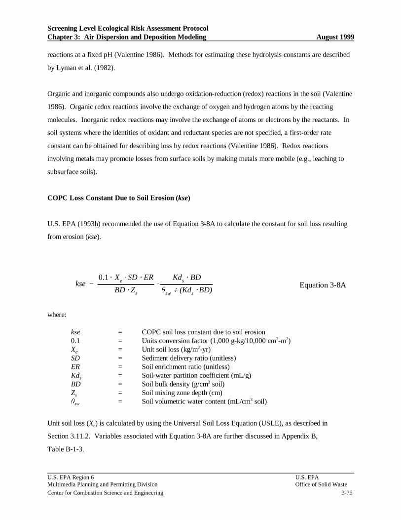
Screening Level Ecological Risk Assessment ProtocolChapter 3: Air Dispersion and Deposition Modeling August 1999
U.S. EPA Region 6 U.S. EPAMultimedia Planning and Permitting Division Office of Solid WasteCenter for Combustion Science and Engineering 3-75
kse '
0.1 @ Xe @ SD @ ER
BD @ Zs
@
Kds @ BD
sw % (Kds @ BD)Equation 3-8A
reactions at a fixed pH (Valentine 1986). Methods for estimating these hydrolysis constants are described
by Lyman et al. (1982).
Organic and inorganic compounds also undergo oxidation-reduction (redox) reactions in the soil (Valentine
1986). Organic redox reactions involve the exchange of oxygen and hydrogen atoms by the reacting
molecules. Inorganic redox reactions may involve the exchange of atoms or electrons by the reactants. In
soil systems where the identities of oxidant and reductant species are not specified, a first-order rate
constant can be obtained for describing loss by redox reactions (Valentine 1986). Redox reactions
involving metals may promote losses from surface soils by making metals more mobile (e.g., leaching to
subsurface soils).
COPC Loss Constant Due to Soil Erosion (kse)
U.S. EPA (1993h) recommended the use of Equation 3-8A to calculate the constant for soil loss resulting
from erosion (kse).
where:
kse = COPC soil loss constant due to soil erosion0.1 = Units conversion factor (1,000 g-kg/10,000 cm2-m2)Xe = Unit soil loss (kg/m2-yr)SD = Sediment delivery ratio (unitless)ER = Soil enrichment ratio (unitless)Kds = Soil-water partition coefficient (mL/g)BD = Soil bulk density (g/cm3 soil)Zs = Soil mixing zone depth (cm)
sw = Soil volumetric water content (mL/cm3 soil)
Unit soil loss (Xe) is calculated by using the Universal Soil Loss Equation (USLE), as described in
Section 3.11.2. Variables associated with Equation 3-8A are further discussed in Appendix B,
Table B-1-3.

Screening Level Ecological Risk Assessment ProtocolChapter 3: Air Dispersion and Deposition Modeling August 1999
U.S. EPA Region 6 U.S. EPAMultimedia Planning and Permitting Division Office of Solid WasteCenter for Combustion Science and Engineering 3-76
ksr '
RO
sw @ Zs
@
11 % Kds @ BD / sw
Equation 3-8B
U.S. EPA guidance (1994b and 1994l) have stated that all kse values are equal to zero. U.S. EPA (1994l)
stated that kse is equal to zero because of contaminated soil eroding onto and off of the site.
Consistent with earlier U.S. EPA guidance (1994b and 1994l) and U.S. EPA (1998c), U.S. EPA OSW
recommends that the constant for the loss of soil resulting from erosion (kse) should be set equal to zero.
Recommended Value for:COPC Loss Constant Due to Erosion (kse)
0
For additional information on addressing kse, U.S. EPA OSW recommends consulting the methodologies
described in U.S. EPA document, Methodology for Assessing Health Risks Associated with Multiple
Exposure Pathways to Combustor Emissions (U.S. EPA In Press). The use of kse values is also further
described in Appendix B, Table B-1-3.
COPC Loss Constant Due to Runoff (ksr)
Consistent with earlier U.S. EPA guidance (1993h; 1994l) and U.S. EPA (1998c), U.S. EPA OSW
recommends that Equation 3-8B be used to calculate the constant for the loss of soil resulting from surface
runoff (ksr). The use of this equation is further described in Appendix B, Table B-1-4.
Recommended Equation for Calculating:COPC Loss Constant Due to Runoff (ksr)
whereksr = COPC loss constant due to runoff (yrG1)RO = Average annual surface runoff from pervious areas (cm/yr)
sw = Soil volumetric water content (mL/cm3 soil)

Screening Level Ecological Risk Assessment ProtocolChapter 3: Air Dispersion and Deposition Modeling August 1999
U.S. EPA Region 6 U.S. EPAMultimedia Planning and Permitting Division Office of Solid WasteCenter for Combustion Science and Engineering 3-77
ksl 'P % I & RO & Ev
sw @ Zs @ [1.0 % ( BD @ Kds / sw)]Equation 3-8C
Zs = Soil mixing zone depth (cm)Kds = Soil-water partition coefficient (mL/g)BD = Soil bulk density (g/cm3 soil)
COPC Loss Constant Due to Leaching (ksl)
Consistent with earlier U.S. EPA guidance (1993h and 1994l) and U.S. EPA (1998c), U.S. EPA OSW
recommends that Equation 3-8C be used to calculate the COPC loss constant due to leaching (ksl). The
use of this equation is further described in Appendix B, Table B-1-5.
Recommended Equation for Calculating:COPC Loss Constant Due to Leaching (ksl)
whereksl = COPC loss constant due to leaching (yrG1)P = Average annual precipitation (cm/yr)I = Average annual irrigation (cm/yr)RO = Average annual surface runoff from pervious areas (cm/yr)Ev = Average annual evapotranspiration (cm/yr)
sw = Soil volumetric water content (mL/cm3 soil)Zs = Soil mixing zone depth (cm)Kds = Soil-water partition coefficient (mL/g)BD = Soil bulk density (g/cm3 soil)
Appendix B, Table B-1-5 further describes the variables associated with Equation 3-8C. The average
annual volume of water (P + I - RO - Ev) available to generate leachate is the mass balance of all water
inputs and outputs from the area under consideration.

Screening Level Ecological Risk Assessment ProtocolChapter 3: Air Dispersion and Deposition Modeling August 1999
U.S. EPA Region 6 U.S. EPAMultimedia Planning and Permitting Division Office of Solid WasteCenter for Combustion Science and Engineering 3-78
ksv '
3.1536 × 10⁷@ H
Zs @ Kds @ R @ Ta @ BD@
Da
Zs
@ 1 &
BD
s
& sw Equation 3-8D
COPC Loss Constant Due to Volatilization (ksv)
Semi-volatile and volatile COPCs emitted in high concentrations may become adsorbed to soil particles and
exhibit volatilization losses from soil. The loss of a COPC from the soil by volatilization depends on the
rate of movement of the COPC to the soil surface, the chemical vapor concentration at the soil surface, and
the rate at which vapor is carried away by the atmosphere (Jury 1986).
Consistent with U.S. EPA (In Press), U.S. EPA OSW recommends that Equation 3-8D be used to
calculate the constant for the loss of soil resulting from volatilization (ksv). The soil loss constant due to
volatilization (ksv) is based on gas equilibrium coefficients and gas phase mass transfer. The first order
decay constant, ksv, is obtained by adapting the Hwang and Falco equation for soil vapor phase diffusion
(Hwang and Falco 1986). The use of this equation is further described in Appendix B, Table B-1-6.
Recommended Equation for Calculating:COPC Loss Constant Due to Volatilization (ksv)
where
ksv = COPC loss constant due to volatization (yrG1)3.1536 × 107 = Units conversion factor (s/yr)H = Henry’s Law constant (atm-m3/mol)Zs = Soil mixing zone depth (cm)Kds = Soil-water partition coefficient (mL/g)R = Universal gas constant (atm-m3/mol-K)Ta = Ambient air temperature (K) = 298.1 KBD = Soil bulk density (g/cm3 soil)Da = Diffusivity of COPC in air (cm2/s)
sw = Soil volumetric water content (mL/cm3 soil)s = Solids particle density (g/cm3)
Appendix B, Table B-1-5 further describes the variables associated with Equation 3-8C. In cases where
high concentrations of volatile organic compounds are expected to be present in the soil, U.S. EPA OSW
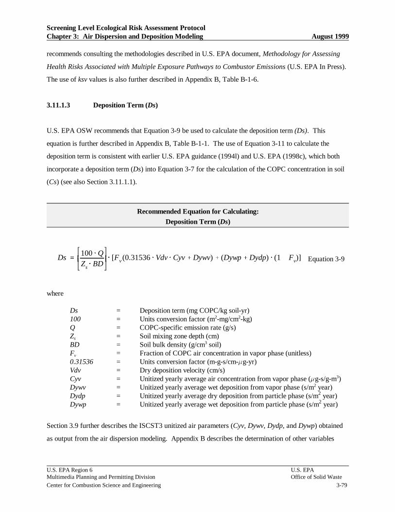
Screening Level Ecological Risk Assessment ProtocolChapter 3: Air Dispersion and Deposition Modeling August 1999
U.S. EPA Region 6 U.S. EPAMultimedia Planning and Permitting Division Office of Solid WasteCenter for Combustion Science and Engineering 3-79
Ds '
100 @ QZs @ BD
@ [Fv (0.31536 @ Vdv @ Cyv % Dywv) % (Dywp % Dydp) @ (1 & Fv)] Equation 3-9
recommends consulting the methodologies described in U.S. EPA document, Methodology for Assessing
Health Risks Associated with Multiple Exposure Pathways to Combustor Emissions (U.S. EPA In Press).
The use of ksv values is also further described in Appendix B, Table B-1-6.
3.11.1.3 Deposition Term (Ds)
U.S. EPA OSW recommends that Equation 3-9 be used to calculate the deposition term (Ds). This
equation is further described in Appendix B, Table B-1-1. The use of Equation 3-11 to calculate the
deposition term is consistent with earlier U.S. EPA guidance (1994l) and U.S. EPA (1998c), which both
incorporate a deposition term (Ds) into Equation 3-7 for the calculation of the COPC concentration in soil
(Cs) (see also Section 3.11.1.1).
Recommended Equation for Calculating:Deposition Term (Ds)
where
Ds = Deposition term (mg COPC/kg soil-yr)100 = Units conversion factor (m2-mg/cm2-kg)Q = COPC-specific emission rate (g/s)Zs = Soil mixing zone depth (cm)BD = Soil bulk density (g/cm3 soil)Fv = Fraction of COPC air concentration in vapor phase (unitless)0.31536 = Units conversion factor (m-g-s/cm-Fg-yr)Vdv = Dry deposition velocity (cm/s)Cyv = Unitized yearly average air concentration from vapor phase (Fg-s/g-m3)Dywv = Unitized yearly average wet deposition from vapor phase (s/m2 year)Dydp = Unitized yearly average dry deposition from particle phase (s/m2 year)Dywp = Unitized yearly average wet deposition from particle phase (s/m2 year)
Section 3.9 further describes the ISCST3 unitized air parameters (Cyv, Dywv, Dydp, and Dywp) obtained
as output from the air dispersion modeling. Appendix B describes the determination of other variables

Screening Level Ecological Risk Assessment ProtocolChapter 3: Air Dispersion and Deposition Modeling August 1999
U.S. EPA Region 6 U.S. EPAMultimedia Planning and Permitting Division Office of Solid WasteCenter for Combustion Science and Engineering 3-80
associated with Equation 3-9. The proper use of this equation is also further described in Appendix B,
Table B-1-1.
3.11.1.4 Site-Specific Parameters for Calculating Soil Concentration
As discussed in the previous sections, calculating the COPC concentration in soil (Cs) requires some
site-specific parameter values, which must be calculated or derived from available literature or site-specific
data. These site-specific parameters include the following:
C Soil mixing zone depth (Zs)
C Soil bulk density (BD)
C Available water (P + I - RO - Ev)
C Soil volumetric water content (θsw)
Determination of values for these parameters is further described in the following subsections, and in
Appendix B.
Soil Mixing Zone Depth (Zs)
When exposures to COPCs in soils are modeled, the depth of contamination is important in calculating the
appropriate soil concentration. Due to leaching and physical disturbance (e.g., tilling) COPCs may migrate
deeper in the soil in for some areas. Therefore, the value for the depth of soil contamination, or soil mixing
zone depth (Zs), used in modeling ecological risk should be considered specific to tilled (e.g., large plowed
field) or untilled soil areas.
In general, previous U.S. EPA combustion risk assessment guidance (1990a) has estimated that if the area
under consideration is tilled or mechanically disturbed, the soil mixing zone depth is about 10 to
20 centimeters depending on local conditions and the equipment used. If soil is not moved, COPCs are
assumed to be retained in the shallower, upper soil layer. In this case, earlier U.S. EPA guidances (U.S.
EPA 1990a; U.S. EPA 1993h) have typically recommended a value of 1 centimeter.

Screening Level Ecological Risk Assessment ProtocolChapter 3: Air Dispersion and Deposition Modeling August 1999
U.S. EPA Region 6 U.S. EPAMultimedia Planning and Permitting Division Office of Solid WasteCenter for Combustion Science and Engineering 3-81
Consistent with earlier U.S. EPA guidance (1990a) and U.S. EPA (1998c), U.S. EPA OSW recommends
the following values for the soil mixing zone depth (Zs).
Recommended Values for:Soil Mixing Zone Depth (Zs)
1 cm - untilled20 cm - tilled
Soil Bulk Density (BD)
BD is the ratio of the mass of soil to its total volume. This variable is affected by the soil structure, type,
and moisture content (Hillel 1980). Consistent with U.S. EPA (1990a; 1994b) and information presented
in Hoffman and Baes (1979), U.S. EPA OSW recommends the following value for the soil dry bulk density
(BD).
Recommended Value for:Soil Dry Bulk Density (BD)
1.50 g/cm3 soil
For determination of actual field values specific to a specified location at a site, U.S. EPA (1994l)
recommended that wet soil bulk density be determined by weighing a thin-walled, tube soil sample (e.g., a
Shelby tube) of known volume and subtracting the tube weight (ASTM Method D2937). Moisture content
can then be calculated (ASTM Method 2216) to convert wet soil bulk density to dry soil bulk density.
Available Water (P + I - RO - Ev)
The average annual volume of water available (P + I - RO - Ev) for generating leachate is the mass balance
of all water inputs and outputs from the area under consideration. A wide range of values for these
variables may apply in the various U.S. EPA regions.

Screening Level Ecological Risk Assessment ProtocolChapter 3: Air Dispersion and Deposition Modeling August 1999
U.S. EPA Region 6 U.S. EPAMultimedia Planning and Permitting Division Office of Solid WasteCenter for Combustion Science and Engineering 3-82
The average annual precipitation (P), irrigation (I), runoff (RO), and evapotranspiration (Ev) rates and
other climatological data may be obtained from either data recorded on site or from the Station Climatic
Summary for a nearby airport.
Meteorological parameters—such as the evapotranspiration rate and the runoff rate—may also be found in
resources such as Geraghty, Miller, van der Leeden, and Troise (1973). Surface runoff may also be
estimated by using the curve number equation developed by the U.S. Soil Conservation Service (U.S. EPA
1990a). U.S. EPA (1985b) cites isopleths of mean annual cropland runoff corresponding to various curve
numbers developed by Stewart, Woolhiser, Wischmeier, Caro, and Frere (1975). Curve numbers are
assigned to an area on the basis of soil type, land use or cover, and the hydrologic condition of the soil
(U.S. EPA 1990a).
Using these different references may introduce uncertainties and limitations. For example, Geraghty, van
der Leeden, and Troise (1973) present isopleths for annual surface water contributions that include
interflow and ground water recharge; these values should be adjusted downward to reflect surface runoff
only. U.S. EPA (1994b) recommends that these values be reduced by 50 percent.
Soil Volumetric Water Content ( sw)
The soil volumetric water content sw depends on the available water and the soil structure. A wide range
of values for these variables may apply in the various U.S. EPA regions. Consistent with earlier guidance
documents (U.S. EPA 1994b), U.S. EPA OSW recommends the following value for sw.
Recommended Value for:Soil Volumetric Water Content ( sw)
0.2 ml/cm3 soil
Additional information on soil water content is presented in Appendix B, specific to the equations in which
it is used.

Screening Level Ecological Risk Assessment ProtocolChapter 3: Air Dispersion and Deposition Modeling August 1999
U.S. EPA Region 6 U.S. EPAMultimedia Planning and Permitting Division Office of Solid WasteCenter for Combustion Science and Engineering 3-83
3.11.2 CALCULATION OF COPC CONCENTRATIONS IN SURFACE WATER AND
SEDIMENTS
COPC concentrations in surface water and sediments are calculated for all water bodies selected for
evaluation in the risk assessment. Mechanisms considered for determination of COPC loading of the water
column are:
(1) Direct deposition,
(2) Runoff from impervious surfaces within the watershed,
(3) Runoff from pervious surfaces within the watershed,
(4) Soil erosion over the total watershed,
(5) Direct diffusion of vapor phase COPCs into the surface water, and
(6) Internal transformation of compounds chemically or biologically.
Other potential mechanisms may require consideration on a case-by-case basis (e.g., tidal influences),
however, contributions from other potential mechanisms are assumed to be negligible in comparison with
those being evaluated.
The USLE and a sediment delivery ratio are used to estimate the rate of soil erosion from the watershed.
To evaluate the COPC loading to a water body from its associated watershed, the COPC concentration in
watershed soils should be calculated. As described in Section 3.11.1, the equation for COPC concentration
in soil includes a loss term that considers the loss of contaminants from the soil after deposition. These loss
mechanisms may all lower the soil concentration associated with a specific deposition rate.
Surface water concentration algorithms include a sediment mass balance, in which the amount of sediment
assumed to be buried and lost from the water body is equal to the difference between the amount of soil
introduced to the water body by erosion and the amount of suspended solids lost in downstream flow. As a
result, the assumptions are made that sediments do not accumulate in the water body over time, and an
equilibrium is maintained between the surficial layer of sediments and the water column. The total water
column COPC concentration is the sum of the COPC concentration dissolved in water and the COPC

Screening Level Ecological Risk Assessment ProtocolChapter 3: Air Dispersion and Deposition Modeling August 1999
U.S. EPA Region 6 U.S. EPAMultimedia Planning and Permitting Division Office of Solid WasteCenter for Combustion Science and Engineering 3-84
Figure 3-5 COPC Loading to the Water Body
concentration associated with suspended solids. Partitioning between water and sediment varies with the
COPC. The total concentration of each COPC is partitioned between the sediment and the water column.
Section 3.11.2.1 describes equations for computing COPC loading to a water body. Section 3.11.2.2
describes equations for computing total COPC concentration in a water body. Section 3.11.2.3 present the
equations for computing COPC concentration in water column and in sediment. These equations are also
presented and further defined in Appendix B.

Screening Level Ecological Risk Assessment ProtocolChapter 3: Air Dispersion and Deposition Modeling August 1999
U.S. EPA Region 6 U.S. EPAMultimedia Planning and Permitting Division Office of Solid WasteCenter for Combustion Science and Engineering 3-85
LT ' LDEP % Ldif % LRI % LR % LE % LI Equation 3-10
3.11.2.1 Total COPC Loading to a Water Body (LT)
Consistent with earlier U.S. EPA guidance (1994l) and U.S. EPA (1998c), U.S. EPA OSW recommends
the use of Equation 3-10 to calculate the total COPC load to a water body (LT). This equation is also
further described in Appendix B, Table B-2-1.
Recommended Equation for Calculating:Total COPC Load to the Water Body (LT)
where
LT = Total COPC load to the water body (including deposition, runoff, anderosion) (g/yr)
LDEP = Total (wet and dry) particle phase and wet vapor phase COPC directdeposition load to water body (g/yr)
Ldif = Vapor phase COPC diffusion (dry deposition) load to water body (g/yr)LRI = Runoff load from impervious surfaces (g/yr)LR = Runoff load from pervious surfaces (g/yr)LE = Soil erosion load (g/yr)LI = Internal transfer (g/yr)
Due to the limited data and uncertainty associated with the chemical or biological internal transfer, LI, of
compounds into daughter products, U.S. EPA OSW recommends a default value for this variable of zero.
However, if a permitting authority determines that site-specific conditions indicate calculation of internal
transfer should be considered, U.S. EPA OSW recommends following the methodologies described in U.S.
EPA NCEA document, Methodology for Assessing Health Risks Associated with Multiple Exposure
Pathways to Combustor Emissions (U.S EPA In Press). Calculation of each of the remaining variables
(LDEP, Ldif, LRI, LR, and LE) is discussed in the following subsections.

Screening Level Ecological Risk Assessment ProtocolChapter 3: Air Dispersion and Deposition Modeling August 1999
U.S. EPA Region 6 U.S. EPAMultimedia Planning and Permitting Division Office of Solid WasteCenter for Combustion Science and Engineering 3-86
LDEP ' Q @ [ Fv @ Dywwv % (1 & Fv ) @ Dytwp ] @ AW Equation 3-11
Total (Wet and Dry) Particle Phase and Wet Vapor Phase Contaminant Direct Deposition Load to
Water Body (LDEP)
Consistent with U.S. EPA (1994l) and U.S. EPA (1998c), U.S. EPA OSW recommends Equation 3-11 to
calculate the load to the water body from the direct deposition of wet and dry particles and wet vapors onto
the surface of the water body (LDEP). The equation is also further described in Appendix B, Table B-2-2.
Recommended Equation for Calculating:Total Particle Phase and Wet Vapor Phase Direct Deposition Load to Water Body (LDEP)
where
LDEP = Total (wet and dry) particle phase and wet vapor phase COPC directdeposition load to water body (g/yr)
Q = COPC emission rate (g/s)Fv = Fraction of COPC air concentration in vapor phase (unitless)Dywwv = Unitized yearly (water body and watershed) average wet deposition from
vapor phase (s/m2-yr)Dytwp = Unitized yearly (water body and watershed) average total (wet and dry)
deposition from vapor phase (s/m2-yr)AW = Water body surface area (m2)
Section 3.9 describes the unitized air parameters, Dywwv and Dywwv, obtained as output from the ISCST3
air dispersion modeling. The determination of water body surface area, Aw, is described in Chapter 4.
Appendix A-2 describes determination of the compound-specific parameter, Fv.

Screening Level Ecological Risk Assessment ProtocolChapter 3: Air Dispersion and Deposition Modeling August 1999
U.S. EPA Region 6 U.S. EPAMultimedia Planning and Permitting Division Office of Solid WasteCenter for Combustion Science and Engineering 3-87
Ldif 'Kv @ Q @ Fv @ Cywv @ AW @ 1×10&6
HR @ Twk
Equation 3-12
Diffusion Load to Water Body (Ldif)
Consistent with earlier U.S. EPA guidance (1994l) and U.S. EPA (1998c), U.S. EPA OSW recommends
using Equation 3-12 to calculate the dry vapor phase COPC diffusion load to the water body (Ldif). The
equation is described in detail in Appendix B, Table B-2-3.
Recommended Equation for Calculating:Vapor Phase COPC Diffusion (Dry Deposition) Load to Water Body (LDif)
where
Ldif = Vapor phase COPC diffusion (dry deposition) load to water body (g/yr)Kv = Overall COPC transfer rate coefficient (m/yr)Q = COPC emission rate (g/s)Fv = Fraction of COPC air concentration in vapor phase (unitless)Cywv = Unitized yearly (water body and watershed) average air concentration
from vapor phase (Fg-s/g-m3)AW = Water body surface area (m2)10-6 = Units conversion factor (g/Fg)H = Henry’s Law constant (atm-m3/mol)R = Universal gas constant (atm-m3/mol-K)Twk = Water body temperature (K)
The overall COPC transfer rate coefficient (Kv) is calculated by using the equation in Appendix B,
Table B-2-13. Consistent with previous U.S. EPA guidance (1994l; 1993h) and U.S. EPA (1998c), U.S.
EPA OSW recommends a water body temperature (Twk) of 298 K (or 25EC). Section 3.9 describes the
determination of the modeled air parameter, Cywv. The determination of water body surface area, Aw, is
described in Chapter 4. Appendix A-2 describes determination of compound-specific parameters, Fv and
H.

Screening Level Ecological Risk Assessment ProtocolChapter 3: Air Dispersion and Deposition Modeling August 1999
U.S. EPA Region 6 U.S. EPAMultimedia Planning and Permitting Division Office of Solid WasteCenter for Combustion Science and Engineering 3-88
LRI ' Q @ [ Fv @ Dywwv % (1.0 & Fv ) @ Dytwp ] @ AI Equation 3-13
Runoff Load from Impervious Surfaces (LRI)
In some watershed soils, a fraction of the wet and dry deposition in the watershed will be to impervious
surfaces. Dry deposition may accumulate and be washed off during rain events. Consistent with U.S. EPA
(1994l) and U.S. EPA (1998c), U.S. EPA OSW recommends the use of Equation 3-13 to calculate
impervious runoff load to a water body (LRI). The equation is also presented in Appendix B, Table B-2-4.
Recommended Equation for Calculating:Runoff Load from Impervious Surfaces (LRI)
where
LRI = Runoff load from impervious surfaces (g/yr)Q = COPC emission rate (g/s)Fv = Fraction of COPC air concentration in vapor phase (unitless)Dywwv = Unitized yearly (water body and watershed) average wet deposition from
vapor phase (s/m2-yr)Dytwp = Unitized yearly (water body and watershed) average total (wet and dry)
deposition from vapor phase (s/m2-yr)AI = Impervious watershed area receiving COPC deposition (m2)
Impervious watershed area receiving COPC deposition (AI) is the portion of the total effective watershed
area that is impervious to rainfall (i.e., roofs, driveways, streets, and parking lots) and drains to the water
body.
Runoff Load from Pervious Surfaces (LR)
Consistent with U.S. EPA (1994l) and U.S. EPA (1998c), U.S. EPA OSW recommends the use of
Equation 3-14 to calculate the runoff dissolved COPC load to the water body from pervious soil surfaces in
the watershed (LR). The equation is also presented in Appendix B, Table B-2-5.

Screening Level Ecological Risk Assessment ProtocolChapter 3: Air Dispersion and Deposition Modeling August 1999
U.S. EPA Region 6 U.S. EPAMultimedia Planning and Permitting Division Office of Solid WasteCenter for Combustion Science and Engineering 3-89
LR ' RO @ ( AL & AI ) @
Cs @ BD
sw % Kds @ BD@ 0.01 Equation 3-14
Recommended Equation for Calculating:Runoff Load from Pervious Surfaces (LR)
where
LR = Runoff load from pervious surfaces (g/yr)RO = Average annual surface runoff from pervious areas (cm/yr)AL = Total watershed area receiving COPC deposition (m2)AI = Impervious watershed area receiving COPC deposition (m2)Cs = COPC concentration in soil (in watershed soils) (mg COPC/kg soil)BD = Soil bulk density (g soil/cm3 soil)
sw = Soil volumetric water content (mL water/cm3 soil)Kds = Soil-water partition coefficient (cm3 water/g soil)0.01 = Units conversion factor (kg-cm2/mg-m2)
Appendix B describes the determination of site-specific parameters, RO, AL, AI, BD, and sw. The
calculation of the COPC concentration in soil (Cs) is discussed in Section 3.11.1 and Appendix B. Soil
bulk density (BD) and soil water content ( sw) are described in Section 3.11.1.4.
Soil Erosion Load (LE)
Consistent with U.S. EPA (1994l) and U.S. EPA (1998c), U.S. EPA OSW recommends the use of
Equation 3-15 to calculate soil erosion load (LE). The equation is also presented in Appendix B,
Table B-2-6.

Screening Level Ecological Risk Assessment ProtocolChapter 3: Air Dispersion and Deposition Modeling August 1999
U.S. EPA Region 6 U.S. EPAMultimedia Planning and Permitting Division Office of Solid WasteCenter for Combustion Science and Engineering 3-90
LE ' Xe @ ( AL & AI ) @ SD @ ER @
Cs @ Kds @ BD
sw % Kds @ BD@ 0.001 Equation 3-15
Recommended Equation for Calculating:Soil Erosion Load (LE)
where
LE = Soil erosion load (g/yr)Xe = Unit soil loss (kg/m2-yr)AL = Total watershed area (evaluated) receiving COPC deposition (m2)AI = Impervious watershed area receiving COPC deposition (m2)SD = Sediment delivery ratio (watershed) (unitless)ER = Soil enrichment ratio (unitless)Cs = COPC concentration in soil (in watershed soils) (mg COPC/kg soil)BD = Soil bulk density (g soil/cm3 soil)
sw = Soil volumetric water content (mL water/cm3 soil)Kds = Soil-water partition coefficient (mL water/g soil)0.001 = Units conversion factor (k-cm2/mg-m2)
Unit soil loss (Xe) and watershed sediment delivery ratio (SD) are calculated as described in the following
subsections and in Appendix B. COPC concentration in soil (Cs) is described in Section 3.11.1 and
Appendix B, Table B-1-1. Soil bulk density (BD) and soil water content ( sw) are described in
Section 3.11.1.4.

Screening Level Ecological Risk Assessment ProtocolChapter 3: Air Dispersion and Deposition Modeling August 1999
U.S. EPA Region 6 U.S. EPAMultimedia Planning and Permitting Division Office of Solid WasteCenter for Combustion Science and Engineering 3-91
Xe ' RF @ K @ LS @ C @ PF @
907.184047
Equation 3-16
Universal Soil Loss Equation - USLE
U.S. EPA OSW recommends that the universal soil loss equation (USLE), Equation 3-16, be used to
calculate the unit soil loss (Xe) specific to each watershed. This equation is further described in
Appendix B, Table B-2-7. Appendix B also describes determination of the site- and watershed-specific
values for each of the variables associated with Equation 3-16. The use of Equation 3-16 is consistent with
U.S. EPA (1994b; 1994l) and U.S. EPA (1998c).
Recommended Equation for Calculating:Unit Soil Loss (Xe)
whereXe = Unit soil loss (kg/m2-yr)RF = USLE rainfall (or erosivity) factor (yrG1)K = USLE erodibility factor (ton/acre)LS = USLE length-slope factor (unitless)C = USLE cover management factor (unitless)PF = USLE supporting practice factor (unitless)907.18 = Units conversion factor (kg/ton)4047 = Units conversion factor (m2/acre)
The USLE RF variable, which represents the influence of precipitation on erosion, is derived from data on
the frequency and intensity of storms. This value is typically derived on a storm-by-storm basis, but
average annual values have been compiled (U.S. Department of Agriculture 1982). Information on
determining site-specific values for variables used in calculating Xe is provided in U.S. Department of
Agriculture (U.S. Department of Agriculture 1997) and U.S. EPA guidance (U.S. EPA 1985b).
Refer to Appendix B, Table B-2-7 for additional discussion of the USLE.

Screening Level Ecological Risk Assessment ProtocolChapter 3: Air Dispersion and Deposition Modeling August 1999
U.S. EPA Region 6 U.S. EPAMultimedia Planning and Permitting Division Office of Solid WasteCenter for Combustion Science and Engineering 3-92
SD ' a @ (AL )&b Equation 3-17
Sediment Delivery Ratio (SD)
U.S. EPA OSW recommends the use of Equation 3-17 to calculate sediment delivery ratio (SD). The use
of this equation is further described in Appendix B, Table B-2-8.
Recommended Equation for Calculating:Sediment Delivery Ratio (SD)
where
SD = Sediment delivery ratio (watershed) (unitless)a = Empirical intercept coefficient (unitless)b = Empirical slope coefficient (unitless)AL = Total watershed area (evaluated) receiving COPC deposition (m2)
The sediment delivery ratio (SD) for a large land area, a watershed or part of a watershed, can be
calculated, on the basis of the area of the watershed, by using an approach proposed by Vanoni (1975).
Accordingly, U.S. EPA (1993h) recommended the use of Equation 3-17 to calculate the sediment delivery
ratio.
According to Vanoni (1975), sediment delivery ratios vary approximately with the -0.125 power of the
drainage area. Therefore, the empirical slope coefficient is assumed to be equal to 0.125. An inspection of
the data presented by Vanoni (1975) indicates that the empirical intercept coefficient varies with the size of
the watershed, as illustrated in Appendix B, Table B-2-8.
AL is the total watershed surface area affected by deposition that drains to the body of water. A watershed
includes all of the land area that contributes water to a water body. In assigning values to the watershed
surface area affected by deposition, consideration should be given to (1) the distance from the stack, (2) the
location of the area affected by deposition fallout with respect to the water body, and (3) in the absence of

Screening Level Ecological Risk Assessment ProtocolChapter 3: Air Dispersion and Deposition Modeling August 1999
U.S. EPA Region 6 U.S. EPAMultimedia Planning and Permitting Division Office of Solid WasteCenter for Combustion Science and Engineering 3-93
Cwtot 'LT
Vfx @ fwc% kwt @ AW @ ( dwc % dbs )Equation 3-18
any deposition considerations, watershed hydrology. Total sediment in a water body may have originated
from watershed soils that are (or have the potential to be) both affected and unaffected by deposition of
combustion emissions. If a combustor is depositing principally on a land area that feeds a tributary of a
larger river system, consideration must be given to an “effective” area. An effective drainage area will
almost always be less than the watershed.
3.11.2.2 Total Water Body COPC Concentration (Cwtot)
U.S. EPA OSW recommends the use of Equation 3-18 to calculate total water body COPC concentration
(Cwtot). The total water body concentration includes both the water column and the bed sediment. The
equation is also presented in Appendix B, Table B-2-9.
Recommended Equation for Calculating:Total Water Body COPC Concentration (Cwtot)
where
Cwtot = Total water body COPC concentration (including water column and bedsediment) (g COPC/m3 water body)
LT = Total COPC load to the water body (including deposition, runoff, anderosion) (g/yr)
Vfx = Average volumetric flow rate through water body (m3/yr)fwc = Fraction of total water body COPC concentration in the water column
(unitless)kwt = Overall total water body COPC dissipation rate constant (yrG1)AW = Water body surface area (m2)dwc = Depth of water column (m)dbs = Depth of upper benthic sediment layer (m)
The total COPC load to the water body (LT)—including deposition, runoff, and erosion—is described in
Section 3.11.2.1 and Appendix B, Table B-2-1. The depth of the upper benthic layer (dbs), which
represents the portion of the bed that is in equilibrium with the water column, cannot be precisely specified;

Screening Level Ecological Risk Assessment ProtocolChapter 3: Air Dispersion and Deposition Modeling August 1999
U.S. EPA Region 6 U.S. EPAMultimedia Planning and Permitting Division Office of Solid WasteCenter for Combustion Science and Engineering 3-94
fwc '(1 % Kdsw @ TSS @ 1×10&6 ) @ dwc / dz
(1% Kdsw @ TSS @ 1×10&6 ) @ dwc / dz % ( bs% Kdbs @ BS ) @ dbs /dz
Equation 3-19
fbs ' 1 & fwc Equation 3-20
however, U.S. EPA (1993h) recommended values ranging from 0.01 to 0.05. Consistent with U.S. EPA
(1994l; 1998c), U.S. EPA OSW recommends a default value of 0.03, which represents the midpoint of the
specified range. Issues related to the remaining parameters are summarized in the following subsections.
Fraction of Total Water Body COPC Concentration in the Water Column (fwc) and Benthic Sediment
(fbs)
Consistent with U.S. EPA (1998c), U.S. EPA OSW recommends using Equation 3-19 to calculate fraction
of total water body COPC concentration in the water column (fwc), and Equation 3-20 to calculate fraction
of total water body contaminant concentration in benthic sediment (fbs). The equations are also presented in
Appendix B, Table B-2-10.
Recommended Equation for Calculating:Fraction of Total Water Body COPC Concentration in
the Water Column (fwc) and Benthic Sediment (fbs)
where
fwc = Fraction of total water body COPC concentration in the water column(unitless)
fbs = Fraction of total water body COPC concentration in benthic sediment(unitless)
Kdsw = Suspended sediments/surface water partition coefficient (L water/kgsuspended sediment)
TSS = Total suspended solids concentration (mg/L)1 x 10-6 = Units conversion factor (kg/mg)dz = Total water body depth (m)
bs = Bed sediment porosity (Lwater/Lsediment)

Screening Level Ecological Risk Assessment ProtocolChapter 3: Air Dispersion and Deposition Modeling August 1999
U.S. EPA Region 6 U.S. EPAMultimedia Planning and Permitting Division Office of Solid WasteCenter for Combustion Science and Engineering 3-95
TSS '
Xe @ (AL&AI) @ SD @ 1x10 3
Vfx% Dss @ AW
Equation 3-21
Kdbs = Bed sediment/sediment pore water partition coefficient (L water/kg bottomsediment)
BS = Benthic solids concentration (g/cm3 [equivalent to kg/L])dwc = Depth of water column (m)dbs = Depth of upper benthic sediment layer (m)
U.S. EPA (1993h) and NC DEHNR (1997) recommended the use of Equations 3-19 and 3-20 to calculate
the fraction of total water body concentration occurring in the water column (fwc) and the bed sediments
(fbs). The partition coefficient Kdsw describes the partitioning of a contaminant between sorbing material,
such as soil, surface water, suspended solids, and bed sediments (see Appendix A-2). NC DEHNR (1997)
also recommended adding the depth of the water column to the depth of the upper benthic layer (dwc + dbs)
to calculate the total water body depth (dz).
NC DEHNR (1997) recommended a default total suspended solids (TSS) concentration of 10 mg/L, which
was adapted from U.S. EPA (1993h). However, due to variability in water body specific values for this
variable, U.S. EPA OSW recommends the use of water body-specific measured TSS values representative
of long-term average annual values for the water body of concern. Average annual values for TSS are
generally expected to be in the range of 2 to 300 mg/L; with additional information on anticipated TSS
values available in the U.S. EPA NCEA document, Methodology for Assessing Health Risks Associated
with Multiple Exposure Pathways to Combustor Emissions (U.S. EPA In Press).
If measured data is not available, or of unacceptable quality, a calculated TSS value can be obtained for
non-flowing water bodies using Equation 3-21.
where
TSS = Total suspended solids concentration (mg/L)Xe = Unit soil loss (kg/m2-yr)AL = Total watershed area (evaluated) receiving COPC deposition (m2)AI = Impervious watershed area receiving COPC deposition (m2)

Screening Level Ecological Risk Assessment ProtocolChapter 3: Air Dispersion and Deposition Modeling August 1999
U.S. EPA Region 6 U.S. EPAMultimedia Planning and Permitting Division Office of Solid WasteCenter for Combustion Science and Engineering 3-96
bs ' 1 & BS
s
SD = Sediment delivery ratio (watershed) (unitless)Vfx = Average volumetric flow rate through water body (value should be 0 for
quiescent lakes or ponds) (m3/yr)Dss = Suspended solids deposition rate (a default value of 1,825 for quiescent
lakes or ponds) (m/yr)AW = Water body surface area (m2)
The default value of 1,825 m/yr provided for Dss is characteristic of Stoke’s settling velocity for an
intermediate (fine to medium) silt.
Also, to evaluate the appropriateness of watershed-specific values (specific for non-flowing water bodies)
used in calculating the unit soil loss (Xe), as described in Section 3.11.2.1 and Appendix B, the water-body
specific measured TSS value should be compared to the calculated TSS value obtained using Equation 3-21.
If the measured and calculated TSS values differ significantly, parameter values used in calculating Xe
should be re-evaluated. This re-evaluation of TSS and Xe should also be conducted if the calculated TSS
value is outside of the normal range expected for average annual measured values, as discussed above.
Bed sediment porosity (bs) can be calculated from the benthic solids concentration by using the following
equation (U.S. EPA 1993h):
wherebs = Bed sediment porosity (Lwater/Lsediment)s = Bed sediment density (kg/L)
BS = Benthic solids concentration (kg/L)
U.S. EPA OSW recommends the following default value for bed sediment porosity (bs), which was
adapted from U.S. EPA (1993h) and U.S. EPA (1998c):

Screening Level Ecological Risk Assessment ProtocolChapter 3: Air Dispersion and Deposition Modeling August 1999
U.S. EPA Region 6 U.S. EPAMultimedia Planning and Permitting Division Office of Solid WasteCenter for Combustion Science and Engineering 3-97
kwt ' fwc @ kv % fbs @ kb Equation 3-22
Recommended Value for:Bed Sediment Porosity ( bs)
bs = 0.6 Lwater/Lsediment
(assuming s = 2.65 kg/L [bed sediment density] and BS = 1 kg/L [benthic solids concentration])
Values for the benthic solids concentration (BS) and depth of upper benthic sediment layer (dbs) range from
0.5 to 1.5 kg/L and 0.01 to 0.05 meters, respectively. However, consistent with earlier U.S. EPA guidance
(1993h; 1994l) and U.S. EPA (1998c), 1 kg/L is a reasonable default for most applications of the benthic
solids concentration (BS), and 0.03 meter is the default depth of the upper benthic layer (dbs). The default
depth of 0.03 meters is based on the midpoint of the range presented above. The use of this equation is
further described in Appendix B, Table B-2-10.
Overall Total Water Body COPC Dissipation Rate Constant (kwt)
Consistent with U.S. EPA (1994l) and U.S. EPA (1998c), U.S. EPA OSW recommends the use of
Equation 3-22 to calculate the overall dissipation rate of COPCs in surface water, resulting from
volatilization and benthic burial. The equation is also presented in Appendix B, Table B-2-11.
Recommended Equation for Calculating:Overall Total Water Body COPC Dissipation Rate Constant (kwt)
where
kwt = Overall total water body dissipation rate constant (yrG1)fwc = Fraction of total water body COPC concentration in the water column
(unitless)kv = Water column volatilization rate constant (yrG1)fbs = Fraction of total water body COPC concentration in benthic sediment
(unitless)kb = Benthic burial rate constant (yrG1)

Screening Level Ecological Risk Assessment ProtocolChapter 3: Air Dispersion and Deposition Modeling August 1999
U.S. EPA Region 6 U.S. EPAMultimedia Planning and Permitting Division Office of Solid WasteCenter for Combustion Science and Engineering 3-98
kv 'Kv
dz @ (1 % Kdsw @ TSS @ 1×10&6 )Equation 3-23
The variables fwc and fbs are discussed in the previous section, Equations 3-19 and 3-20, and calculated by
using the equations presented in Appendix B, Table B-2-10.
Water Column Volatilization Rate Constant (kv)
Consistent with U.S. EPA (1994l) and U.S. EPA (1998c), U.S. EPA OSW recommends using
Equation 3-23 to calculate water column volatilization rate constant. The equation is also presented in
Appendix B, Table B-2-12.
Recommended Equation for Calculating:Water Column Volatilization Rate Constant (kv)
where
kv = Water column volatilization rate constant (yrG1)Kv = Overall COPC transfer rate coefficient (m/yr)dz = Total water body depth (m)Kdsw = Suspended sediments/surface water partition coefficient (L water/kg
suspended sediments)TSS = Total suspended solids concentration (mg/L)1 x 10-6 = Units conversion factor (kg/mg)
Total water body depth (dz), suspended sediment and surface water partition coefficient (Kdsw), and total
suspended solids concentration (TSS), are previously described in this section. Kdsw is discussed in
Appendix A-2. The overall transfer rate coefficient (Kv) is described in the following subsection.
Overall COPC Transfer Rate Coefficient (Kv)
Volatile organic chemicals can move between the water column and the overlying air. The overall transfer
rate Kv, or conductivity, is determined by a two-layer resistance model that assumes that two “stagnant

Screening Level Ecological Risk Assessment ProtocolChapter 3: Air Dispersion and Deposition Modeling August 1999
U.S. EPA Region 6 U.S. EPAMultimedia Planning and Permitting Division Office of Solid WasteCenter for Combustion Science and Engineering 3-99
Kv ' K &1L % KG @
HR @ Twk
&1 &1
@
Twk& 293Equation 3-24
films” are bounded on either side by well-mixed compartments. Concentration differences serve as the
driving force for the water layer diffusion. Pressure differences drive the diffusion for the air layer. From
balance considerations, the same mass must pass through both films; the two resistances thereby combine
in series, so that the conductivity is the reciprocal of the total resistance.
Consistent with U.S. EPA (1993h) and U.S. EPA (1998c), U.S. EPA OSW recommends the use of
Equation 3-24 to calculate the overall transfer rate coefficient (Kv). The equation is also presented in
Appendix B, Table B-2-13.
Recommended Equation for Calculating:Overall COPC Transfer Rate Coefficient (Kv)
where
Kv = Overall COPC transfer rate coefficient (m/yr)KL = Liquid phase transfer coefficient (m/yr)KG = Gas phase transfer coefficient (m/yr)H = Henry’s Law constant (atm-m3/mol)R = Universal gas constant (atm-m3/mol-K)Twk = Water body temperature (K)
= Temperature correction factor (unitless)
The value of the conductivity Kv depends on the intensity of turbulence in the water body and the overlying
atmosphere. As Henry’s Law constant increases, the conductivity tends to be increasingly
influenced by the intensity of turbulence in water. Conversely, as Henry’s Law constant decreases, the
value of the conductivity tends to be increasingly influenced by the intensity of atmospheric turbulence.
The liquid and gas phase transfer coefficients, KL and KG, respectively, vary with the type of water body.
The liquid phase transfer coefficient (KL) is calculated by using Equations 3-25 and 3-26. The gas phase
transfer coefficient (KG) is calculated by using Equations 3-27 and 3-28.

Screening Level Ecological Risk Assessment ProtocolChapter 3: Air Dispersion and Deposition Modeling August 1999
U.S. EPA Region 6 U.S. EPAMultimedia Planning and Permitting Division Office of Solid WasteCenter for Combustion Science and Engineering 3-100
KL '
(1 × 10&4) @ Dw @ u
dz
@ 3.1536×10⁷ Equation 3-25
KL ' (C 0.5d @ W) @ ( a
w
)0.5@
k 0.33
z
@ (µw
w @Dw
)&0.67@ 3.1536×10⁷ Equation 3-26
Henry’s Law constants generally increase with increasing vapor pressure of a COPC and generally
decrease with increasing solubility of a COPC. Henry’s Law constants are compound-specific and are
presented in Appendix A-2. The universal ideal gas constant, R, is 8.205 × 10⁻⁵ atm-m3/mol-K, at 20EC.
The temperature correction factor (), which is equal to 1.026, is used to adjust for the actual water
temperature. Volatilization is assumed to occur much less readily in lakes and reservoirs than in moving
water bodies.
Liquid Phase Transfer Coefficient (KL)
Consistent with U.S. EPA (1998c), U.S. EPA OSW recommends using Equations 3-25 and 3-26 to
calculate liquid phase transfer coefficient. (KL). The use of these equations is further described in
Appendix B, Table B-2-14.
Recommended Equation for Calculating:Liquid Phase Transfer Coefficient (KL)
For flowing streams or rivers:
For quiescent lakes or ponds:
where
KL = Liquid phase transfer coefficient (m/yr)Dw = Diffusivity of COPC in water (cm2/s)u = Current velocity (m/s)1 × 10-4 = Units conversion factor (m2/cm2)dz = Total water body depth (m)Cd = Drag coefficient (unitless)W = Average annual wind speed (m/s)

Screening Level Ecological Risk Assessment ProtocolChapter 3: Air Dispersion and Deposition Modeling August 1999
U.S. EPA Region 6 U.S. EPAMultimedia Planning and Permitting Division Office of Solid WasteCenter for Combustion Science and Engineering 3-101
a = Density of air (g/cm3)w = Density of water (g/cm3)
k = von Karman’s constant (unitless)z = Dimensionless viscous sublayer thickness (unitless)
µw = Viscosity of water corresponding to water temperature (g/cm-s)3.1536 x 107 = Units conversion factor (s/yr)
For a flowing stream or river, the transfer coefficients are controlled by flow-induced turbulence. For these
systems, the liquid phase transfer coefficient is calculated by using Equation 3-25, which is the O’Connor
and Dobbins (1958) formula, as presented in U.S. EPA (1993h).
For a stagnant system (quiescent lake or pond), the transfer coefficient is controlled by wind-induced
turbulence. For quiescent lakes or ponds, the liquid phase transfer coefficient can be calculated by using
Equation 3-26 (O’Connor 1983; U.S. EPA 1993h).
The total water body depth (dz) for liquid phase transfer coefficients is discussed previously in this section.
Consistent with U.S. EPA (1994l) and U.S. EPA (1998c), U.S. EPA OSW recommends the use of the
following default values. These values are further described in Appendix A-2:
(1) a diffusivity of chemical in water ranging (Dw) from 1.0 × 10G5 to 8.5 × 10⁻² cm2/s,
(2) a dimensionless viscous sublayer thickness (z) of 4,
(3) a von Karman’s constant (k) of 0.4,
(4) a drag coefficient (Cd) of 0.0011 which was adapted from U.S. EPA (1993h),
(5) a density of air (a) of 0.0012 g/cm3 at standard conditions (temperature = 20EC or 293 K,pressure = 1 atm or 760 millimeters of mercury) (Weast 1986),
(6) a density of water (w) of 1 g/cm3 (Weast 1986),
(7) a viscosity of water (µw) of a 0.0169 g/cm-s corresponding to water temperature(Weast 1986).

Screening Level Ecological Risk Assessment ProtocolChapter 3: Air Dispersion and Deposition Modeling August 1999
U.S. EPA Region 6 U.S. EPAMultimedia Planning and Permitting Division Office of Solid WasteCenter for Combustion Science and Engineering 3-102
KG ' 36500 m/yr Equation 3-27
KG ' (C 0.5d @ W) @
k 0.33
z
@ (µa
a @ Da
)&0.67@ 3.1536×10⁷ Equation 3-28
Gas Phase Transfer Coefficient (KG)
U.S. EPA OSW recommends using Equations 3-27 and 3-28 to calculate gas phase transfer coefficient
(KG). The equation is also discussed in Appendix B, Table B-2-15.
Recommended Equation for Calculating:Gas Phase Transfer Coefficient (KG)
For flowing streams or rivers:
For quiescent lakes or ponds:
where
KG = Gas phase transfer coefficient (m/yr)Cd = Drag coefficient (unitless)W = Average annual wind speed (m/s)k = von Karman’s constant (unitless)
z = Dimensionless viscous sublayer thickness (unitless)µa = Viscosity of air corresponding to air temperature (g/cm-s)
a = Density of air corresponding to water temperature (g/cm3)Da = Diffusivity of COPC in air (cm2/s)3.1536 x 107 = Units conversion factor (s/yr)
U.S. EPA (1993h) indicated that the rate of transfer of a COPC from the gas phase for a flowing stream or
river is assumed to be constant, in accordance with O’Connor and Dobbins (1958) (Equation 3-27).
For a stagnant system (quiescent lake or pond), the transfer coefficients are controlled by wind-induced
turbulence. For quiescent lakes or ponds, U.S. EPA OSW recommends that the gas phase transfer
coefficient be computed by using the equation presented in O’Connor (1983) (Equation 3-28).

Screening Level Ecological Risk Assessment ProtocolChapter 3: Air Dispersion and Deposition Modeling August 1999
U.S. EPA Region 6 U.S. EPAMultimedia Planning and Permitting Division Office of Solid WasteCenter for Combustion Science and Engineering 3-103
kb 'Xe @ AL @ SD @ 1×10³
& Vfx @ TSS
AW @ TSS@
TSS @ 1×10&6
BS @ dbs
Equation 3-29
Wb ' kb @ dbs Equation 3-30
Consistent with U.S. EPA (1994l) and U.S. EPA (1998c), U.S. EPA OSW recommends 1.81 x 10⁻⁴ g/cm-s
for the viscosity of air corresponding to air temperature.
Benthic Burial Rate Constant (kb)
U.S. EPA OSW recommends using Equation 3-29 to calculate benthic burial rate (kb). The equation is also
discussed in Appendix B, Table B-2-16.
Recommended Equation for Calculating:Benthic Burial Rate Constant (kb)
where
kb = Benthic burial rate constant (yrG1)Xe = Unit soil loss (kg/m2-yr)AL = Total watershed area (evaluated) receiving deposition (m2)SD = Sediment delivery ratio (watershed) (unitless)Vfx = Average volumetric flow rate through water body (m3/yr)TSS = Total suspended solids concentration (mg/L)AW = Water body surface area (m2)BS = Benthic solids concentration (g/cm3)dbs = Depth of upper benthic sediment layer (m)1 x 10G6 = Units conversion factor (kg/mg)1 x 103 = Units conversion factor (g/kg)
The benthic burial rate constant (kb), which is calculated in Equation 3-29, can also be expressed in terms
of the rate of burial (Wb):

Screening Level Ecological Risk Assessment ProtocolChapter 3: Air Dispersion and Deposition Modeling August 1999
U.S. EPA Region 6 U.S. EPAMultimedia Planning and Permitting Division Office of Solid WasteCenter for Combustion Science and Engineering 3-104
where
Wb = Rate of burial (m/yr)kb = Benthic burial rate constant (yrG1)dbs = Depth of upper benthic sediment layer (m)
According to U.S. EPA (1994l) and U.S. EPA (1998c), COPC loss from the water column resulting from
burial in benthic sediment can be calculated by using Equation 3-29. These guidance documents also
recommend a benthic solids concentration (BS) value ranging from 0.5 to 1.5 kg/L, which was adapted
from U.S. EPA (1993h). U.S. EPA OSW recommends the following default value for benthic solids
concentration (BS).
Recommended Default Value for:Benthic Solids Concentration (BS)
1.0 kg/L
The calculated value for kb should range from 0 to 1.0; with low kb values expected for water bodies
characteristic of no or limited sedimentation (rivers and fast flowing streams), and kb values closer to 1.0
expected for water bodies characteristic of higher sedimentation (lakes). This range of values is based on
the relation between the benthic burial rate and rate of burial expressed in Equation 3-30; with the depth of
upper benthic sediment layer held constant. For kb values calculated as a negative (water bodies with high
average annual volumetric flow rates in comparison to watershed area evaluated), a kb value of 0 should be
assigned for use in calculating the total water body COPC concentration (Cwtot) in Equation 3-18. If the
calculated kb value exceeds 1.0, re-evaluation of the parameter values used in calculating Xe should be
conducted.
3.11.2.3 Total COPC Concentration in Water Column (Cwctot)
U.S. EPA OSW recommends using Equation 3-31 to calculate total COPC concentration in water column
(Cwctot). The equation is also discussed in Appendix B, Table B-2-17.

Screening Level Ecological Risk Assessment ProtocolChapter 3: Air Dispersion and Deposition Modeling August 1999
U.S. EPA Region 6 U.S. EPAMultimedia Planning and Permitting Division Office of Solid WasteCenter for Combustion Science and Engineering 3-105
Cwctot ' fwc @ Cwtot @
dwc % dbs
dwc
Equation 3-31
Recommended Equation for Calculating:Total COPC Concentration in Water Column (Cwctot)
where
Cwctot = Total COPC concentration in water column (mg COPC/L water column)fwc = Fraction of total water body COPC concentration in the water column
(unitless)Cwtot = Total water body COPC concentration, including water column and bed
sediment (mg COPC/L water body)dwc = Depth of water column (m)dbs = Depth of upper benthic sediment layer (m)
The use of Equation 3-31 to calculate total COPC concentration in water column is consistent with U.S.
EPA (1994l; 1998c).
Total water body COPC concentration—including water column and bed sediment (Cwtot) and fraction of
total water body COPC concentration in the water column (fwc)—should be calculated by using
Equation 3-18 and Equation 3-19, respectively. Depth of upper benthic sediment layer (dbs) is discussed
previously.
Dissolved Phase Water Concentration (Cdw)
U.S. EPA OSW recommends the use of Equation 3-32 to calculate the concentration of COPC dissolved in
the water column (Cdw). The equation is discussed in detail in Appendix B, Table B-2-18.

Screening Level Ecological Risk Assessment ProtocolChapter 3: Air Dispersion and Deposition Modeling August 1999
U.S. EPA Region 6 U.S. EPAMultimedia Planning and Permitting Division Office of Solid WasteCenter for Combustion Science and Engineering 3-106
Cdw '
Cwctot
1 % Kdsw @ TSS @ 1×10&6 Equation 3-32
Recommended Equation for Calculating:Dissolved Phase Water Concentration (Cdw)
where
Cdw = Dissolved phase water concentration (mg COPC/L water)Cwctot = Total COPC concentration in water column (mg COPC/L water column)Kdsw = Suspended sediments/surface water partition coefficient (L water/kg
suspended sediment)TSS = Total suspended solids concentration (mg/L)1 x 10-6 = Units conversion factor (kg/mg)
The use of Equation 3-32 to calculate the concentration of COPC dissolved in the water column is
consistent with U.S. EPA (1994l; 1998c).
The total COPC concentration in water column (Cwctot) is calculated by using the Equation 3-31 (see also
Appendix B, Table B-2-17). The surface water partition coefficient (Kdsw) and total suspended solids
concentration (TSS) are discussed previously.
COPC Concentration in Bed Sediment (Csed)
U.S. EPA OSW recommends the use of Equation 3-33 to calculate COPC concentration in bed sediment
(Csed). The equation is also presented in Appendix B, Table B-2-19.

Screening Level Ecological Risk Assessment ProtocolChapter 3: Air Dispersion and Deposition Modeling August 1999
U.S. EPA Region 6 U.S. EPAMultimedia Planning and Permitting Division Office of Solid WasteCenter for Combustion Science and Engineering 3-107
Csed ' fbs @ Cwtot @
Kdbs
bs % Kdbs @ BS@
dwc % dbs
dbs
Equation 3-33
Recommended Equation for Calculating:COPC Concentration in Bed Sediment (Csed)
where
Csed = COPC concentration in bed sediment (mg COPC/kg sediment)fbs = Fraction of total water body COPC concentration in benthic sediment
(unitless)Cwtot = Total water body COPC concentration, including water column and bed
sediment (mg COPC/L water body)Kdbs = Bed sediment/sediment pore water partition coefficient (L COPC/kg water
body)bs = Bed sediment porosity (Lpore water/Lsediment)
BS = Benthic solids concentration (g/cm3)dwc = Depth of water column (m)dbs = Depth of upper benthic sediment layer (m)
The use of Equation 3-33 to calculate the COPC concentration in bed sediment is consistent with U.S. EPA
(1994l; 1998c).
The total water body COPC concentration—including water column and bed sediment (Cwtot) and the
fraction of total water body COPC concentration that occurs in the benthic sediment (fbs)—is calculated by
using Equations 3-18 and 3-20, respectively. The bed sediment and sediment pore water partition
coefficient (Kdbs) is discussed in Appendix A-2. Bed sediment porosity (bs), benthic solids concentration
(BS), depth of water column (dwc), and depth of upper benthic layer (dbs) are discussed previously.
3.11.3 CALCULATION OF COPC CONCENTRATIONS IN PLANTS
The concentration of COPCs in plants is assumed to occur by three possible mechanisms:
C Direct deposition of particles—wet and dry deposition of particle phase COPCsonto the exposed plant surfaces.
C Vapor transfer—uptake of vapor phase COPCs by plants through their foliage.

Screening Level Ecological Risk Assessment ProtocolChapter 3: Air Dispersion and Deposition Modeling August 1999
U.S. EPA Region 6 U.S. EPAMultimedia Planning and Permitting Division Office of Solid WasteCenter for Combustion Science and Engineering 3-108
Figure 3-6 COPC Concentration in Plants
C Root uptake—root uptake of COPCs available from the soil and their transfer tothe aboveground portions of the plant.
The total COPC concentration in terrestrial plants, CTP is calculated as a sum of contamination occurring
through all three of these mechanisms.

Screening Level Ecological Risk Assessment ProtocolChapter 3: Air Dispersion and Deposition Modeling August 1999
U.S. EPA Region 6 U.S. EPAMultimedia Planning and Permitting Division Office of Solid WasteCenter for Combustion Science and Engineering 3-109
Pd' 1,000 @Q @ (1&Fv) @ [Dydp% (Fw@Dywp)] @Rp @ [1.0&exp(&kp @Tp)] @0.12Yp @ kp
Equation 3-34
3.11.3.1 Calculating Plant Concentration Due to Direct Deposition (Pd)
Consitent with previous U.S. EPA guidance (1994l) and U.S. EPA (1998c), U.S. EPA OSW recommends
the use of Equation 3-34 to calculate COPC concentration in plants due to direct deposition. The use of
this equation is further described in Appendix B, Table B-3-1.
Recommended Equation for Calculating:Plant Concentration Due to Direct Deposition (Pd)
where
Pd = Plant concentration due to direct (wet and dry) deposition (mg COPC/kgWW)
1,000 = Units conversion factor (mg/g)Q = COPC emission rate (g/s)Fv = Fraction of COPC air concentration in vapor phase (unitless)Dydp = Unitized yearly average dry deposition from particle phase (s/m2-yr)Fw = Fraction of COPC wet deposition that adheres to plant surfaces (unitless)Dywp = Unitized yearly wet deposition from particle phase (s/m2-yr)Rp = Interception fraction of the edible portion of plant (unitless)kp = Plant surface loss coefficient (yrG1)Tp = Length of plant exposure to deposition per harvest of the edible portion of
the ith plant group (yr)012 = Dry weight to wet weight conversion factor (unitless)Yp = Yield or standing crop biomass of the edible portion of the plant
(productivity) (kg DW/m2)
Section 3.9 describes the use of the unitized air parameters, Dydp and Dywp, obtained as output from the
air dispersion modeling. Appendix A-3 describes determination of Fv. Appendix B describes
determination of Fw, Rp, kp, Tp, and Yp. The dry weight to wet weight conversion factor of 0.12 is based
on the average rounded value from the range of 80 to 95 percent water content in herbaceous plants and
nonwoody plant parts (Taiz at al. 1991).

Screening Level Ecological Risk Assessment ProtocolChapter 3: Air Dispersion and Deposition Modeling August 1999
U.S. EPA Region 6 U.S. EPAMultimedia Planning and Permitting Division Office of Solid WasteCenter for Combustion Science and Engineering 3-110
Pv ' Q @ Fv @ 0.12 @
Cyv @ Bv
aEquation 3-35
3.11.3.2 Calculating Plant Concentration Due to Air-to-Plant Transfer (Pv)
Consistent with U.S. EPA (1998c), U.S. EPA OSW recommends the use of Equation 3-35 to calculate the
plant concentration due to air-to-plant transfer (Pv). The use of this equation is further described in
Appendix B, Table B-3-2.
Recommended Equation for Calculating:Plant Concentration Due to Air-to-Plant Transfer (Pv)
where
Pv = Plant concentration due to air-to-plant transfer (mg COPC/kg WW)Q = COPC emission rate (g/s)Fv = Fraction of COPC air concentration in vapor phase (unitless)Cyv = Unitized yearly average air concentration from vapor phase (µg-s/g-m3)Bv = Air-to-plant biotransfer factor ([mg COPC/g DW plant]/[mg COPC/g
air]) (unitless)012 = Dry weight to wet weight conversion factor (unitless)
a = Density of air (g/m3)
Section 3.9 describes the use of the unitized air parameter, Cyv. Appendix A-3 describes determination of
the COPC-specific parameters, Fv and Bv. The dry weight to wet weight conversion factor of 0.12 is
based on the average rounded value from the range of 80 to 95 percent water content in herbaceous plants
and nonwoody plant parts (Taiz at al. 1991). Appendix B further describes use of Equation 3-35,
including determination of Fw and a.
3.11.3.3 Calculating Plant Concentration Due to Root Uptake (Pr)
Consistent with previous U.S. EPA guidance (1994g; 1994l; 1995h) and U.S. EPA (1998c), U.S. EPA
OSW recommends the use of Equation 3-36 to calculate the plant concentration due to root uptake (Pr).
The use of this equation is further described in Appendix B, Table B-3-3.

Screening Level Ecological Risk Assessment ProtocolChapter 3: Air Dispersion and Deposition Modeling August 1999
U.S. EPA Region 6 U.S. EPAMultimedia Planning and Permitting Division Office of Solid WasteCenter for Combustion Science and Engineering 3-111
Pr ' Cs @ BCFr @ 0.12 Equation 3-36
Recommended Equation for Calculating:Plant Concentration Due to Root Uptake (Pr)
where
Pr = Plant concentration due to root uptake (mg COPC/kg WW)BCFr = Plant-soil biotransfer factor (unitless)Cs = COPC concentration in soil (mg COPC/kg soil)012 = Dry weight to wet weight conversion factor (unitless)
Equation 3-36 is based on the soil-to-aboveground plant transfer approach developed by Travis and Arms
(1988). The dry weight to wet weight conversion factor of 0.12 is based on the average rounded value
from the range of 80 to 95 percent water content in herbaceous plants and nonwoody plant parts (Taiz at
al. 1991). Appendix A-3 describes determination of the COPC-specific parameter BCFr. Section 3.11.1
and Appendix B describe calculation of Cs.
3.12 REPLACING DEFAULT PARAMETER VALUES
As discussed in Chapter 1, default parameter values are provided in this guidance for numerous inputs to
the fate and transport modeling. After completing a risk assessment based on the default parameter values
recommended in this guidance, risk assessors may choose to investigate replacing default parameter values
with measured or published values if a more representative estimate of site-specific risk can be obtained.
Use of parameter values other than those specified in this guidance should always be clearly described in
the risk assessment report and work plan, and approved by the permitting authority. U.S. EPA OSW
recommends that requests to change default parameter values include the following information, as
appropriate:
1. An explanation of why the use of a measured or published value other than the defaultvalue is warranted (e.g., the default parameter value is based on data or studies at sites inthe northwestern U.S., but the facility is located in the southeast);
2. The supporting technical basis of the replacement parameter value, including readablecopies (printed in English) of any relevant technical literature or studies;

Screening Level Ecological Risk Assessment ProtocolChapter 3: Air Dispersion and Deposition Modeling August 1999
U.S. EPA Region 6 U.S. EPAMultimedia Planning and Permitting Division Office of Solid WasteCenter for Combustion Science and Engineering 3-112
3. The basis of the default parameter value, as understood by the requestor, includingreadable copies (printed in English) of the referenced literature or studies (if available);
4. A comparison of the weight-of-evidence between the competing studies (e.g., the proposedreplacement parameter value is based on a study that is more representative of siteconditions, a specific exposure setting being evaluated, or a more scientifically valid studythan the default parameter value, the proposed replacement parameter is based on theanalysis of 15 samples as opposed to 5 for the default parameter value, or the site-specificstudy used more stringent quality control/quality assurance procedures than the study uponwhich the default parameter value is based);
5. A description of other risk assessments or projects where the proposed replacementparameter value has been used, and how such risk assessments or projects are similar tothe risk assessment in consideration.