Chapter 3: A Quantative Basis for Design Real design tries to reach an optimal compromise between a...

Chapter 3: A Quantative Basis for DesignReal design tries to reach an optimal compromise between a number of thing

Execution time

Memory requirements

Implementation costs

Simplicity

Portability

Etc

Here try and form an understanding and some estimates of costs by creating performance models. Try and

Compare efficiency of different algorithms

Evaluate scalability

Identify bottlenecks and other inefficiences

BEFORE we put significant effort into implementation (coding).

Chapter 3: A Quantative Basis for Design

Goals:

Develop performance models

Evaluate scalability

Choose between different algorithms

Obtain empirical performance data and use to validate performance models

Understand how network topology affects communication performance

Account for these effects in models

Recognise and account for factors other than performance e.g. implementation costs

3.1 Defining PerformanceDefining “performance” is a complex issue:

e.g. weather forecasting

? Must be completed in a max time (e.g. within 4 hours) => execution time metric

? Fidelity must be maximised (how much comp can you do to make realistic in that time)

? Minimise implementation and hardware costs

? Reliability

? Scalability

e.g. parallel data base search

? Runs faster than existing sequential program

? Scalability is less critical (database not getting order of mag larger)

? Easily adaptable at later date (modularity)

? Needs to be built quickly to meet deadline (implementation costs)

e.g. image processing pipeline

? Metric not total time but rather no of images can process per second (throughput)

? Or time it takes to process a single image

? Things might need to react in ~ real time (sensor)

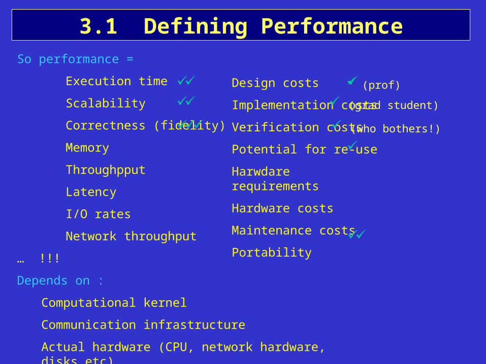
3.1 Defining PerformanceSo performance =

Execution time

Scalability

Correctness (fidelity)

Memory

Throughpput

Latency

I/O rates

Network throughput

… !!!

Depends on :

Computational kernel

Communication infrastructure

Actual hardware (CPU, network hardware, disks etc)

Design costs

Implementation costs

Verification costs

Potential for re-use

Harwdare requirements

Hardware costs

Maintenance costs

Portability

(grad student)

(who bothers!)

(prof)

3.2 Approaches to performance modellingThree common approaches to the characterisation of the performance of parallel algorithms:

Amdahl’s Law

Observations

Asymptotic analysis

We shall find that these are mostly inadequate for our purposes!

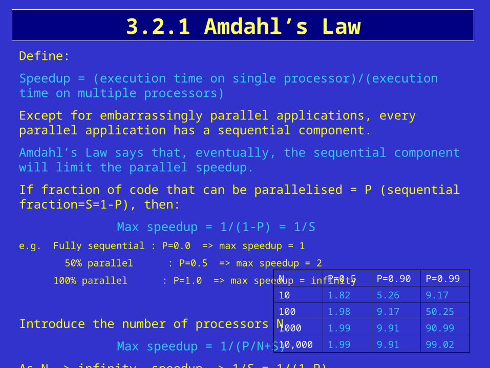
3.2.1 Amdahl’s LawDefine:

Speedup = (execution time on single processor)/(execution time on multiple processors)

Except for embarrassingly parallel applications, every parallel application has a sequential component.

Amdahl’s Law says that, eventually, the sequential component will limit the parallel speedup.

If fraction of code that can be parallelised = P (sequential fraction=S=1-P), then:

Max speedup = 1/(1-P) = 1/S

e.g. Fully sequential : P=0.0 => max speedup = 1

50% parallel : P=0.5 => max speedup = 2

100% parallel : P=1.0 => max speedup = infinity

Introduce the number of processors N

Max speedup = 1/(P/N+S)

As N -> infinity, speedup -> 1/S = 1/(1-P)

N P=0.5 P=0.90 P=0.99

10 1.82 5.26 9.17

100 1.98 9.17 50.25

1000 1.99 9.91 90.99

10,000 1.99 9.91 99.02

3.2.1 Amdahl’s Law (cont)

In early days of parallel computing, it was believed that this would limit the utility of parallel computing to a small number of specialised applications.

However, practical experience revealed that this was an inherently sequential way of thinking and it is of little relevance to real problems, if they are designed with parallel machines in mind from the start.

In general, dealing with serial bottlenecks is a matter of management of the parallel algorithm.

In the solution, some communication costs may be incurred that may limit scalability (or idle time or replicated computation)

Amdahl’s Law is relevant mainly where a program is parallelised incrementally

o Profile application to find the demanding components

o Adapt these components for parallel application

This partial or incremental parallelisation is only effective on small parallel machines. It looks like a “fork and join” => amenable to threads paradigm (e.g. openMP) and usable within small no. of multiprocessors of a node only.

Amdahl’s Law can be circumvented by designing complete parallel algorithms and trading communication to mask the serial components.

Furthermore, serial sections often remain constant in size whilst parallel sections increase with the problem size => serial fraction decreases with the problem size. This is a matter of scalability.

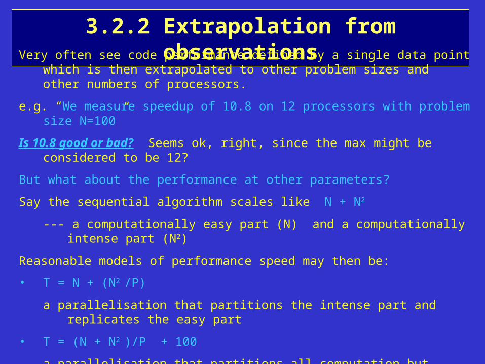
3.2.2 Extrapolation from observationsVery often see code performance defined by a single data point which is then extrapolated to

other problem sizes and other numbers of processors.

e.g. “We measure speedup of 10.8 on 12 processors with problem size N=100”

Is 10.8 good or bad? Seems ok, right, since the max might be considered to be 12?

But what about the performance at other parameters?

Say the sequential algorithm scales like N + N2

--- a computationally easy part (N) and a computationally intense part (N2)

Reasonable models of performance speed may then be:

• T = N + (N2 /P)

a parallelisation that partitions the intense part and replicates the easy part

• T = (N + N2 )/P + 100

a parallelisation that partitions all computation but introduces an overhead

• T = (N + N2 )/P + 0.6P2

a parallelisation that partitions all computation but introduces an overhead that depends on the partitioning

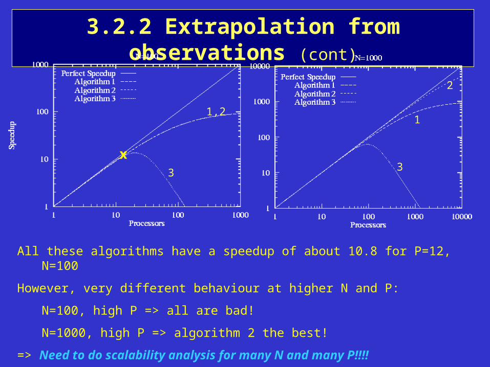
3.2.2 Extrapolation from observations (cont)

All these algorithms have a speedup of about 10.8 for P=12, N=100

However, very different behaviour at higher N and P:

N=100, high P => all are bad!

N=1000, high P => algorithm 2 the best!

=> Need to do scalability analysis for many N and many P!!!!

x

1,2

3

1

2

3

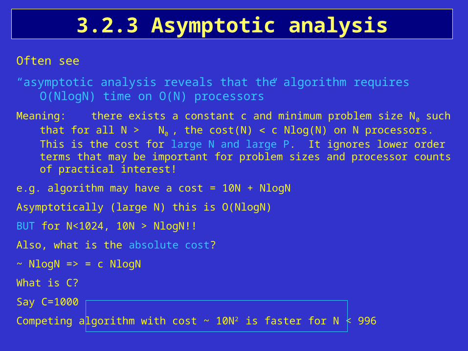
3.2.3 Asymptotic analysis

Often see

“asymptotic analysis reveals that the algorithm requires O(NlogN) time on O(N) processors”

Meaning: there exists a constant c and minimum problem size N0 such that for all N > N0 , the cost(N) c Nlog(N) on N processors. This is the cost for large N and large P. It ignores lower order terms that may be important for problem sizes and processor counts of practical interest!

e.g. algorithm may have a cost = 10N + NlogN

Asymptotically (large N) this is O(NlogN)

BUT for N<1024, 10N > NlogN!!

Also, what is the absolute cost?

~ NlogN => = c NlogN

What is C?

Say C=1000

Competing algorithm with cost ~ 10N2 is faster for N < 996

Summary: all useful concepts but inadequate!

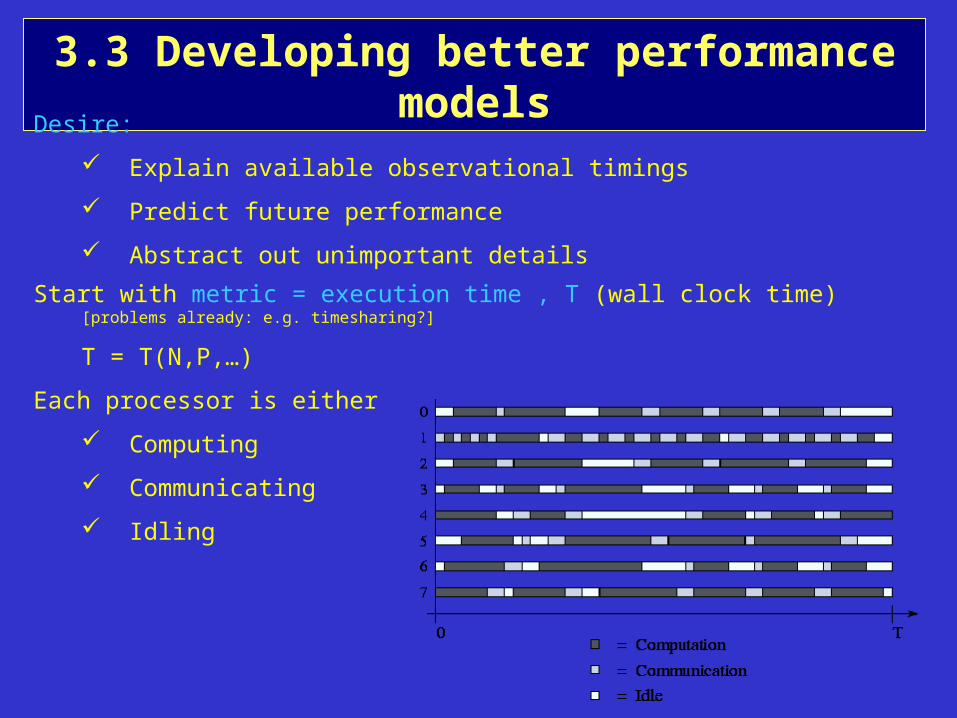
3.3 Developing better performance models

Desire:

Explain available observational timings

Predict future performance

Abstract out unimportant details

Start with metric = execution time , T (wall clock time) [problems already: e.g. timesharing?]

T = T(N,P,…)

Each processor is either

Computing

Communicating

Idling

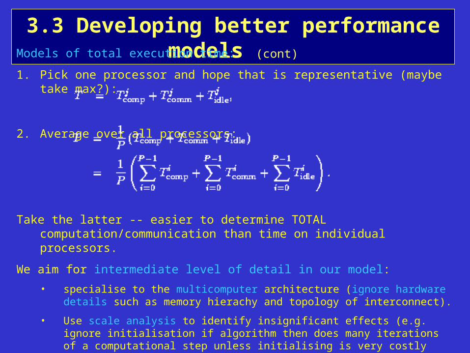
3.3 Developing better performance models (cont)

Models of total execution time:

1. Pick one processor and hope that is representative (maybe take max?):

2. Average over all processors:

Take the latter -- easier to determine TOTAL computation/communication than time on individual processors.

We aim for intermediate level of detail in our model:

• specialise to the multicomputer architecture (ignore hardware details such as memory hierachy and topology of interconnect).

• Use scale analysis to identify insignificant effects (e.g. ignore initialisation if algorithm then does many iterations of a computational step unless initialising is very costly etc)

• Use empirical studies to calibrate simple models rather than developing more complex models

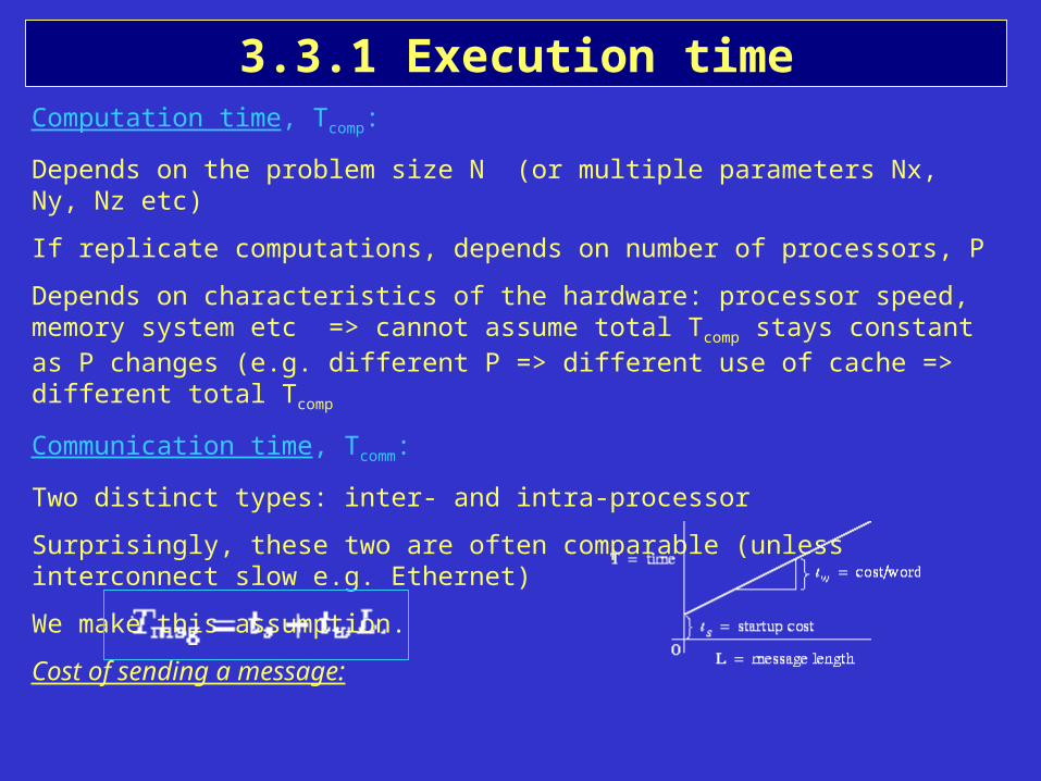
3.3.1 Execution timeComputation time, Tcomp:

Depends on the problem size N (or multiple parameters Nx, Ny, Nz etc)

If replicate computations, depends on number of processors, P

Depends on characteristics of the hardware: processor speed, memory system etc => cannot assume total Tcomp stays constant as P changes (e.g. different P => different use of cache => different total Tcomp

Communication time, Tcomm:

Two distinct types: inter- and intra-processor

Surprisingly, these two are often comparable (unless interconnect slow e.g. Ethernet)

We make this assumption.

Cost of sending a message:

ts = message startup time = time to initiate communication = LATENCY

tw = transfer time per word of data: determined by bandwith of channel

3.3.1 Execution time (cont)

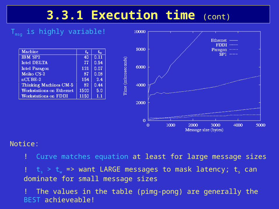
Tmsg is highly variable!

Notice:

! Curve matches equation at least for large message sizes

! ts > tw => want LARGE messages to mask latency; ts can dominate for small message sizes

! The values in the table (pimg-pong) are generally the BEST achieveable!


Idle time, Tidle:

Computation and communication time are explicitly specified in the parallel algorithm

Idle time is not => a little more complex. Depends on the ordering of operations.

Processor may be idle due to

1. Lack of computation

2. Lack of data: wait whilst remote data is computed and communicated

To reduce idle time:

For case 1: load-balance

For case 2: overlap computation and communication i.e. perform some computation or communication whilst waiting for remote date:

Multiple tasks on a processor: when one blocks, compute other. Issue: scheduling costs.

Interleave communications in amongst computation.


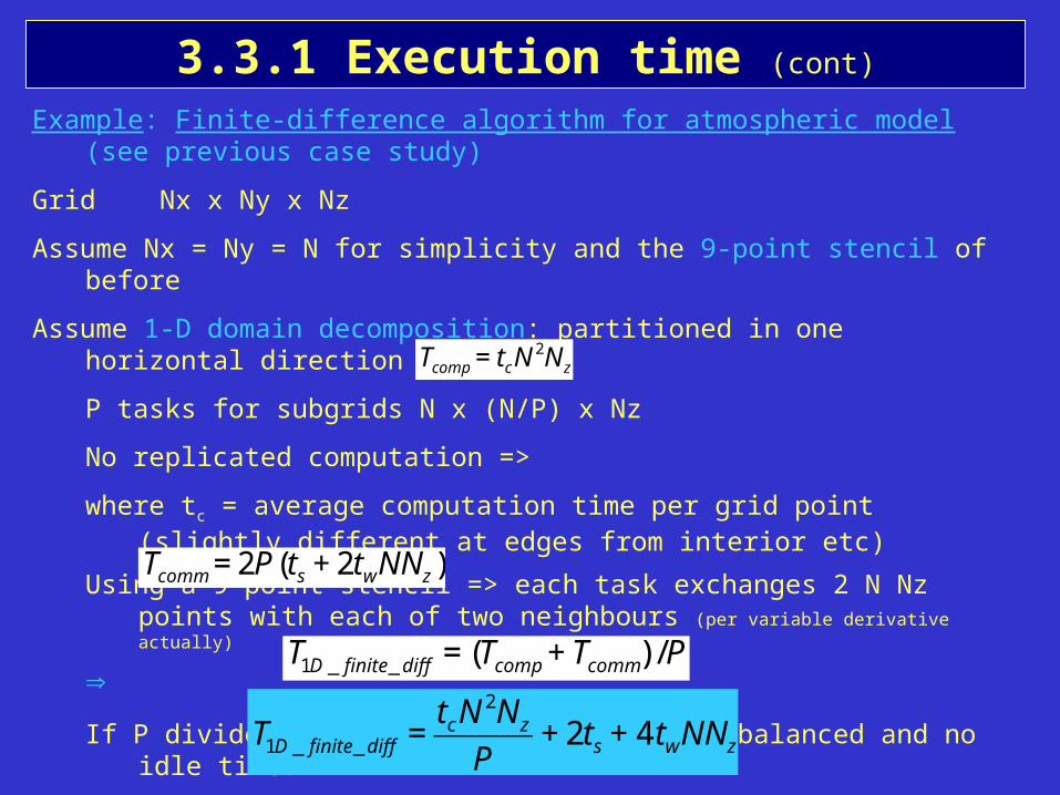
Example: Finite-difference algorithm for atmospheric model (see previous case study)

Grid Nx x Ny x Nz

Assume Nx = Ny = N for simplicity and the 9-point stencil of before

Assume 1-D domain decomposition: partitioned in one horizontal direction --

P tasks for subgrids N x (N/P) x Nz

No replicated computation =>

where tc = average computation time per grid point (slightly different at edges from interior etc)

Using a 9 point stencil => each task exchanges 2 N Nz points with each of two neighbours (per variable derivative actually)

If P divides N exactly, then assume load-balanced and no idle time:

€

T1D _ finite _ diff = (Tcomp + Tcomm ) /P

€

T1D _ finite _ diff =tcN

2Nz

P+ 2ts + 4 twNNz

€

Tcomp = tcN2Nz

€

Tcomm = 2P(ts + 2twNNz )

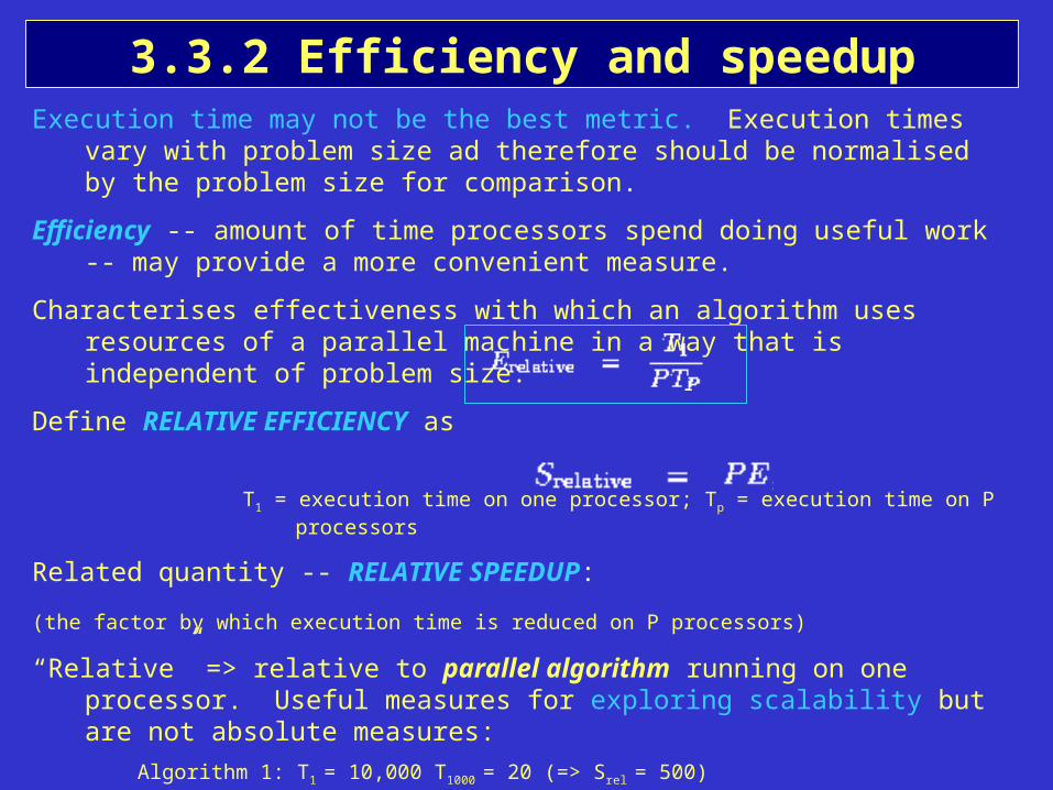
3.3.2 Efficiency and speedupExecution time may not be the best metric. Execution times vary with problem size ad

therefore should be normalised by the problem size for comparison.

Efficiency -- amount of time processors spend doing useful work -- may provide a more convenient measure.

Characterises effectiveness with which an algorithm uses resources of a parallel machine in a way that is independent of problem size.

Define RELATIVE EFFICIENCY as

T1 = execution time on one processor; Tp = execution time on P processors

Related quantity -- RELATIVE SPEEDUP:

(the factor by which execution time is reduced on P processors)

“Relative” => relative to parallel algorithm running on one processor. Useful measures for exploring scalability but are not absolute measures:

Algorithm 1: T1 = 10,000 T1000 = 20 (=> Srel = 500)

Algorithm 2: T1 = 1000 T1000 = 5 (=> Srel = 200)

Clearly, Algortithm 2 is better on 1000 processors despite Srel information!

Could do with absolute efficiency: use T1 of best uniprocessor algorithm? (we will not distinguish in general between absolute and relative here)

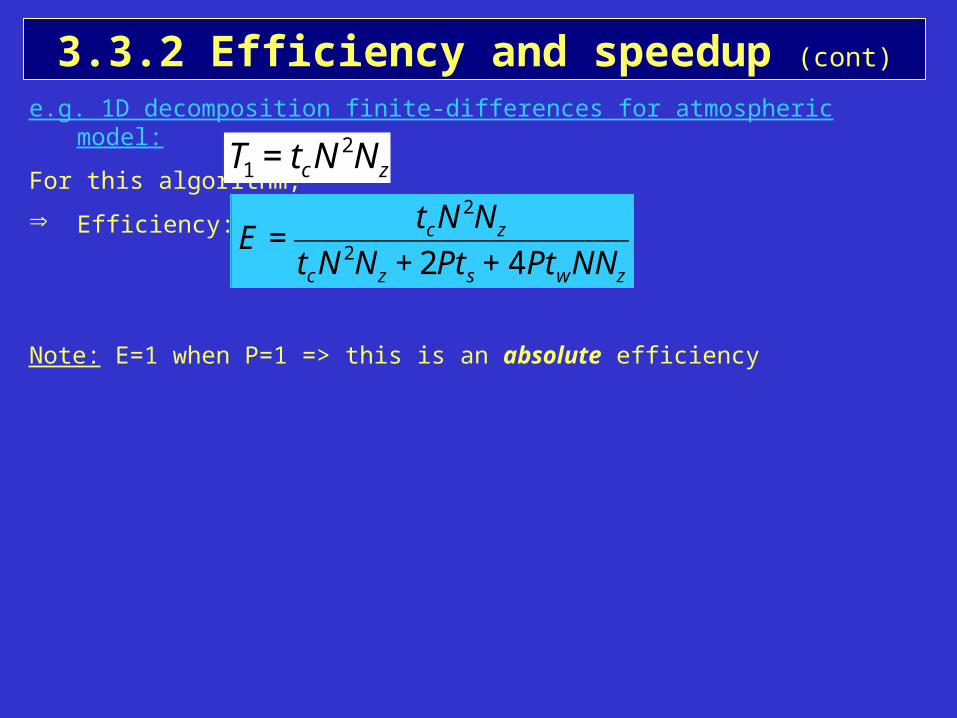
3.3.2 Efficiency and speedup (cont)

e.g. 1D decomposition finite-differences for atmospheric model:

For this algorithm,

Efficiency:

Note: E=1 when P=1 => this is an absolute efficiency

€

E =tcN

2Nz

tcN2Nz + 2Pts + 4PtwNNz

€

T1 = tcN2Nz

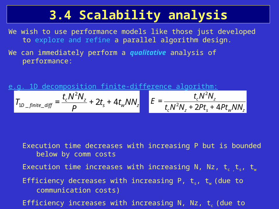
3.4 Scalability analysisWe wish to use performance models like those just developed to explore and refine a

parallel algorithm design.

We can immediately perform a qualitative analysis of performance:

e.g. 1D decomposition finite-difference algorithm:

Execution time decreases with increasing P but is bounded below by comm costs

Execution time increases with increasing N, Nz, tc ,ts, tw

Efficiency decreases with increasing P, ts, tw (due to communication costs)

Efficiency increases with increasing N, Nz, tc (due to masking of comm costs)

€

E =tcN

2Nz


€

T1D _ finite _ diff =tcN

2Nz

P+ 2ts + 4 twNNz

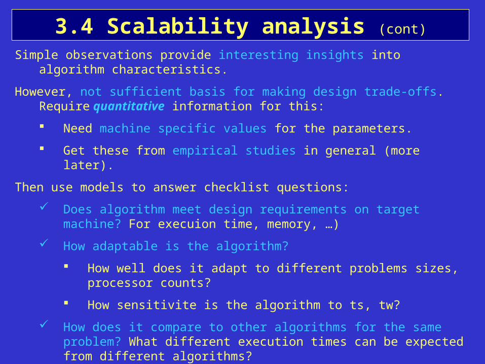
3.4 Scalability analysis (cont)

Simple observations provide interesting insights into algorithm characteristics.

However, not sufficient basis for making design trade-offs. Require quantitative information for this:

Need machine specific values for the parameters.

Get these from empirical studies in general (more later).

Then use models to answer checklist questions:

Does algorithm meet design requirements on target machine? For execuion time, memory, …)

How adaptable is the algorithm?

How well does it adapt to different problems sizes, processor counts?

How sensitivite is the algorithm to ts, tw?

How does it compare to other algorithms for the same problem? What different execution times can be expected from different algorithms?

Caution: these are of course huge simplifications of complex things (architecture my not be that close to multicomputer etc). Once algorithm implemented, validate models and adjust as necessary. BUT NOT A REASON FOR SKIPPING THIS STEP!


Scalability analysis can be performed in two ways:

1. Fixed problem size

2. Scaled problem size

3.4.1 Fixed problem size

In this mode can answer questions like:

How fast/efficiently can I solve a particular problem on a particular computer?

What is the largest number of processors I can use if I want to maintain an efficiency of great than 50%?

It is important to consider both T (execution time) and E (efficiency):

E will generally decrease monotonically with P

T will generally decrease monotonically with P

BUT T may actually increase with P if the performance model contains a term proportional to a positive power of P. In such cases, it may not be productive to use more than sime maximum number of processors for a particular problem size (and given machine parameters)


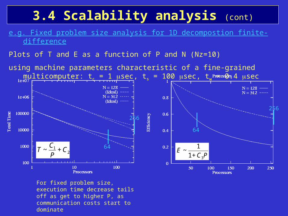
e.g. Fixed problem size analysis for 1D decompostion finite-difference

Plots of T and E as a function of P and N (Nz=10)

using machine parameters characteristic of a fine-grained multicomputer: tc = 1 sec, ts = 100 sec, tw = 0.4 sec

64

64

256

256

For fixed problem size, execution time decrease tails off as get to higher P, as communication costs start to dominate

€

T ~C1

P+ C2

€

E ~1

1+ C3P


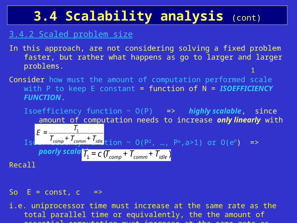
3.4.2 Scaled problem size

In this approach, are not considering solving a fixed problem faster, but rather what happens as go to larger and larger problems.

Consider how must the amount of computation performed scale with P to keep E constant = function of N = ISOEFFICIENCY FUNCTION.

Isoefficiency function ~ O(P) => highly scalable, since amount of computation needs to increase only linearly with P

Isoefficiency function ~ O(P2, …, Pa,a>1) or O(eP) => poorly scalable

Recall

So E = const, c =>

i.e. uniprocessor time must increase at the same rate as the total parallel time or equivalently, the the amount of essential computation must increase at the same rate as the overheads due to replicated computation, communication and idle time.

Scaled problems do not always make sense e.g. weather forecasting, image processng (sizes of computations may actually be fixed)

€

E =T1

Tcomp + Tcomm + Tidle

€

T1 = c(Tcomp + Tcomm + Tidle )

1


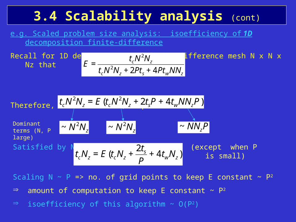
e.g. Scaled problem size analysis: isoefficiency of 1D decomposition finite-difference

Recall for 1D decomposition of finite-difference mesh N x N x Nz that

Therefore, for constant E, require

€

tcN2Nz = E(tcN

2Nz + 2tsP + 4 twNNzP)€

E =tcN

2Nz


€

~ N 2Nz

€

~ NNzP

€

~ N 2NzDominant terms (N, P large)

Satisfied by N=P

€

tcNz = E(tcNz +2ts

P+ 4 twNz)

(except when P is small)

Scaling N ~ P => no. of grid points to keep E constant ~ P2

amount of computation to keep E constant ~ P2

isoefficiency of this algorithm ~ O(P2)


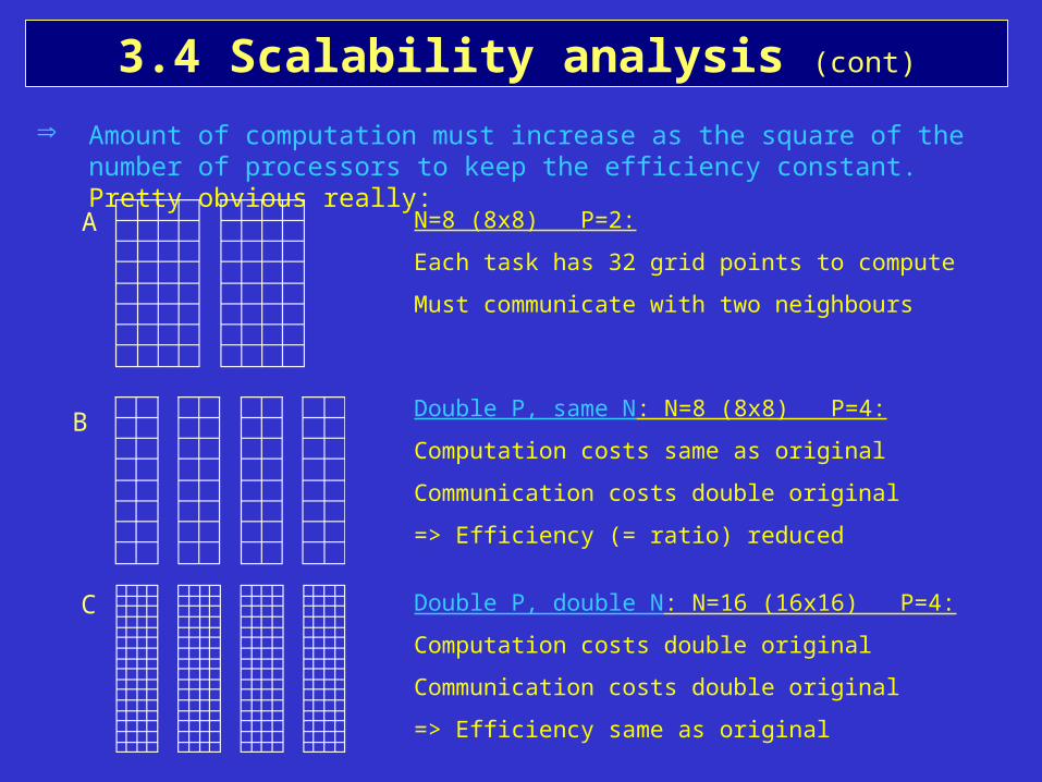
Amount of computation must increase as the square of the number of processors to keep the efficiency constant. Pretty obvious really:

N=8 (8x8) P=2:

Each task has 32 grid points to compute

Must communicate with two neighbours

Double P, same N: N=8 (8x8) P=4:

Computation costs same as original

Communication costs double original

=> Efficiency (= ratio) reduced

Double P, double N: N=16 (16x16) P=4:

Computation costs double original

Communication costs double original

=> Efficiency same as original

B

A

C


CLASS CASE STUDY:

Do scaled problem size analysis for isoefficiency of 2D decomposition finite-difference

Chapter 3: A Quantative Basis for Design Real design tries to reach an optimal compromise between a...

Documents

Transcript of Chapter 3: A Quantative Basis for Design Real design tries to reach an optimal compromise between a...