Chapter 24Information and Uncertainty

1.Arbitrage Pricing 2.Random Walk

Hypothesis 3.Variance Bounds4.Aggregating Information5.Risk Sharing

1. Arbitrage Pricing

The definition of competitive equilibrium implies that financial securities that have the same stochastic properties should command the same price

Payoff equivalence

There are some features of the solution to a market game that are evident without explicitly solving the game.

Perhaps the most important of these come from the notion of arbitrage, which is based on payoff equivalence.

We say two bundles of securities are payoff equivalent if the difference between their payoffs at the end of the game is zero with unit probability, that is for (almost) all possible histories of returns.

Arbitrage pricing

The optimal exploitation of arbitrage opportunities puts bounds on the best prices quoted in the limit order book of payoff equivalent portfolios.

Loosely speaking, arbitrage bundles of securities that offer the same payoffs should be traded at the same price.

More precisely, it should not be possible, by means of market orders alone, to sell one bundle of securities and purchase another payoff equivalent bundle and make a net profit.

2. The Random Walk Hypothesis

Suppose the objective of each trader is to maximize the expected value of his wealth. We investigate conditions under which the competitive equilibrium price will follow a random walk.

Maximizing expected value

For the purposes of this course segment we shall assume that traders maximize their expected value, an assumption that can plausibly applied to firms.

In the final segment on competitive equilibrium we shall assume that consumer exhibit risk aversion, and this leads them to take out insurance at actuarially unfair rates, and manage portfolios of financial assets with a view to looking beyond the expected return.

Currency exchange

Suppose U.S. export companies sporadically receive Euro and yuan injections from demanders for their goods in the E.U. between dates 0 and T.

Similarly European (and Chinese) exporters sporadically receive injections of dollars and yuan (euros) for their sales in the U.S. and China (Europe).

Export firms in each country also purchase domestic currency on the foreign exchange market between date 0 and T. At date T all export companies are liquidated and no further value is placed on holding foreign currency.

We assume the U.S. dollar is a dominant currency, meaning all currency prices are quoted in dollars.

Efficient markets hypothesis

We assume each export firm maximizes its expected dividend payments paid in domestic currency before the liquidation date T.

The liquidation value is unknown at all dates t < T, but as new information arrives about foreign trade throughout the trading phase, the traders become more informed about the value of foreign currency.

In competitive equilibrium the price of each exporter is the expected value of its dividend flow plus its liquidation value.

Therefore the exchange rates follow a random walk.

Proving the efficient markets hypothesis

Suppose the dollar price of yuan is lower in date t than its expected price in date s > t.

Chinese exporters buying yuan at date t are not maximizing their value, because the expected value of their companies would be higher if they postponed yen purchases until date s.

A symmetric argument applied to U.S. exporters explains why the the dollar price of yuan is not higher in date t than its expected price in date s > t.

Similar arguments apply to the dollar euro exchange market.

Market liquidity

The hypothesis that asset prices follow a random walk might be regarded as a test of liquidity.

In the previous example we may assume without loss of generality that there is continuous trading in the asset up until a common liquidation date T when the capitalized value of all the firms are recognized.

How would prices behave if consumers had limited opportunities to enter and exit the market, effectively segmenting the market into different time markets?

Illiquid markets

Suppose exporters face the threat of their foreign earnings being confiscated, or there are incomplete markets that limit savings and borrowing opportunities in domestic markets.

Then exporters might immediately capitalize their foreign earnings by converting them to domestic dividends and distributing them as dividends.

In this case successive prices in the foreign exchange market would exhibit mean reversion.

At the other extreme to the random walk observed in perfectly liquid market, prices in disconnected markets are independently distributed, and in a stationary environment, have the same conditional mean.

3. Variance Bounds

How well competitive equilibrium does aggregate knowledge demanders and suppliers have about tastes and technologies?

We first explore competitive equilibrium predictions in asset markets where all traders are symmetrically informed, and then turn to trading games with incomplete information.

Restrictions on higher order moments

It has been argued that the the random walk hypothesis is quite weak, and that there are other implications from rational behavior on price processes in liquid markets.

As rational consumers process information, this affects the variances of prices.

More specifically, variances of discounted summed dividend streams that condition on more information are larger than those which condition on less.

Some notationLet:

denote the summed value of future dividends from time s until time T, the liquidation date.

Also define:

as the competitive equilibrium asset price at time s, which is conditional on past dividend performance.

The competitive equilibrium price of the stock, , is based on less information than .

The next slide proves:

Intuitively, impounding information into prices creates variation that reflects updating in the asset’s value.

ps

p s t sT d t

p s Es t sT d t

ps

varps varps

Proving the inequalities implied by variance bounds

Since:

it follows that:

But and:

The result now follows directly.

ps ps ps ps

varp s varp s varp s p s 2covp s p s,p s

varps ps 0

covps ps,ps E

t sT d t Es

t sT d t Es

t sT d t E

t sT d t

0

4. Aggregating Information

How well competitive equilibrium does aggregate knowledge demanders and suppliers have about tastes and technologies?

We first explore competitive equilibrium predictions in asset markets where all traders are symmetrically informed, and then turn to trading games with incomplete information.

Incomplete information

In the trading games described above, all traders have the same information, and trade occurs because of differences in stochastic endowments and preferences.

In the remaining slides on this topic we investigate how differences in information between traders affect trading.

We will be particularly concerned with what competitive equilibrium predicts in trading games where there is incomplete information, and how seriously one should take those predictions.

The no-trade theorem

Suppose people have differential information about an asset they would all value the same way.

Will any trade take place?

Note that if one trader party benefits from the trading then the other party must lose.

Since all traders anticipate this, we thus establish that no trade occurs in competitive equilibrium, or for that matter any other solution to a (voluntary) trading mechanism, because of differences in information alone.

Competitive equilibrium and information

Competitive equilibrium economizes on the amount of information traders need to optimize their portfolios.

Indeed a peculiar feature of competitive equilibrium is that in some situations it fully reveals private information to those who are less informed about market conditions.

Private valuations in competitive equilibrium

A simple example illustrating how competitive equilibrium aggregates information is in a market where consumer valuations are identically and independently distributed, and aggregate supply is fixed.

Suppose no demander wants to consume more than one unit of the good, and each demander draws an identically and independently distributed random variable that determines their valuation for the first unit.

The competitive equilibrium price does not depend on whether each trader observes the valuations of the others. Hence every trader acts the same way as he would if he were fully informed about aggregate demand.

Fully revealing prices

Suppose there are N traders, and the nth trader receives a signal sn about the the state of the economy, where n = 1,2, . . ., N.In general, the competitive equilibrium price vector p depends on all the signals the traders receive.If, however, p is an invertible mapping of all the relevant information s available to traders, then every trader acts the same way as he would if he were fully informed.In this case p(s) has an inverse which we call f(p). Each trader realizes that seeing p is as good as seeing s.In the example above s is aggregate demand, and p is monotone increasing in s.

Differential information about product quality

Now suppose a component of each demander valuation is common, and traders have differential information about that component.

The more favorable the signal to the informed traders, the greater is their demand, and hence the higher is the market clearing price.

As in the previous example, uninformed traders compute their demands, deducing that if the market clearing price is p, then the common component is f(p). Thus informed traders cannot benefit from their superior information in competitive equilibrium.

Implications for trading mechanisms

Some economists have used this theoretical result to argue that markets are good at aggregating the information that traders have about the preferences of demanders and the technologies of suppliers.

Other economists have argued there is limited investment in acquiring new information relevant to suppliers and demanders, because those who use up resources to become better informed cannot recoup the benefit from their private information.

Both arguments implicitly assume that a competitive equilibrium accurately predicts price and resource allocations from trading.

When do competitive equilibrium prices hide information?

There are two scenarios when competitive equilibrium prices are not fully revealing:

1. The mapping from signals to prices p(s) is not invertible. That is, two or more values of a signal, s1 and s2, would yield the same fully revealing competitive equilibrium price if everyone observed the signal’s value, meaning pfr(s1) = pfr(s2).

2. Different units of the product are not identical, although they are traded on the same market, and these differences are observed by some but not all the traders.

Adding dimensions to uncertainty

The uninformed segment of the population can infer the true state in the previous example because a mapping exists from the competitive equilibrium price to the shock defining the product quality.

In our next example we introduce a second shock.

Those traders who observe one shock can infer the other from the competitive equilibrium price.

Those who observe neither can only form estimates of what both shocks are from the competitive equilibrium price.

Uncertain supply and quality

Now suppose that product quality is only known by some of the demanders, and the aggregate quantity supplied is also a random variable.

In this case an uninformed demander cannot infer product quality from the competitive equilibrium price, because a high price could indicate high demand from informed traders or low supply.

Informed demanders benefit from the fact that demand by uninformed traders is less than it would be if they were fully informed when product quality is high, depressing the price for high quality goods, and vice versa.

Differential information about heterogeneity across units

Suppose the quality of the individual units varies, and that traders are differentially informed it. What would competitive equilibrium theory predict about the price and quantity traded?

Since traders condition their individual demand and supply on their information, more informed traders gain at the expense of the less informed.

The prospect of being exploited by a well informed trader discourages a poorly informed player from trading.

The market for lemons

For example, consider a used car market.

Suppose there are less cars than commuter traders, and no one demands more than one car.

The valuation of a trader for owning one car is identically and independently distributed across the population.

The quality of each car is independently and identically distributed across the population. Each owner, but no one, else knows the quality of his car.

The amenity value from car travel is the product of the commuter’s valuation and the quality of the car he owns.

5. Risk Sharing

The final segment of this topic turns to portfolio management and asset pricing. Models of competitive equilibrium have been extensively applied in financial markets.

We investigate the role risk aversion plays in portfolio choice, as it applies to the relationship between financial returns of different assets, and the consumption profiles of investors.

Demand for financial assets

Individuals and households hold wealth in financial securities to defer consumption.

For example parents save for the education of their children, individuals save for retirement, and the wealthy bequest future generations with their largesse.

Half of the value of the stock market is held by a very small fraction of individuals. Nevertheless more than 50 percent of households hold financial securities of some form or other.

Collectively, these groups, including foreign investors, create the demand for financial securities.

Supply of financial assets The main financial securities are:

1. Stocks, bonds and their derivatives issued by corporations and private enterprises to finance their operations

2. Mortgage backed securities that bundle loans on housing stock

3. Bonds issued by governments (local, state and federal) to help finance their public expenditures

4. Fiat money or currency, and foreign exchange issued national governments, and managed by the banking system.

Risk sharing in a competitive equilibrium

If traders only cared about the mean return of an asset, it is hard to justify why assets could have different mean returns.

There is abundant evidence that assets have different mean returns, suggesting that traders care about other moments of the probability distribution apart from the first.

For example, suppose that traders are risk averse, rather than risk neutral. In this case they would seek to diversify their portfolio.

Risk and portfolio choice

Starting with the basic model of inter-temporal consumption smoothing, we derive the fundamental equation that determines how financial assets are priced in competitive equilibrium.

This leads into a discussion of how theories of risk sharing based on competitive equilibrium pricing can be tested using experimental methods.

Preferences under uncertainty about the timing of consumption

Consider the the lifetime utility of a consumer whose labor supply and wage income are determined outside the model:

where: is the period or year

is a subjective discount factor

is consumption in period t

is current utility, which we assume is concave increasing throughout its domain.

1

0

T

t tt cu

tt

cu

c

Tt

0

10

1,,2,1,0

Budget constraint

Suppose the person has assets, which can either consumed or invested in J financial securities:

where: is the amount of the jth security bought at the

beginning of period t

is the return on the jth security announced at the end of period t

J

j tjjttjt qqrc1 ,1

tj

tj

r

q

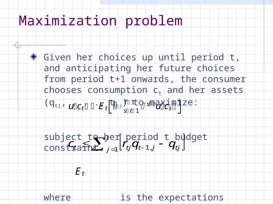
Maximization problem

Given her choices up until period t, and anticipating her future choices from period t+1 onwards, the consumer chooses consumption ct and her assets (qt1, . . ., qtJ) to maximize:

subject to her period t budget constraint

where is the expectations operator based on information at time t.

J

j tjjttjt qqrc1 ,1

uct E t s t 1T 1 s tucs

E t

Non-satiation in consumption

If u(ct) is strictly increasing, all wealth is consumed, all the budget constraints are met with strict equality, yielding the expression for consumption:

This implies we can express for consumption into the objective function, and reformulate the consumer investor’s problem as sequentially choosing the vector of assets to maximize:

ct j 1J rt 1,jq t 1,j q tj

q t1 , ,q tJ

u j 1J rt 1,jq t 1,j q tj E t

s t 1T 1 s tu

j 1J rs 1,jqs 1,j qs,j

The fundamental equation of portfolio choice

The interior first order condition requires that for each asset held by the consumer:

Substituting the definition of consumption back into the first order condition we obtain:

or

Asset return is discounted by the expected marginal rate of substitution between current and future consumption.

u j 1J rt 1,jq t 1,j q tj E t rtju

j 1J rtjq tj q t 1,j

u ct E trtju ct 1

E t rtj u c t 1 u c t

E trtjm t 1

Side conditions for not holding certain assets

Since u(c) is concave increasing it follows that if no units of the jth asset is held, that is:

then:

This equation says that the distribution of returns on the jth asset are too low to justify buying any units of the asset.

u ct E trtju ct 1

q tj 0

Market clearing conditions

For each trader a first order condition applies to each positively consumed asset; otherwise it is not held.

These conditions imply there is a solution to the asset allocation of each trader as a function of his asset endowment at the beginning of the period and the joint probability distribution governing asset returns.

To express the market clearing conditions, we temporarily superscript asset endowments and allocations for trader n.

Market clearing in competitive equilibrium means that every period the demand for each asset exactly offsets its supply:

n 1N rt 1,jq t 1,j

n q tjn 0

rt 1,jq t 1,jn

q tjn

The risk free rate

If a risk free (interest) rate called rt exists, it must satisfy the equation too:

or:

rt 1/E tm t

rtE tm t 1

Risk correctionsRecall from the definition of a covariance:

Dividing both sides of the equation by the expected value of the marginal rate of substitution yields

Using the formulas

in the equation above we now obtain the risk correction for the mean return on the jth asset :

covtrtj,m t E trtjm t E trtjE tm t

rt 1/E tm t E trtjm t 1

E trtj rt rtcovtrtj,m t

E trtj E trtjm t /E tm t covtrtj,m t /E tm t

The mean-variance frontier

From the risk correction formula for the mean return on the jth asset, we can write:

where is the correlation coefficient between mt and rjt, is the variance of rjt, and is the variance of mt.

Since the absolute value of every correlation coefficient is bounded by one, the following inequality must be satisfied in a competitive equilibrium:

E trtj rt rt jt mtcov tr tj ,mt

jt mt rt jt mt t

t

mt2 jt2

E tr tj r tr t jt mt