Chapter 22

On Exogeneity

David Kaplan

22.1. Introduction

When using linear statistical models to estimatesubstantive relationships, a distinction is made be-tween endogenous variables and exogenous variables.Alternative names for these variables are dependentand independent, or criterion and predictor. In the caseof multiple linear regression, one variable is desig-nated as the endogenous variable, and the remainingvariables are designated as exogenous. In multivariateregression, a set of endogenous variables is chosen andrelated to one or more exogenous variables. In the caseof structural equation modeling, there is typically a setof endogenous variables that are related to each otherand also related to a set of exogenous variables.

More often than not, the choice of endogenous andexogenous variables is guided by the research questionof interest, with little consideration given to statisticalconsequences of that choice. Moreover, an inspec-tion of standard textbooks in the social and behavioralsciences reveals confusing definitions of endogenousand exogenous variables. For example, Cohen andCohen (1983) write,

Exogenous variables are measured variables that arenot caused by any other variable in the model except(possibly) other exogenous variables. They have essen-tially the same meaning as independent variables inordinary regression analysis except that they explic-itly include the assumption that they are not causally

AUTHOR’S NOTE: The author is grateful to Professor Aris Spanos for valuable comments on an earlier draft of this chapter.

dependent on the endogenous variables in the model.Endogenous variables are, in part, effects of exogenousvariables and do not have a causal effect on them.(p. 375)

In another example, Bollen (1989) writes,

The terms exogenous and endogenous are modelspecific. It may be that an exogenous variable in onemodel is endogenous in another. Or, a variable shownas exogenous, in reality, may be influenced by a variablein the model. Regardless of these possibilities, theconvention is to refer to variables as exogenous orendogenous based on their representation in a particularmodel. (p. 12)

And finally, from an econometric perspective,Wonnacott and Wonnacott (1979) write with regardto treating income (denoted as I in their definition) asan exogenous variable,

An important distinction must be made between twokinds of variables in our system. By assumption, I isan exogenous variable. Since its value is determinedfrom outside the system, it will often be referred to aspredetermined; however it should be recognized that apredetermined variable may be either fixed or random.The essential point is that its values are determinedelsewhere. (pp. 257–258)

The above definitions of exogenous variablesare typical of those found in most social science

409

410 • SECTION VI / FOUNDATIONAL ISSUES

statistics textbooks.1 Nevertheless, these and othersimilar definitions are problematic for a number of rea-sons. First, these definitions do not articulate preciselywhat it means to say that exogenous variables are notdependent on the endogenous variables in the model.For example, with the Cohen and Cohen (1983) defi-nition, if an exogenous variable is possibly dependenton other exogenous variables, then these “dependent”exogenous variables are actually endogenous, andwhat is being described by this definition is a systemof structural equations. Second, Bollen’s (1989) def-inition, although accurately describing the standardconvention, seems to confuse a variable’s representa-tion in a model with exogeneity. However, the locationof a variable in a model does not necessarily render thevariable exogenous. In other words, Bollen’s definitionimplies that simply stating that a variable is exoge-nous makes it so. Moreover, Bollen defines exogeneitywith respect to a model and not with respect to thestatistical structure of the data used to test the model.Third, in the Wonnacott and Wonnacott (1979) defini-tion, the notion of “outside the system” is never reallydeveloped. Implied by these different definitions is aconfusion between theoretical exogeneity versus sta-tistical exogeneity and the consequences for the formerwhen the latter does not hold.

From our discussion so far, it is clear that thesecommon definitions of exogeneity do not provide acomplete picture of the subtleties or seriousness of theproblem. A more complete study of the problem ofexogeneity comes from the work of Richard (1982) andhis colleagues within the domain of econometrics. Thischapter, therefore, provides a didactic introduction tothe econometric notion of exogeneity as it pertains tolinear regression with a brief discussion of the problemwith respect to structural equation modeling, multi-level modeling, and growth curve modeling. It is thegoal of this chapter to highlight the seriousness ofexamining exogeneity assumptions carefully whenspecifying statistical models—particularly if modelsare to be used for prediction or the evaluation ofpolicies or interventions. Attention will focus primar-ily on the concept of weak exogeneity and informalmethods for testing whether weak exogeneity holds.The more restrictive concept of strong exogeneitywill be similarly introduced along with the notionof Granger noncausality, which will require incorpo-rating a dynamic component into the simple linearregression model. Super exogeneity will be introducedalong with related concepts of parameter constancy

1. It is also quite common to find that textbooks avoid a definition ofexogenous variables altogether.

and invariance. Methods for testing strong and superexogeneity will be outlined. Weak, strong, and superexogeneity will be linked to the uses of a statisticalmodel for inference, forecasting, and policy analysis,respectively.

The organization of this chapter is as follows. InSection 22.2, the general problem of exogeneity isintroduced. In Section 22.3, the concept of weakexogeneity will be defined in the case of simple linearregression. Here, the auxiliary concepts of parametersof interest and variation freeness will be introduced.This section will also discuss exogeneity in the contextof structural equation modeling. In Section 22.4, wewill consider the conditions under which weak exo-geneity can be assumed to hold, as well as conditionswhere it is likely to be violated. We will also considerthree indirect but related tests of weak exogeneity. InSection 22.5, we will introduce a temporal componentto the model that will lead to the concept of Grangernoncausality and, in turn, to strong exogeneity. Wewill discuss these concepts as they pertain to the useof statistical models for prediction. In Section 22.6,we will consider the problem of super exogeneityand the concepts of parameter constancy and invari-ance. We will consider these concepts in light of theirimplications for evaluating interventions or policies.Finally, Section 22.7 will conclude with a discussionof the implications of the exogeneity assumption forthe standard practice of statistical modeling, brieflytouching on the implications of the exogeneity assump-tion for two other popular statistical methodologiesin the social and behavioral sciences. Throughoutthis chapter, concepts will be grounded in substantiveproblems within the field of education and educationpolicy.

22.2. The Problem of Exogeneity

It was noted in Section 22.1 that definitions ofexogenous and endogenous variables encountered instandard social science statistics textbooks are oftenconfusing. In this section, we consider the problem ofdefining exogeneity more carefully, relying on workin econometric theory. A collection of seminal paperson the problem of exogeneity can be found in Ericssonand Irons (1994), and a brief discussion of the problemwas introduced to the structural equation modelingliterature by Kaplan (2000).

To begin, it is typical to invoke the heuristicthat an exogenous variable is one whose cause isdetermined from “outside the system under investiga-tion.” This heuristic is implied in the Wonnacott and

Chapter 22 / On Exogeneity • 411

Wonnacott (1979) definition of an exogenous variablegiven above. Usually, the notion of a variable beinggenerated from “outside the system” is another wayof stating that there is zero covariance between theregressor and the disturbance term. However, such aheuristic is problematic upon close inspection becauseit does not explicitly define what “outside the system”actually means.

As a way of demonstrating the problem withthis heuristic, consider the counterexample given byHendry (1995) of a fixed-regressor model. To providea substantive motivation for these ideas, consider theproblem of estimating the relationship between read-ing proficiency in young children as a function ofparental reading activities (e.g., how often each weekparents read to their children). We may represent thisrelationship by the simple model

yt = βxt + ut , (1)

where y represents reading proficiency, x representsthe parental reading activities, β is the regressioncoefficient, and u is the disturbance term, which isassumed to be NID(0, σ 2

u ). The subscript t denotesthe particular time point of measurement—a distinc-tion that might be needed with the analysis of paneldata.

Typically, parental reading activities are treated asfixed. That is, at time t, levels of parental involve-ment in reading are assumed to be set and remainthe same from that point on. If this assumption weretrue, then conditional estimation of reading proficiencygiven parental involvement in reading activities wouldbe valid. However, it is probably not the case inpractice that parental reading activities are fixed butrather are likely to be a function of past parentalreading activities. That is, perhaps the mechanismthat generates parental reading activities at time t

is better represented by a first-order autoregressivemodel,

xt = γ xt−1 + vt , (2)

where we will assume that |γ | < 1, ensuring a stableautoregressive process. Even if it were the case thatthe model in equation (2) generated parental readingactivities prior to generating reading proficiency, thatis still not a sufficient condition to render parental read-ing activities exogenous in this example. The reason isthat such a condition does not preclude current distur-bances in equation (1) to be related to past disturbancesin equation (2)—namely,

ut = ϕνt−1 + εt . (3)

If equation (3) holds for ϕ=/ 0, then

E(xt , ut ) = E[(γ xt−1 + νt )(ϕνt−1 + εt )]= γ ϕσ 2

v , (4)

and, therefore, xt is correlated with ut and hence is notexogenous.

This simple counterexample serves to illustratethe subtleties of the problem of exogeneity. Despitetreating parental reading activities as a fixed regres-sor and assuming that it is generated “from outsidethe system,” the fact is that the true mechanismthat generates current values of the regressor yieldsa model in which the regressor is correlated withthe disturbance term, suggesting that it is generatedfrom inside the system as far as the model is con-cerned. Therefore a rigorous definition of exogeneityis required that does not depend on the particularmodel under study but rather is based on the truestructure of the system under investigation (Hendry,1995).

22.3. Weak Exogeneity

Having shown that the concept of exogeneity is moresubtle than standard definitions imply, we can beginour formal discussion of the problem by introducingthe concept of weak exogeneity, which will serve toset the groundwork for subsequent discussions of otherforms of exogeneity. To fix ideas, consider a matrix ofvariables denoted as z of order N × r , where N is thesample size and r is the number of variables. Underthe assumption of independent observations, the jointdistribution of z is given as

f (z|θ) = f (z1, z2, . . . , zN |θ) =N∏i=1

f (zi |θ), (5)

where θ is a vector of parameters of the jointdistribution of z. Most statistical modeling requiresa partitioning of z into endogenous variables to bemodeled and exogenous variables that are assumedto account for the variation and covariation in theendogenous variables. Denote by y the N × p matrixof endogenous variables and denote by x an N × qmatrix of exogenous variables where r = p + q. Wecan rewrite equation (1) in terms of the conditionaldistribution of y given x and the marginal distributionof x. That is, equation (1) can be relatedto the conditional distribution in the followingdecomposition:

f (y, x|θ) = f (y|x,ω1)f (x,ω2), (6)

412 • SECTION VI / FOUNDATIONAL ISSUES

where ω1 are the parameters associated with theconditional distribution of y given x, and ω2 are theparameters associated with the marginal distributionof x. The parameter spaces of ω1 and ω2 are denotedas �1 and �2, respectively.

It is clear that factoring the joint distribution inequation (5) into the product of the conditional dis-tribution and marginal distribution in equation (6)presents no loss of information. However, stan-dard statistical modeling almost always focuses onthe conditional distribution in equation (6). Indeed,the conditional distribution is often referred to as theregression function. That being the case, then focus-ing on the conditional distribution assumes that themarginal distribution can be taken as given (Ericsson,1994). The issue of exogeneity concerns the implica-tions of this assumption for the parameters of interest.

22.3.1. Variation Freeness

Another important concept as it relates to theproblem of exogeneity is that of variation freeness.Specifically, variation freeness means that for anyvalue of ω2 in �2,ω1 can take on any value in �1 andvice versa (Spanos, 1986). In other words, it is assumedthat the pair (ω1,ω2) belong to the product of theirrespective parameter spaces—namely, (�1 × �2)—and that the parameter space �1 is not restricted by ω2

and vice versa. Thus, knowing the value of a param-eter in the marginal model provides no informationregarding the range of values that a parameter in theconditional model can take. Alternatively, restrictingω2 in any way that ensures that ω2 is in �2 does notrestrict ω1 in any way that does not allow it to take allpossible values in �1.

As an example of variation freeness, consider asimple regression model with one endogenous variabley and one exogenous variable x. The parametersof interest of the conditional distribution are ω1 ≡(β0, β1, σ

2u ), and the parameters of the marginal distri-

bution are ω2 ≡ (µx, σ 2x ). Furthermore, note thatβ1 =

σxy/σ2x , where σxy denotes the covariance of x and y.

Following Ericsson (1994), if σxy varies proportionallywithσ 2

x , thenσ 2x , which is in ω2, carries no information

relevant for the estimation of β1 = σxy/σ2x , which is

in ω1. Therefore, ω1 and ω2 are variation free. Anexample in which variation freeness could be violatedis in cases where a parameter in the conditional modelis constrained to be equal to a parameter in the marginalmodel—however, such cases are rare in the social andbehavioral sciences. Below we will show an exam-ple in which the condition of variation freeness doesnot hold.

22.3.2. Parameters of Interest

Variation freeness does not guarantee that one canignore the marginal model when interest centers on theparameters of the conditional model. As in Ericsson(1994), if interest centers on estimating the conditionaland marginal means, then both the conditional andmarginal models are needed.2 This requires us to focusthe issue of variation freeness on the parameters ofinterest—namely, those parameters that are a functionof the parameters of the conditional model only. Moreformally, the parameters of interest � are a functionof ω1; that is, � = g(ω1).

22.3.3. A Definition of Weak Exogeneity

The above concepts of factorization, parameters ofinterest, and variation freeness lead to a definitionof weak exogeneity. Specifically, following Richard(1982; see also Ericsson, 1994; Spanos, 1986), avariable x is weakly exogenous for the parametersof interest (say, �) if and only if there exists areparameterization of θ as ω with ω = (ω1,ω2),such that

(i) � = g(ω1)—that is, � is a function of ω1

only—and(ii) ω1 and ω2 are variation free—that is,

(ω1,ω2) ∈ �1 ×�2.

22.3.4. Weak Exogeneityand the Problem of Nominal Regressors3

It is quite common in the social and behavioralsciences for models to contain regressor variableswhose scales are nominal. Examples of such variablesinclude demographic features of individuals such asgender or race. In other cases, nominal variablesmay represent orthogonal components of an exper-imental design, such as assignment to a treatmentor control group. In both cases, the regressors arefixed, nonstochastic constants to be contrasted withstochastic random variables such as socioeconomicstatus or the amount of parental reading activities. Inboth cases, data are often submitted to some regres-sion analysis software package for estimation. Inthe case of experimental design variables, data are

2. In point of fact, however, one can “recover” the marginal mean of xfrom the constant in a regression.

3. The author is grateful to Professor Aris Spanos for clarifying this issue.

Chapter 22 / On Exogeneity • 413

often submitted to an analysis-of-variance (ANOVA)package. Experimental design textbooks often includea discussion of how ANOVA can be viewed as a spe-cial case of the “linear regression” model (see, e.g.,Kirk, 1995). The similarity of ANOVA and the linearregression model generates a problem with respect toour discussion of exogeneity. Specifically, given ourdiscussion of exogeneity to this point, a fair ques-tion may be to what extent nominal variables, suchas gender, race, or experimental design arrangements,are “exogenous” for statistical estimation. In whatsense are these variables generated from “outside thesystem”?

That the question of the “exogeneity” of nominalregressors is raised at all is suggestive of a conflationof ideas typically represented in statistical textbooksin the social sciences—specifically, the merging of theso-called Gauss linear model and the linear regressionmodel (Spanos, 1999). Indeed, the similarity of thenotation of both models contributes to the confusion.

Briefly, the origins of the Gauss linear model cameabout as an attempt to explain lawful relationships inplanetary orbits using less than perfectly accurate mea-suring instruments. In that context, the Gauss linearmodel represented an “experimental design” situationin which the xs were fixed, nonstochastic constantsalbeit subject to observational error. Only the outcomevariable y was considered to be a random variable.Indeed, according to Spanos (1999), the originallinear model, as proposed by Legendre (1805), didnot rest on any formal probabilistic arguments what-soever. Rather, probabilistic arguments regarding thestructure of the errors were added by Gauss andLaplace to justify the statistical optimality of theleast squares approach to parameter estimation.Specifically, if it could be assumed that the errorswere normal, independent, and identically distributed,then the least squares approach attained certain opti-mal properties. Later, Fisher applied the Gauss linearmodel to experimental designs and added the idea ofrandomization.

What is important for our discussion is that theGauss linear model was not explicitly rooted in prob-abilistic notions of random variables, leading, in turn,to notions of conditional versus marginal distributions.It was Galton, with assistance from Karl Pearson, wholater proposed the linear regression model, unawarethat it was in any way related to the Gauss linear model.The hope was to use the rigorous “lawlike” modelingideas of Gauss to support Galton’s emerging theoriesof heredity and eugenics (Spanos, 1999). However, itwas G. U. Yule (1897) who demonstrated that the samemethod of least squares used to estimate the Gauss

linear model could also be used to estimate Galton’slinear regression model (Mulaik, 1985). In this case,y and x were assumed to be jointly normal randomvariables, andβx was defined as the conditional expec-tation of y given x, where x is the realization of astochastic random variable X.

Defining the conditional expectation requires beingable to factor the joint distribution into the conditionaland marginal distributions, and this requires stochasticrandom regressors (Spanos, 1999). Therefore, fromthe standpoint of our discussion of exogeneity, nomi-nal regressors such as race, gender, or experimentaldesign variables do not lead to any conceptual dif-ficulty. When such variables are of interest, one hasspecified a Gauss linear model. The notion of the con-ditional distribution does not enter into the discussionbecause factoring the joint distribution into the con-ditional and marginal distributions is only possible inthe case of stochastic random regressors. In the contextof the linear regression model, however, nonstochasticvariables enter the conditional mean via the marginalmeans of the stochastic variables; that is, the constantterm is a function of the nonstochastic variables and istherefore not constant.4

22.3.5. An Extensionto Structural Equation Modeling

It may be of interest to examine how the problemof weak exogeneity extends to structural equationmodeling. We focus on structural equation modelingbecause it had its origins primarily in econometrics (seeKaplan, 2000, for a brief history), and certain aspectsof its development are relevant to our discussion ofexogeneity. We consider the problem of exogeneitywith reference to other methodologies in Section 22.7.

To examine the relevance of weak exogeneity forstructural equation models, we should revisit the dis-tinction between the structural form and the reduced-form specifications of a structural equation model. Thestructural form of the general structural equation modelis denoted as (e.g., Joreskog, 1973)

y = α+ By+ �x + ζ, (7)

4. To see this, consider the addition of a nonstochastic variable (say,gender) to a regression model with other stochastic regressors. Het-erogeneity in the mean of y and the mean of x induced by gendercan be modeled as µy = a(gender), and µx = d(gender), where aand d are parameters. Expressed in terms of the regression function,µy = β0 + β1µx . After substitution, a(gender) = β0 + β1d(gender),from which we obtain β0 = (a − β1d)gender. Thus, the constant term isa function of a nonstochastic variable.

414 • SECTION VI / FOUNDATIONAL ISSUES

where y is a vector of endogenous variables, α isa vector of structural intercepts, B is a matrix ofcoefficients relating endogenous variables to eachother, � is a matrix relating endogenous variablesto exogenous variables, x is a vector of exogenousvariables, and ζ is a vector of disturbance terms. Instructural equation modeling, the structural param-eters of interest are θ = (α,B,�,�), where � is thecovariance matrix of the disturbance terms.

As noted above, equation (7) represents the struc-tural form of the model. The specification of fixed orfreed elements in B and/or � denotes a priori restric-tions, presumably reflecting an underlying hypothesisregarding the mechanism that yields values of y. Thestandard approach to structural equation modelingrequires that certain assumptions be met for applicationof standard estimation procedures such as maximumlikelihood. Specifically, it is generally assumed that theconditional distribution of the endogenous variables,given the exogenous variables, is multivariate normallydistributed. Violations of this assumption can, in prin-ciple, be addressed via alternative estimation methodsthat explicitly capture the nonnormality of the data,such as Browne’s asymptotic distribution-free estima-tor (Browne, 1984) or Muthen’s weighted least squaresestimator for categorical data (Muthen, 1984). If thisor other assumptions are violated, then the standardlikelihood ratio chi-square test, estimates, and stan-dard errors will be incorrect. A fuller discussion ofthe assumptions of structural equation modeling canbe found in Kaplan (2000).

With regard to the assumption of exogeneity, aperusal of extant textbooks and substantive literatureon structural equation modeling suggests that the exo-geneity of the predictor variables, as defined above,is not formally addressed—an exception being Kaplan(2000). Indeed, the extant literature reveals that onlytheoretical considerations are given when delimitinga variable as “exogenous.”5Assessing exogeneity interms of the statistical structure of the data requires thatwe revisit the reduced-form specification of a structuralequation model.

22.3.6. The Reduced-FormSpecification Revisited

In classic econometric treatments of structuralequation modeling, the reduced form plays a cen-tral role in establishing the identification of struc-tural parameters. The reduced-form specification of

5. See, for example, Bollen’s (1989) definition discussed earlier.

a structural model is derived from rewriting thestructural form so that the endogenous variablesare on one side of the equation, and the exogenousvariables are on the other side. Specifically, consider-ing equation (7), we have

y = α+ By+ �x + ζ,

= (I− B)−1α+ (I− B)−1�x + (I− B)−1ζ,

= �0 +�1x + ζ∗, (8)

where it is assumed that (I – B) is non-singular. Inequation (8), �0 is the vector of reduced-formintercepts, �1 is the matrix of reduced-form slopecoefficients, and ζ∗ is the vector of reduced-formdisturbances, where Var(ζ∗) = �∗. Establishing theidentification of the structural parameters requiresdetermining if they can be solved uniquely from thereduced-form parameters (Fisher, 1966). An inspec-tion of equation (8) reveals that the reduced formis nothing more than the multivariate general linearmodel. From here, equation (8) can be used to assessweak exogeneity. Specifically, from the context of thereduced form of the model, the parameters of the con-ditional model are ω1 ≡ (�0,�1,�

∗), and the param-eters of the marginal model are ω2 ≡ (µx,�x), whereµx is the mean vector of x, and �x is the covariancematrix of x.

22.4. Assessing Weak Exogeneity

Recall that weak exogeneity concerns the extent towhich the parameters of the marginal distribution ofthe exogenous variables are related to the param-eters of the conditional distribution. In this sectionwe consider three inextricably related ways in whichthe assumption of weak exogeneity can be violated:(a) violation of the joint normality of variables; (b) vio-lation of the linearity assumption; and (c) violation ofthe assumption of homoskedastic errors.

22.4.1. Assessing Joint Normality

For simplicity, consider once again the simple linearregression model discussed in Section 22.2. It is knownthat within the class of elliptically symmetric multi-variate distributions, the bivariate normal distributionpossesses a conditional variance (skedasticity) that canbe shown not to depend on the exogenous variables(Spanos, 1999). To see this, consider the bivariatenormal distribution for two random variables y and x.

Chapter 22 / On Exogeneity • 415

The conditional and marginal densities of the bivariatenormal distribution can be written respectively as

(y|x) ∼= N((β0 + β1x), σ2u ),

x ∼= N [µx, σ2x ],

β0 = µy − β1µx, β1 = σxy

σ 2x

,

σ 2u = σ 2

y −(σxy

σ 2x

)2

, (9)

where β0 + β1µx is the conditional mean of y givenx, σ 2

u is the conditional variance of y given x, µx is themarginal mean of x, and σ 2

x is the marginal varianceof x. Let

θ = (µx, µy, σ 2x , σ

2y , σxy),

ω1 = (β0, β1, σ2u ),

ω2 = (µx, σ 2x ). (10)

Note that for the bivariate normal distribution (and, byextension, the multivariate normal distribution), x isweakly exogenous for the estimation of the parametersin ω1 because the parameters of the marginal distribu-tion contained in the set ω2 do not appear in the set ofthe parameters for the conditional distribution ω1. Inother words, the choice of values of the parameters inω2 does not restrict in any way the range of values thatthe parameters in ω1 can take.

The bivariate normal distribution, as noted above,belongs to the class of elliptically symmetric distri-butions. Other distributions in this family include theStudent’s t , the logistic, and the Pearson Type III distri-butions. To demonstrate the problem with violating theassumption of bivariate normality, we can consider thecase in which the joint distribution can be characterizedby a bivariate Student’s t-distribution (i.e., symmetricbut leptokurtic). The conditional and marginal den-sities under the bivariate Student’s t can be writtenas (see Spanos, 1999)

(y|x) ∼= St

((β0 + β1x),

νσ 2u

ν − 1

{1+ 1

νσ 2x

[x − µx]2

}ν + 1

),

x ∼= St[µx, σ2x ; ν], (11)

where ν are the degrees of freedom. Let

θ = (µx, µy, σ 2x , σ

2y , σxy),

ω1 = (β0, β1, µx, σ2x , σ

2u ),

ω2 = (µx, σ 2x ). (12)

Notice that the parameters of the marginal distributionω2 appear with the parameters of conditional dis-tributions ω1. Thus, by definition, x is not weaklyexogenous for the estimation of the parameters in ω1.

From this discussion, it is clear that one simpletest of exogeneity is to assess the assumption of jointnormality of y and x by using, say, Mardia’s coefficientof multivariate skewness and kurtosis (Mardia, 1970).If the joint distribution is something other than normal,then parameter estimation must occur under the correctdistributional form, and hence proper inferences mayrequire estimation of the parameters of the marginaldistribution as well as the conditional distribution.Because it is probably the case that joint normality doesnot hold in practice, this last point is extremely criticalfor the standard approach to statistical modeling in thebehavioral sciences and will be taken up in more detailin Section 22.7.

22.4.2. Assessing the Assumption of Linearity

Joint normality of y and x is clearly central to estab-lishing weak exogeneity. A consequence of the jointnormality assumption is that the regression functionE(y|x, θ) = β0 + β ′1x is linear in x (Spanos, 1986).This follows from two properties of the normal distri-bution: (a) that a linear transformation of a normallydistributed random variable is normal and (b) that asubset of normally distributed random variables is nor-mal (Spanos, 1986). Therefore, deviations from linear-ity indirectly point to violations of normality and henceto violations of the weak exogeneity of x. Nonlinearrelationships that cannot be transformed into linearrelationships through well-behaved transformationswill result in biased and inconsistent estimates of theparameters of the regression model. Assessing linear-ity can be accomplished through informal inspectionof plots or more formally by using Kolmogorov-Gaborpolynomials or the RESET method, both described inSpanos (1986). Should linearity be rejected, it may bepossible to address the problem through normalizingtransformations on y and/or x.

22.4.3. Assessing the Assumptionof Homoskedastic Errors

The assumption of the joint normality of y and xalso implies the assumption of homoskedastic errors.This is because, from the properties of the normaldistribution, the conditional variance (skedasticity)function Var(y|x) = σ 2

y − σ 2xy/σ

2x is free of x, where

σ 2xy is the squared covariance of y and x. Thus,

416 • SECTION VI / FOUNDATIONAL ISSUES

heteroskedasticity calls into question the assumption ofweak exogeneity of x because it implies a relationshipbetween the parameters of the marginal distributionand the conditional distribution. In addition, ordinaryleast squares estimation that ignores heteroskedasticitywill result in unbiased but inefficient estimates of theregression coefficients. Most software packages con-tain easy-to-use options for obtaining residual scatterplots to assess the assumption of homoskedasticity. Adirect test of the hypothesis of homoskedasticity wasproposed by White (1980) and is available in manystatistical software packages. Assessing the assump-tion of homoskedasticity in the context of structuralequation modeling and multilevel modeling intro-duces additional complexities that will be addressedin Section 22.7.

22.5. Granger Noncausality

and Strong Exogeneity

Our discussion of weak exogeneity in Section 22.3 didnot specify a temporal structure for the data. Althoughthe concept of weak exogeneity can be motivated byusing models with lagged variables (Ericsson, 1994),it is not necessary to do so. The concept of weak exo-geneity is applicable to cross-sectional data as well asto temporal data. However, to introduce the concepts ofGranger noncausality and strong exogeneity, we mustexpand our models to account for the dynamic structureof the phenomenon under study. These extensions haveimportant consequences for the statistical analysis ofpanel data when one wishes to properly model dynamicrelationships and to use these models for forecastingor prediction.

To begin, consider an extension of our substantiveproblem of estimating the relationship between read-ing proficiency and parental involvement in readingactivities. Let zt be the vector of variables yt and xt .The basic problem now is that there is a dependenceof current values of z on past values of z, denotedas zt−1 with elements yt−1 and xt−1. Therefore, thedecomposition in equation (5) is no longer valid giventhe true dynamic structure of the process. Instead,we now need to condition on the past history of theprocess—namely,

f (zt |zt−1;Θ). (13)

The conditioning in equation (13) leads to a decompo-sition represented as a first-order vector autoregressivemodel of the form

zt = πzt−1 + εt , (14)

from which it follows that

yt = β1xt + β2xt−1 + β3yt−1 + ut , (15)

xt = π1xt−1 + π2yt−1 + νt . (16)

From our substantive perspective, equation (15)models current reading scores as a function of currentand past parental involvement as well as past readingscores. Equation (16) models current parental involve-ment as a function of past parental involvement andpast reading scores.

The above specification in equations (15) and (16)makes sense substantively insofar as feedback fromprevious reading scores might influence the amount ofcurrent parental involvement in reading activities. Inother words, parents may notice improvement in theirchild’s reading proficiency and feel reinforced for theirreading activities. The question here, however, con-cerns whether parental involvement can be consideredexogenous to reading proficiency and be used to predictfuture reading proficiency. In this case, we observe thatweak exogeneity is not sufficient for the conditionalmodel to be used to develop predictions of y because,as in our counterexample in Section 22.2, past valuesof y predict current values of x unless π2 = 0. Thecondition that π2 = 0 yields the condition of Grangernoncausality (Granger, 1969). Granger noncausalityessentially means that only lagged values of x enterinto equation (15).

Weak exogeneity along with Granger noncausalityyields the condition of strong exogeneity. The condi-tion of strong exogeneity allows xt (parental readingactivities) to be treated as fixed at time t for the predic-tion of future values of y (reading proficiency) usingthe model in equation (15). Should Granger noncausal-ity not hold (i.e., π2=/ 0), then valid prediction offuture values of y would require the joint analysisof the conditional model in equation (15) and themarginal model in equation (16). In other words, thefeedback inherent in the model when π2=/ 0 wouldhave to be taken into account when interest centers onprediction.

22.5.1. Testing Strong Exogeneityand Granger Noncausality

Testing for strong exogeneity is relatively straight-forward. First, it should be noted again that strong exo-geneity requires weak exogeneity. Thus, if weakexogeneity does not hold, then neither does strongexogeneity. However, strong exogeneity also requiresGranger noncausality. Thus, should y Granger causex, then strong exogeneity does not hold. The simple

Chapter 22 / On Exogeneity • 417

test for Granger noncausality is given in equation (16),where the null hypothesis of Granger noncausality isgiven by π2 = 0.6

22.6. Super Exogeneity

An important application of statistical models in thesocial and behavioral sciences is in the evaluationof interventions or policies related to the exogenousvariables. For example, consider the question of therelationship between per pupil class time spent usingInternet technology and classroom-level academicachievement. If interest centers on achievement asa function of time spent using Internet technology,then it is assumed that the parameters of the achieve-ment equation (the conditional model) are invariant tochanges in the parameters of the marginal distributionof classroom Internet access time.

One set of policies related to classroom Internetconnections and access time may have to do withthe so called e-rate. The e-rate initiative was putforth during the Clinton administration as a meansof providing discounted telecommunication servicesto schools and libraries. A specific goal of the pro-gram was to ameliorate the so-called “digital divide”that separates suburban middle- to upper-middle-classschools from lower-middle-class and inner-city poorschools with respect to access to technology in theclassroom. Changes in e-rate policy should, if suc-cessful, induce shifts in the distribution of classroomInternet connections. The question is whether a shiftin the parameters of the marginal distribution of class-room Internet connections changes the fundamentalrelationship between the number of classroom Internetconnections and classroom achievement.

Formally, invariance concerns the extent to whichthe parameters of the conditional distribution do notchange when there are changes in the parameters ofthe marginal distribution. As pointed out by Ericsson(1994), invariance is not to be confused with varia-tion freeness, as discussed under the topic of weakexogeneity. Using the e-rate example, let ω1 be theparameters of the conditional model describing therelationship between classroom achievement and timespent on classroom Internet activities, and let ω2 bethe parameters of the marginal distribution of timespent on Internet activities. Following Engle and

6. Clearly, this hypothesis will not hold exactly. Issues of power and thesize of the alternative hypothesis π2 =/ 0 become relevant as they pertainto the accuracy of forecasts when Granger noncausality does not hold.

Hendry (1993), assume for simplicity that two scalarparameters are related via the function

ω1t = ϕω2t , (17)

where ϕ is an unknown scalar. Variation freeness sug-gests that over the period where ω2 is constant, thereis no information in ω2 that is helpful in the estima-tion of ω1. However, it can be seen that ω1 is notinvariant to changes inω2—that is, shifts in the param-eters of the marginal distribution over some periodof time lead to shifts in the parameters of the con-ditional distribution. By contrast, invariance impliesthat

ω1 = ϕtω2t , ∀t. (18)

In terms of our substantive example, equation (18)implies that changes in the parameters of the marginaldistribution of classroom time spent on Internet activ-ities due to, say, e-rate policy changes do not changeits relationship to academic achievement. Invarianceof these parameters, combined with the assumptionof weak exogeneity, yields the condition of superexogeneity.7

22.6.1. Testing Super Exogeneity

There are two common tests for super exogene-ity (Ericsson, 1994), but note that super exogeneityalso requires that the assumption of weak exogene-ity holds. Thus, if weak exogeneity is shown notto hold, then super exogeneity is refuted. The firstof the two common tests for super exogeneity is toestablish the constancy of ω1 (the parameters of theconditional model) and the nonconstancy of ω2 (theparameters of the marginal model). Parameter con-stancy simply means that the parameters of interesttake on the same value over time. Parameter con-stancy is to be contrasted with invariance as discussedabove, which refers to parameters that do not changeas a function of changes in a policy or changes due tointerventions.

Continuing, if the parameters of the conditionalmodel remain constant regardless of the nonconstancyof the parameters of the marginal model, then superexogeneity holds. Methods for establishing constancyhave been given by Chow (1960). Briefly, the Chowtest requires deciding on a possible breakpoint of inter-est over the period of the analysis based on substantiveconsiderations. Once that breakpoint is decided, then

7. Strong exogeneity is not a precondition for super exogeneity (seeHendry, 1995).

418 • SECTION VI / FOUNDATIONAL ISSUES

a regression model for the series prior to and after thebreakpoint is specified. Letβ1 andβ1 andσ 2

u1andσ 2

u2be

the regression coefficients and disturbance variancesfor the models before and after the breakpoint, respec-tively. The Chow test is essentially an F -type test ofthe form

CH =(

RSST − RSS1 − RSS2

RSS1 + RSS2

)(T − 2k

k

), (19)

where T is the number of time periods, k is thenumber of regressors, and RSST ,RSS1, and RSS2 arethe residual sum of squares for the total sample period,subperiod 1, and subperiod 2, respectively. The testin equation (19) can be used to test H0 : β1 = β2

and σ 2u1= σ 2

u2and is distributed under H0 as CH ≈

F(k, T − 2k). Limitations with the Chow test havebeen discussed in Spanos (1986).

The second test extends beyond the first in the fol-lowing way. Here, the goal is to model the marginalprocess in such a way as to render it empiricallyconstant over time (Ericsson, 1994). This can beaccomplished by adding dummy variables that accountfor “seasonal” changes or interventions occurring overtime in the marginal process. This exercise amountsto changing or intervening with the marginal process.Once these additional variables are shown to renderthe marginal model constant, they are then added tothe conditional model. If the variables that rendered themarginal model constant are found to be nonsignificantin the conditional model, then this demonstrates theinvariance of the conditional model to changes in theprocess of the marginal model (Engle & Hendry, 1993;Ericsson, 1994).

Returning to the e-rate example, consider the simplemodel that relates the number of Internet connectionsto academic achievement. Here we wish to test superexogeneity because we would like to use the measureof Internet connections as a policy variable for fore-casting changes in academic achievement as a functionof changes in the number of Internet connections overtime. To begin, we must test for the weak exogeneityof the number of Internet connections because weakexogeneity is necessary for super exogeneity to hold.Next, we would use, for example, a Chow test to estab-lish the constancy of the conditional model parametersof interest to the nonconstancy of the marginal param-eters. This is then followed by developing a model forthe change in the number of Internet connections overtime, by adding variables that describe this change.These could be dummy variables that measure pointsin time in which the e-rate policy was enacted orother variables that would describe how the averagenumber of Internet connections in the classroom would

have changed over time. These variables are thenadded to the model relating achievement to the numberof Internet connections. Should these new variablesbe nonsignificant in the conditional model, then thisdemonstrates how the parameters relating achievementto the number of Internet connections are invariant tochanges in the parameters of the marginal model.

22.6.2. An Aside: InvertedRegression and Super Exogeneity

Consider the hypothetical situation in which aninvestigator wishes to regress science achievementscores on attitudes toward science, both measured ona sample of eighth-grade students using the model inequation (1). Suppose further that both sets of scoresare reliable and valid and that, for the sake of this exam-ple, the attitude measure is super exogenous for theachievement equation. This implies that the measureof attitudes toward science satisfies the assumption ofweak exogeneity and that the parameters of interest areconstant and invariant to changes in the marginal dis-tribution of attitudes toward science. Now, suppose theinvestigator wishes to change the question and estimatethe regression of attitudes toward science on scienceachievement scores. In this case, it would be a simplematter of inverting the regression coefficient, obtaining1/β as the inverted regression coefficient. The questionis whether the inverted model still retains the propertyof super exogeneity.

To answer this question, we need to consider thedensity function for the inverted model. FollowingEricsson (1994), let the bivariate density for theinverted regression model of two random variables xand y be defined as

(xt |yt ) ≈ N [(c + δyt , τ 2)],

yt ≈ N(µy, σ 2y ), (20)

where δ = σxy/σ2y , c = µx − πµy , and τ 2 = σ 2

x −σ 2

xy/σy . The model in equation (20) can be expressedin model form as

xt = c + δyt + ν2t ν2t ≈ N(0, τ 2),

yt = µy + εyt εyt ≈ N(0, σ 2y ), (21)

where the usual regression assumptions hold for thismodel. When equation (20) is written in line withthe factorization of density functions, the result is theform

F(zt |θ) = Fx|y(xt |yt ,ϕ1)Fy(yt |ϕ2), (22)

Chapter 22 / On Exogeneity • 419

where ϕ ≡ (ϕ′1, ϕ′2) = h(θ), a one-to-one function. Tosee the problem with inverted regression, we need torecognize that there is a one-to-one mapping betweenthe parameters of the un-inverted model ω fromSection 22.3 and the inverted model. Specifically, wenote that because β = σxy/σ

2x and σ 2

u = σ 2y − σ 2

xy/σ2x ,

then after some algebra, it can be shown that

δ = βσ 2x

τ 2 + β2σ 2x

. (23)

It can be seen from equation (23) that δ=/ 1/β unlessσ 2u = 0. Moreover, from Ericsson (1994), we note

that if xt is super exogenous for β and σ 2u , then even

if β is constant, δ will vary due to variation in themarginal process of xt via the parameter σ 2

x . In otherwords, super exogeneity is violated because the param-eters of the inverted model are nonconstant even whenthe parameters of the uninverted model are constant(Ericsson, 1994, p. 18).

22.6.3. Super Exogeneity,the Lucas Critique, and Their Relevancefor the Social and Behavioral Sciences

Super exogeneity plays an important philosophi-cal role in economics and economic policy analysis.Specifically, super exogeneity protects economicpolicy analysis from the so-called “Lucas critique.” Itis beyond the scope of this chapter to delve into thehistory and details of the Lucas critique. Suffice tosay that the Lucas critique concerns the use of econo-metric models for policy analysis because econometricmodels contain information that changes as a func-tion of changes in the very phenomenon under study.The following quote of Lucas (1976) illustrates theproblem:

Given that the structure of an econometric model con-sists of optimal decision rules for economic agents,and that optimal decision rules vary systematically withchanges in the structure of the series relevant to thedecision maker, it follows that any change in policy willsystematically alter the structure of econometric models.(quoted in Hendry, 1995, p. 529)

In other words, “a model cannot be used for policyif implementing the policy would change the model onwhich that policy was based, since then the outcome ofthe policy would not be what the model had predicted”(Hendry, 1995, p. 172).

The types of models considered in econometricpolicy analysis differ in important ways from those

considered in the other social and behavioral sciences.For example, typical models used in, say, sociologyor education do not consist of specific representationsof the optimal decision behavior of “agents” and sodo not lend themselves to the exact problem describedby the Lucas critique. Also, models used in the socialand behavioral sciences do not specify “technical”equations of the output of the system under inves-tigation. Nevertheless, because the Lucas critiquefundamentally suggests a denial of the property ofinvariance (Hendry, 1995), it may still be relevantto models used for policy analysis in domains otherthan economics. For instance, returning to the exampleof the e-rate and its role in educational achievement,the Lucas critique would claim that the parametersrepresenting the relationship between Internet connec-tions and educational achievement are not invariant tochanges in the marginal process induced by the e-ratepolicy. However, tests of super exogeneity outlinedabove are tests of the Lucas critique, and so it is pos-sible to empirically evaluate the seriousness of thisproblem for policy analysis.

22.7. Summary and Implications

Close examination of typical social and behavioralscience definitions of exogenous variables shows thatthey are fraught with ambiguities. Yet, exogeneity isclearly of such vital importance to applied statisticalmodeling that a much more rigorous conceptualiza-tion of the problem is required, including guidanceas to methods of testing exogeneity. The purposeof this chapter was to provide a didactic introduc-tion to econometric notions of exogeneity, motivatingthese concepts from the standpoint of simple linearregression and its extension to structural equation mod-eling. The problem of exogeneity, as developed in theeconometrics literature, provides a depth of conceptu-alization and rigor that is argued in this chapter to beof value to the other social and behavioral sciences.

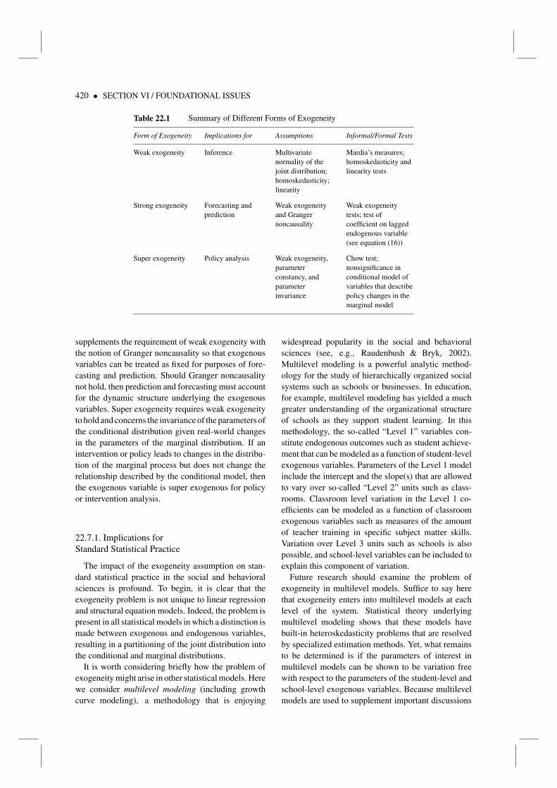
To summarize, each form of exogeneity relates toa particular use of a statistical model. Table 22.1reviews the different forms of exogeneity, their spe-cific requirements, and informal tests. To review, weakexogeneity relates to the use of a model for purposes ofinference. It concerns the extent to which the param-eters of the marginal distribution of the exogenousvariable can be ignored when focusing on the condi-tional distribution of the endogenous variable given theexogenous variable. Should weak exogeneity not hold,then estimation must account for both the marginaland conditional distributions. Strong exogeneity

420 • SECTION VI / FOUNDATIONAL ISSUES

Table 22.1 Summary of Different Forms of Exogeneity

Form of Exogeneity Implications for Assumptions Informal/Formal Tests

Weak exogeneity Inference Multivariatenormality of thejoint distribution;homoskedasticity;linearity

Mardia’s measures;homoskedasticity andlinearity tests

Strong exogeneity Forecasting andprediction

Weak exogeneityand Grangernoncausality

Weak exogeneitytests; test ofcoefficient on laggedendogenous variable(see equation (16))

Super exogeneity Policy analysis Weak exogeneity,parameterconstancy, andparameterinvariance

Chow test;nonsignificance inconditional model ofvariables that describepolicy changes in themarginal model

supplements the requirement of weak exogeneity withthe notion of Granger noncausality so that exogenousvariables can be treated as fixed for purposes of fore-casting and prediction. Should Granger noncausalitynot hold, then prediction and forecasting must accountfor the dynamic structure underlying the exogenousvariables. Super exogeneity requires weak exogeneityto hold and concerns the invariance of the parameters ofthe conditional distribution given real-world changesin the parameters of the marginal distribution. If anintervention or policy leads to changes in the distribu-tion of the marginal process but does not change therelationship described by the conditional model, thenthe exogenous variable is super exogenous for policyor intervention analysis.

22.7.1. Implications forStandard Statistical Practice

The impact of the exogeneity assumption on stan-dard statistical practice in the social and behavioralsciences is profound. To begin, it is clear that theexogeneity problem is not unique to linear regressionand structural equation models. Indeed, the problem ispresent in all statistical models in which a distinction ismade between exogenous and endogenous variables,resulting in a partitioning of the joint distribution intothe conditional and marginal distributions.

It is worth considering briefly how the problem ofexogeneity might arise in other statistical models. Herewe consider multilevel modeling (including growthcurve modeling), a methodology that is enjoying

widespread popularity in the social and behavioralsciences (see, e.g., Raudenbush & Bryk, 2002).Multilevel modeling is a powerful analytic method-ology for the study of hierarchically organized socialsystems such as schools or businesses. In education,for example, multilevel modeling has yielded a muchgreater understanding of the organizational structureof schools as they support student learning. In thismethodology, the so-called “Level 1” variables con-stitute endogenous outcomes such as student achieve-ment that can be modeled as a function of student-levelexogenous variables. Parameters of the Level 1 modelinclude the intercept and the slope(s) that are allowedto vary over so-called “Level 2” units such as class-rooms. Classroom level variation in the Level 1 co-efficients can be modeled as a function of classroomexogenous variables such as measures of the amountof teacher training in specific subject matter skills.Variation over Level 3 units such as schools is alsopossible, and school-level variables can be included toexplain this component of variation.

Future research should examine the problem ofexogeneity in multilevel models. Suffice to say herethat exogeneity enters into multilevel models at eachlevel of the system. Statistical theory underlyingmultilevel modeling shows that these models havebuilt-in heteroskedasticity problems that are resolvedby specialized estimation methods. Yet, what remainsto be determined is if the parameters of interest inmultilevel models can be shown to be variation freewith respect to the parameters of the student-level andschool-level exogenous variables. Because multilevelmodels are used to supplement important discussions

Chapter 22 / On Exogeneity • 421

of education policy, assessing the weak exogeneity ofpolicy-relevant variables is crucial.

A special case of multilevel modeling is growthcurve modeling, a methodology that is also enjoyingtremendous popularity in the social sciences anddirectly accounts for the dynamic features of paneldata. In such models, the Level 1 endogenous variableis an outcome such as a reading proficiency scorefor a particular student measured over multiple occa-sions. This score is modeled as a function of a timedimension such as grade level, as well as possiblytime-varying covariates such as parent involvement inreading activities. The parameters of the Level 1 modelconstitute the initial level and rate of change, and theseare allowed to vary randomly over individuals, whoare in turn modeled as a function of time-invariantexogenous variables such as race/ethnicity, gender, orperhaps experience in an early childhood interventionprogram. Variation in average initial level and rate ofchange can also be modeled as a function of Level 3units such as classrooms or schools. The power ofthis methodology is that it allows one to study indi-vidual and group contributions to individual growthover time.

The problem of exogeneity enters growth curvemodels in a variety of ways. First, repeated mea-sures on individuals can be a function of time-invariantvariables. For example, in estimating growth in read-ing proficiency in the younger grades, time-invariantvariables might include the IQ of the children (assumedto be stable over time), the income of the parents,and so on. Again, these variables are assumed to beexogenous.

Second, the repeated outcomes can be modeledas a function of time-varying covariates. Each time-varying covariate is presumed to be exogenous to itsrespective outcomes and is used to help explain, forexample, seasonal trends in the data. However, time-varying variables can also be allowed to have a laggedeffect on later outcomes. For example, a time-varyingcovariate such as parental reading activities at time tcan be specified to influence reading achievement attime t as well as reading achievement at time t + 1.This represents the introduction of a lagged exoge-nous variable into the full-growth curve model, andso issues of strong exogeneity and Granger noncausal-ity may be of relevance. In other words, the Level 1model that characterizes achievement at time t as afunction of time-varying covariates assumes that thetime-varying covariate at time t is not a function ofachievement at time t − 1. If this assumption does nothold, then the time-varying covariate is not stronglyexogenous.

In addition to the fact that exogeneity represents anissue in a wide range of statistical models, it must alsobe recognized that most statistical software packagesestimate the parameters of statistical models underthe untested assumption that weak exogeneity holds.In other words, software packages that engage inconditional estimation (e.g., conditional maximumlikelihood), conditional on the set of exogenousvariables, do so assuming that there is no informationin the marginal process that is relevant for the estima-tion of the conditional parameters. However, as notedabove, weak exogeneity is only valid if the joint distri-bution of the variables is multivariate normal—a heroicassumption at best. Therefore, it is likely in practicethat estimates derived under conditional estimation areincorrect. The only situation in which this is not aproblem is in estimation of the Gauss linear model withnonstochastic regressors. Future research and softwaredevelopment should explore methods of estimationthat account for the parameters of the marginal dis-tribution along with the conditional distribution for agiven specification of the form of the joint distributionof the data.

In the context of simple linear regression, infor-mal testing of weak exogeneity via assessing jointnormality and homoskedasticity is relatively straight-forward. Indeed, most standard statistical softwarepackages provide various direct and indirect tests ofthese assumptions. In the context of structural equationmodeling, however, although considerable attentionhas been paid to the normality assumption (see, e.g.,Kaplan, 2000, for a review), scant attention hasbeen paid to assessing assumptions of linearity andhomoskedasticity. This may be due to the fact that text-book treatments of structural equation modeling moti-vate the methodology from the viewpoint of the struc-tural form of the model, and therefore it is not directlyobvious how homoskedasticity could be assessed.However, if attention turns to the reduced form ofthe model as described in equation (8), then standardmethods for assessing the normality assumption—including homoskedasticity and linearity—would berelatively easy to implement. Therefore, users ofstructural equation modeling should be encouragedto study plots and other diagnostics associatedwith the multivariate linear model to assess weakexogeneity.

The issue raised here is not so much how toassess weak exogeneity but rather how to proceed ifthe assumption of weak exogeneity does not hold.Recognition of the seriousness of the exogeneityassumption should lead to fruitful research that focuseson estimation methods under alternative specifications

422 • SECTION VI / FOUNDATIONAL ISSUES

of the joint distribution of the data. In attemptingto characterize the joint distribution of the data, allmeans of data exploration should be encouraged. Thereshould be no concern about “finding a model in thedata” because the joint distribution of the data istheory free8 (Spanos, 1986). Theory information onlybecomes a problem when there is a factoring of thejoint distribution into the conditional and marginaldistributions insofar as that is the point in the mod-eling process, in which a substantive distinction ismade between endogenous and exogenous variablesand where parameters of interest are defined (seeSpanos, 1999).

The implications of the strong exogeneity assump-tion for statistical practice are relevant if models areused for prediction and forecasting. In this case, weakexogeneity is still a necessary requirement, but inaddition, it is imperative that Granger noncausalitybe established. Similarly, implications of the super-exogeneity assumption are relevant when models areused for policy or intervention evaluations. Superexogeneity also forces us to consider the require-ment of parameter constancy and invariance—issuesthat have not received as much attention in the socialand behavioral sciences as they should. Focusing onparameter constancy and invariance also forces usto consider whether there exist invariants in socialand behavioral processes. Moreover, as pointed outby Ericsson (1994), parameter constancy is a centralassumption of most estimation methods and hence isof vital importance to statistics generally.

22.7.2. Concluding Remarks

Our discussion throughout this chapter leads to therecognition that exogeneity is an adjective describingan assumed characteristic of a variable that is beingchosen for theoretical reasons to be an exogenousvariable. Weak exogeneity is the necessary condi-tion underlying all forms of exogeneity, and hencethis assumption is fundamental and requires empiri-cal confirmation to ensure valid inferences. Additionalassumptions are required to yield valid predictions orevaluations of policies or interventions.

Exogeneity resides at the nexus of the actual data-generating process (DGP) and the statistical modelused to understand that process. In the simplest

8. The exception being that theory enters into the choice of the variableset as well as methods of measurement. These issues are not trivial butare not central to our discussion of the role of theory as it pertains to theseparation of variables into endogenous and exogenous variables.

terms, the actual DGP is the real-life mechanism thatgenerated the observed data. It is the reference pointfor both the theory and the statistical model. In theformer case, the theory is put forth to explain thereality under investigation—for example, the organi-zational structure of schooling that generates studentachievement. In the latter case, the statistical modelis designed to capture the statistical features of thataspect of the actual DGP that we choose to study andmeasure (Spanos, 1986; see also Kaplan, 2000).

In addition to the role that exogeneity plays withregard to fundamental distinctions between theory,the DGP, and statistical models, exogeneity raises anumber of other important philosophical questions thatare central to the practice of statistical modeling in thesocial and behavioral sciences. One issue, for example,concerns the proper place of data mining as a premod-eling strategy. We find that when attention focuses oncharacterizing the joint distribution of the data, thendata mining has a central role to play. Another issuearising from our study of exogeneity concerns thedynamic reality of the phenomenon under investiga-tion. Granger noncausality and strong exogeneity forceus to consider exogenous variables as possibly beingresponsive to their own dynamic structure and thatthis must be correctly modeled to obtain accurate esti-mates for prediction and forecasting. Super exogeneityreminds us that our models are sensitive to real-lifechanges in the process under investigation. Finally,serious consideration of the problem of exogeneityforces us to reexamine statistical textbooks in the socialand behavioral sciences to clarify ambiguous conceptsand historical developments. It is hoped that reflectingon the importance of the exogeneity assumption willlead to a critical assessment of the methods of statisticalmodeling in the social and behavioral sciences.

References

Bollen, K. A. (1989). Structural equations with latent variables.New York: John Wiley.

Browne, M. W. (1984). Asymptotic distribution free methodsin the analysis of covariance structures. British Journal ofMathematical and Statistical Psychology, 37, 62–83.

Chow, G. C. (1960). Tests of equality between sets of coefficientsin two linear regressions. Econometrica, 28, 591–605.

Cohen, J., & Cohen, P. (1983). Applied multiple regression/correlation for the behavioral sciences. Mahwah, NJ:Lawrence Erlbaum.

Engle, R. F., & Hendry, D. F. (1993). Testing super exo-geneity and invariance in regression models. Journal ofEconometrics, 56, 119–139.

Chapter 22 / On Exogeneity • 423

Ericsson, N. R. (1994). Testing exogeneity: An introduction.In N. R. Ericsson & J. S. Irons (Eds.), Testing exogeneity(pp. 3–38). Oxford, UK: Oxford University Press.

Ericsson, N. R., & Irons, J. S. (Eds.). (1994). Testing exogeneity.Oxford, UK: Oxford University Press.

Fisher, F. (1966). The identification problem in econometrics.New York: McGraw-Hill.

Granger, C. W. J. (1969). Investigating causal relations byeconometric models and cross-spectral methods. Economet-rica, 37, 424–438.

Hendry, D. F. (1995). Dynamic econometrics. Oxford, UK:Oxford University Press.

Joreskog, K. G. (1973). A general method for estimating alinear structural equation system. In A. S. Goldberger &O. D. Duncan (Eds.), Structural equation models in the socialsciences (pp. 85–112). New York: Academic Press.

Kaplan, D. (2000). Structural equation modeling: Foundationsand extensions. Thousand Oaks, CA: Sage.

Kirk, R. E. (1995). Experimental design: Procedures for thebehavioral sciences. Pacific Grove, CA: Brooks/Cole.

Legendre, A. M. (1805). Nouvelles methods pour la determi-nation des orbites des cometes (New methods for determiningthe orbits of comets). Paris: Firmin Didot.

Lucas, R. E. (1976). Econometric policy evaluation: A critique.Journal of Monetary Economics, 1(Suppl.), 19–46.

Mardia, K. V. (1970). Measures of multivariate skewness andkurtosis with applications. Biometrika, 57, 519–530.

Mulaik, S. A. (1985). Exploratory statistics and empiricism.Philosophy of Science, 52, 410–430.

Muthen, B. (1984). A general structural equation model withdichotomous, ordered categorical, and continuous latentvariable indicators. Psychometrika, 49, 115–132.

Raudenbush, S. W., & Bryk, A. S. (2002). Hierarchical linearmodels: Applications and data analysis methods (2nd ed.).Thousands Oaks, CA: Sage.

Richard, J.-F. (1982). Exogeneity, causality, and structuralinvariance in econometric modeling. In G. C. Chow &P. Corsi (Eds.), Evaluating the reliability of macro-economicmodels (pp. 105–118). New York: John Wiley.

Spanos, A. (1986). Statistical foundations of econometricmodeling. Cambridge, UK: Cambridge University Press.

Spanos, A. (1999). Probability theory and statistical inference.Cambridge, UK: Cambridge University Press.

White, H. (1980). A heteroskedasticity-consistent covariancematrix estimator and a direct test for heteroskedasticity.Econometrica, 48, 817–838.

Wonnacott, R. J., & Wonnacott, T. H. (1979). Econometrics(2nd ed.). New York: John Wiley.

Yule, G. U. (1897). On the theory of correlation. Journal of theRoyal Statistical Society, 60, 812–854.