CHAPTER 22 POLARIMETRY - UGentphotonics.intec.ugent.be/education/IVPV/res_handbook/v2ch22.pdf ·...
37
CHAPTER 22 POLARIMETRY Russell A. Chipman Physics Department Uniy ersity of Alabama in Huntsy ille Huntsy ille , Alabama 22.1 GLOSSARY A analyzer vector a analyzer vector element a semimajor axis of ellipse BRDF bidirectional reflectance distribution function b semiminor axis of ellipse D diattenuation DOCP degree of circular polarization DOLP degree of linear polarization DOP degree of polarization Dep depolarization E extinction ratio e ellipticity I inhomogeneity of a Mueller matrix ID ideal depolarizer J Jones matrix j xx , j xy , j yx , j yy Jones matrix elements LD linear diattenuation LP linear polarizer M Mueller matrix M ¢ Mueller vector MBRDF Mueller bidirectional reflectance distribution function M D diattenuator Mueller matrix M R retarder Mueller matrix m 00 , m 01 , . . . , m 33 Mueller matrix elements Dn birefringence 22.1
Transcript of CHAPTER 22 POLARIMETRY - UGentphotonics.intec.ugent.be/education/IVPV/res_handbook/v2ch22.pdf ·...

CHAPTER 22 POLARIMETRY
Russell A . Chipman Physics Department Uni y ersity of Alabama in Hunts y ille Hunts y ille , Alabama
2 2 . 1 GLOSSARY
A analyzer vector a analyzer vector element a semimajor axis of ellipse
BRDF bidirectional reflectance distribution function b semiminor axis of ellipse D diattenuation
DOCP degree of circular polarization DOLP degree of linear polarization
DOP degree of polarization
Dep depolarization E extinction ratio e ellipticity
I inhomogeneity of a Mueller matrix
ID ideal depolarizer
J Jones matrix
j x x , j x y , j y x , j y y Jones matrix elements
LD linear diattenuation
LP linear polarizer
M Mueller matrix
M ¢ Mueller vector
MBRDF Mueller bidirectional reflectance distribution function
M D diattenuator Mueller matrix
M R retarder Mueller matrix
m 0 0 , m 0 1 , . . . , m 3 3 Mueller matrix elements
D n birefringence
22 .1
22 .2 OPTICAL INSTRUMENTS
n 1 , n 2 refractive indices of a birefringent medium
P flux measurement vector
P polarizance
P flux measurement
PD partial depolarizer
PDL polarization-dependent loss
QWLR quarter-wave linear retarder
Q index limit
q index for a sequence of polarization elements
R M rotational change of basis matrix for Stokes vectors
S Stokes vector
S ̂ normalized polarized Stokes vector
S 9 exiting Stokes vector
S m measured Stokes vector
S m a x , S m i n incident Stokes vectors of maximum and minimum intensity transmittance
s 0 , s 1 , s 2 , s 3 Stokes vector elements
T transpose , superscript
T intensity transmittance
T a v g intensity transmission averaged over all incident polarization states
T m a x maximum intensity transmittance
T m i n minimum intensity transmittance
Tr trace of a matrix
t thickness
U Jones / Mueller transformation matrix
VD variable partial depolarizer
W polarimetric measurement matrix
W 2 1 polarimetric data reduction matrix
W 2 1 P pseudoinverse of W
a , b angles of incidence
g , d angles of scatter
d retardance
h azimuth of ellipse
e eccentricity

POLARIMETRY 22 .3
θ orientation angle D θ angular increment
r amplitudes of a complex number f phases of a complex number
χ angle between the eigenpolarizations on the Poincare sphere ̂ tensor product
† Hermitian adjoint
2 2 . 2 OBJECTIVES
This chapter surveys the principles of polarization measurements . Throughout this chapter all measured and derived quantities are formulated in terms of the Stokes vector and Mueller matrix , as these comprise the most appropriate representation of polarization for radiometric measurements . The Mueller matrix has a structure which is dif ficult to understand , so the interpretation has been discussed within this chapter . One of the primary dif ficulties in performing accurate polarization measurements is the systematic errors due to nonideal polarization elements . Therefore , a formulation of the polarimetric measurement and data reduction process is included which readily handles arbitrary polarization elements used in the polarimeter whose transmitted or analyzed Stokes vectors are determined through calibration . Finally , a survey of the literature on applications studies utilizing polarimeters has been included .
This chapter is closely related to the following Handbook of Optics chapters : ‘‘Polarization’’ (Vol . I , Chap . 5) by J . M . Bennett , ‘‘Polarizers’’ by J . M . Bennett (Vol . II , Chap . 3) , and ‘‘Ellipsometry’’ by R . M . A . Azzam (Vol . II , Chap . 27) .
2 2 . 3 POLARIMETERS
Polarimeters are optical instruments used for determining the polarization properties of light beams and samples . Polarimetry , the science of measuring polarization , is most simply characterized as radiometry with polarization elements . To perform accurate polarimetry , all the issues necessary for careful and accurate radiometry must be considered , together with many additional polarization issues . In this chapter , our emphasis is strictly on those additional polarization issues which must be mastered to accurately determine polarization properties from polarimetric measurements . Typical applications of polarimeters include the following : remote sensing of the earth and astronomical bodies , calibration of polarization elements , measuring the thickness and refractive indices of thin films (ellipsometry) , spectroscopic studies of materials , and alignment of polarization-critical optical systems . We can broadly subdivide polarimeters into the several categories as discussed in succeeding sections .
2 2 . 4 LIGHT - MEASURING AND SAMPLE - MEASURING POLARIMETERS
Light-measuring polarimeters determine the polarization state of a beam of light or determine some of its polarization characteristics . These determinations may include the following : the direction of oscillation of the electric field vector for a linearly polarized

22 .4 OPTICAL INSTRUMENTS
beam , the helicity of a circularly polarized beam , or the elliptical parameters of an elliptically polarized beam , as well as the degree of polarization and other characteristics . A light-measuring polarimeter utilizes a set of polarization elements placed in a beam of light in front of a radiometer ; or , to paraphrase , the light from the sample is analyzed by a series of polarization state analyzers , and a set of measurements is acquired . The polarization characteristics of the sample are determined from these measurements by a data reduction procedure . Measurement , calibration , and data reduction algorithms are treated under ‘‘Light-measuring Polarimeters . ’’
2 2 . 5 SAMPLE - MEASURING POLARIMETERS
Sample-measuring polarimeters determine the relationship between the polarization states of incident and exiting beams for a sample . The term exiting beam is general and includes beams which are transmitted , reflected , dif fracted , or scattered . The term sample is also an inclusive term used in a broad sense to describe a general light-matter interaction or sequence of such interactions and applies to practically anything . Measurements are acquired using a series of polarization elements located between a source and sample and the exiting beams are analyzed with a separate set of polarization elements between the sample and radiometer . Samples of great interest include surfaces , thin films on surfaces , polarization elements , optical elements , optical systems , natural scenes , biological samples , and industrial samples .
Accurate polarimetric measurements can be made only if the polarization generator and / or polarization analyzer are fully calibrated . To perform accurate polarimetry , the polarization elements do not need to be ideal . If the Mueller matrices of the polarization components are known , the systematic errors due to nonideal polarization elements can be removed during the data reduction (see ‘‘Polarimetric Measurement Equation and Polarimetric Data Reduction Equation’’) .
2 2 . 6 COMPLETE AND INCOMPLETE POLARIMETERS
A light-measuring polarimeter is ‘‘complete’’ if it measures a Stokes vector or if a Stokes vector can be determined from its measurements . An ‘‘incomplete’’ light-measuring polarimeter cannot be used to determine a Stokes vector . For example , a polarimeter which employs a rotating polarizer in front of a detector does not determine the circular polarization content of a beam , and is incomplete . Similarly , a sample-measuring polarimeter is complete if it is capable of measuring the full Mueller matrix , and incomplete otherwise . Complete polarimeters are often referred to as Stokes polarimeters or Mueller polarimeters .
2 2 . 7 POLARIZATION GENERATORS AND ANALYZERS
A polarization generator consists of a source , optical elements , and polarization elements to produce a beam of known polarization state . A polarization generator is specified by the Stokes vector S of the exiting beam . A polarization analyzer is a configuration of polarization elements , optical elements , and a detector which performs a flux measure- ment of a particular polarization component in an incident beam . A polarization analyzer is characterized by a Stokes-like analyzer y ector A which specifies the incident
POLARIMETRY 22 .5
polarization state which is analyzed , the state which produces the maximal response at the detector . Sample-measuring polarimeters require polarization generators and polarization analyzers , while light-measuring polarimeters only require polarization analyzers . Fre- quently the terms ‘‘polarization generator’’ and ‘‘polarization analyzer’’ refer just to the polarization elements in the generator and analyzer . In this usage , it is important to distinguish between elliptical (and circular) generators and elliptical analyzers for a given state because they generally have dif ferent polarization characteristics and Mueller matrices (see ‘‘Elliptical and Circular Polarizers and Analyzers’’) .
2 2 . 8 CLASSES OF LIGHT - MEASURING POLARIMETERS
Polarimeters operate by acquiring measurements with a set of polarization analyzers (and a set of polarization generators for sample-measuring instruments) . The following sections classify polarimeters by the four broad methods by which these multiple measurements are acquired .
2 2 . 9 TIME - SEQUENTIAL MEASUREMENTS
In a time-sequential polarimeter , the measurements are taken sequentially in time . Between measurements , the polarization analyzer and / or polarization generator is changed . Time-sequential polarimeters frequently employ rotating polarization elements or filter wheels containing a set of analyzers . A time-sequential polarimeter generally employs a single source and detector .
2 2 . 1 0 POLARIZATION MODULATION
Polarimeters employing polarization modulation comprise a subset of time-sequential polarimeters . Here , the polarization analyzer contains a polarization modulator , a rapidly changing polarization element . The output of the analyzer is a rapidly fluctuating irradiance on which polarization information is encoded . Polarization parameters can then be determined by ac and vector voltmeters , by lock-in amplifiers , or by frequency-domain digital signal processing techniques . For example , a rapidly spinning polarizer produces a modulated output which allows the flux and the degree of linear polarization to be read with a dc voltmeter and an ac voltmeter . The most common high-speed polarization modulators in general use are the electro-optical modulator , the magneto-optical modula- tor , and the photoelastic modulator .
2 2 . 1 1 DIVISION OF APERTURE
Polarimeters based on division of aperture employ multiple polarization analyzers operating side-by-side . The aperture of the polarimeter is subdivided , with each beam going into a separate polarization analyzer and detector . The detectors are usually

22 .6 OPTICAL INSTRUMENTS
synchronized to acquire measurements simultaneously . This is similar in principle to the polarizing glasses used in 3-D movie systems , where a 45 8 polarizer is used for one eye and a 135 8 for the other , permitting two polarization measurements simultaneously in two eyes .
2 2 . 1 2 DIVISION OF AMPLITUDE
Division-of-amplitude polarimeters utilize beam splitters to divide beams and direct them toward multiple analyzers and detectors . A division-of-amplitude polarimeter can acquire its measurements simultaneously . Many division-of-amplitude polarimeters use polarizing beam splitters to simultaneously divide and analyze the polarization state of the beam . The four-detector photopolarimeter uses a sequence of detectors at nonormal incidence to measure Stokes vectors (Azzam , 1985 ; Azzam , Elminyawi , and El-Saba , 1988) .
2 2 . 1 3 DEFINITIONS
Analyzer —an element whose intensity transmission is proportional to the content of a specific polarization state in the incident beam . Analyzers are placed before the detector in polarimeters . The transmitted polarization state emerging from an analyzer is not necessarily the same as the state which is being analyzed .
Birefringence —a material property , the retardance associated with propagation through an anisotropic medium . For each propagation direction within a birefringent medium , there are two modes of propagation with dif ferent refractive indices n 1 and n 2 . The birefringence D n is D n 5 u n 1 2 n 2 u .
Depolarization —a process which couples polarized light into unpolarized light . Depolarization is intrinsically associated with scattering and with diattenuation and retardance which vary in space , time , and / or wavelength .
Diattenuation —the property of an optical element or system whereby the intensity transmittance of the exiting beam depends on the polarization state of the incident beam . The intensity transmittance is a maximum P m a x for one incident state , and a minimum P m i n for the orthogonal state . The diattenuation is defined as ( P m a x 2 P m i n ) / ( P m a x 1 P m i n ) .
Diattenuator —any homogeneous polarization element which displays significant diattenuation and minimal retardance . Polarizers have a diattenuation close to one , but nearly all optical interfaces are weak diattenuators . Examples of diattenuators include the following : polarizers and dichroic materials , as well as metal and dielectric interfaces with reflection and transmission dif ferences described by Fresnel equations ; thin films (homogeneous and isotropic) ; and dif fraction gratings .
Dichroism —the material property of displaying diattenuation during propagation . For each direction of propagation , dichroic media have two modes of propagation with dif ferent absorption coef ficients . Examples of dichroic materials include sheet polarizers and dichroic crystals such as tourmaline .
Eigenpolarization —a polarization state transmitted unaltered by a polarization element except for a change of amplitude and phase . Every polarization element has two

POLARIMETRY 22 .7
eigenpolarizations . Any incident light not in an eigenpolarization state is transmitted in a polarization state dif ferent from the incident state . Eigenpolarizations are the eigenvectors of the corresponding Mueller or Jones matrix . Ellipsometry —a polarimetric technique which uses the change in the state of polariza- tion of light upon reflection for the characterization of surfaces , interfaces , and thin films (after Azzam , 1993) . Homogeneous polarization element —an element whose eigenpolarizations are orthogo- nal . Then , the eigenpolarizations are the states of maximum and minimum transmit- tance and also of maximum and minimum optical path length . A homogeneous element is classified as linear , circular , or elliptical depending on the form of the eigenpolarizations . Inhomogeneous polarization element —an element whose eigenpolarizations are not orthogonal . Such an element will display dif ferent polarization characteristics for forward and backward propagating beams . The eigenpolarizations are generally not the states of maximum and minimum transmittance . Often inhomogeneous elements cannot be simply classified as linear , circular , or elliptical . Ideal polarizer —a polarizer with an intensity transmittance of one for its principal state and an intensity transmittance of zero for the orthogonal state . Linear polarizer —a device which , when placed in an incident unpolarized beam , produces a beam of light whose electric field vector is oscillating primarily in one plane , with only a small component in the perpendicular plane (after Bennett , 1993) . Nonpolarizing element —an element which does not change the polarization state for arbitrary states . The polarization state of the output light is equal to the polarization state of the incident light for all possible input polarization states . Partially polarized light —light containing an unpolarized component ; cannot be extinguished by an ideal polarizer . Polarimeter —an optical instrument for the determination of the polarization state of a light beam , or the polarization-altering properties of a sample . Polarimetry —the science of measuring the polarization state of a light beam and the diattenuating , retarding , and depolarizing properties of materials . Polarization —any process which alters the polarization state of a beam of light , including diattenuation , retardance , depolarization , and scattering . Polarization coupling —any conversion of light from one polarization state into another state . Polarized light —light in a fixed , elliptically (including linearly or circularly) polarized state . It can be extinguished by an ideal polarizer . For polychromatic light , the polarization ellipses associated with each spectral component have identical ellipticity , orientation , and helicity . Polarizer —a strongly diattenuating optical element designed to transmit light in a specified polarization state independent of the incident polarization state . The transmission of one of the eigenpolarizations is very nearly zero . Polarization element —any optical element which alters the polarization state of light . This includes polarizers , retarders , mirrors , thin films , and nearly all optical elements . Pure diattenuator —a diattenuator with zero retardance and no depolarization . Pure retarder —a retarder with zero diattenuation and no depolarization . Retardance —a polarization-dependent phase change associated with a polarization element or system . The phase (optical path length) of the output beam depends upon the polarization state of the input beam . The transmitted phase is a maximum for one
22 .8 OPTICAL INSTRUMENTS
eigenpolarization , and a minimum for the other eigenpolarization . Other states show polarization coupling and an intermediate phase . Retardation plate —a retarder constructed from a plane parallel plate or plates of linearly birefringent material . Retarder —a polarization element designed to produce a specified phase dif ference between the exiting beams for two orthogonal incident polarization states (the eigenpolarizations of the element) . For example , a quarter-wave linear retarder has as its eigenpolarizations two orthogonal linearly polarized states which are transmitted in their incident polarization states but with a 90 8 (quarter-wavelength) relative phase dif ference introduced . Spectropolarimetry —the spectroscopic study of the polarization properties of materials . Spectropolarimetry is a generalization of conventional optical spectroscopy . Where conventional spectroscopy endeavors to measure the reflectance or transmission of a sample as a function of wavelength , spectropolarimetry also determines the diattenuat- ing , retarding , and depolarizing properties of the sample . Complete characterization of these properties is accomplished by measuring the Mueller matrix of the sample as a function of wavelength . Wa y eplate —a retarder .
2 2 . 1 4 STOKES VECTORS AND MUELLER MATRICES
Several calculi have been developed for analyzing polarization , including those based on the Jones matrix , coherency matrix , Mueller matrix , and other matrices (Shurclif f , 1962 ; Gerrard and Burch , 1975 ; Theocaris and Gdoutos , 1979 ; Azzam and Bashara , 1987 ; Coulson , 1988 ; Egan , 1992) . Of these methods , the Mueller calculus is most generally suited for describing irradiance-measuring instruments , including most polarimeters , radiometers , and spectrometers , and is used exclusively in this paper .
In the Mueller calculus , the Stokes vector S is used to describe the polarization state of a light beam , and the Mueller matrix M to describe the polarization-altering characteristics of a sample . This sample may be a surface , a polarization element , an optical system , or some other light / matter interaction which produces a reflected , refracted , dif fracted , or scattered light beam . All vectors and matrices are represented by bold characters . Normalized vectors have ‘‘hats’’ (i . e ., A ̂ ) .
2 2 . 1 5 PHENOMENOLOGICAL DEFINITION OF THE STOKES VECTOR
The Stokes vector is defined relative to the following six flux measurements P performed with ideal polarizers in front of a radiometer (Shurclif f , 1962) :
P H horizontal linear polarizer (0 8 )
P V vertical linear polarizer (90 8 )
P 4 5 45 8 linear polarizer
P 1 3 5 135 8 linear polarizer
P R right circular polarizer
P L left circular polarizer

POLARIMETRY 22 .9
Normally , these measurements are irradiance measurements ( W / m 2 ) although other flux measurements might be used . The Stokes vector is defined as
S 5 3 s 0
s 1
s 2
s 3
4 5 3 P H 1 P V
P H 2 P V
P 4 5 2 P 1 3 5
P R 2 P L
4 (1)
where s 0 , s 1 , s 2 , and s 3 are the Stokes vector elements . The Stokes vector does not need to be measured by these six ideal measurements ; what is required is that other methods reproduce the Stokes vector defined in this manner . Ideal polarizers are not required . Further , the Stokes vector is a function of wavelength , position on the object , and the light’s direction of emission or scatter . Thus , a Stokes vector measurement is an average over area , solid angle , and wavelength , as is any radiometric measurement . Each Stokes vector element has units of watts per meter squared . The Stokes vector is defined relative to a local x 2 y coordinate system defined in the plane perpendicular to the propagation vector . The coordinate system is right-handed ; the cross product x ̂ 3 y ̂ of the basis vectors points in the direction of propagation of the beam .
2 2 . 1 6 POLARIZATION PROPERTIES OF LIGHT BEAMS
From the Stokes vector , the following polarization parameters are determined (Azzam and Bashara , 1977 and 1987 ; Kliger , Lewis , and Randall , 1990 ; Collett , 1992) : Flux P 5 s 0 (2)
Degree of polarization DOP 5 4 s 2
1 1 s 2 2 1 s 2
3
s 0 (3)
Degree of linear polarization DOLP 5 4 s 2
1 1 s 2 2
s 0 (4)
Degree of circular polarization DOCP 5 s 3
s 0 (5)
The Stokes vector for a partially polarized beam ( DOP , 1) can be considered as a superposition of a completely polarized Stokes vector S P and an unpolarized Stokes vector S U which are uniquely related to S as follows (Collett , 1992) :
S 5 S P 1 S U 5 3 s 0
s 1
s 2
s 3
4 5 s 0 DOP 3 1
s 1 / ( s 0 DOP ) s 2 / ( s 0 DOP ) s 3 / ( s 0 DOP )
4 1 (1 2 DOP ) s 0 3 1 0 0 0 4 (6)
The polarized portion of the beam represents a net polarization ellipse traced by the electric field vector as a function of time . The ellipse has a magnitude of the semimajor axis a , semiminor axis b , orientation of the major axis h (azimuth of the ellipse) measured counterclockwise from the x axis , and eccentricity (or ellipticity) .
Ellipticity e 5 b a
5 s 3
s 0 1 4 s 2 1 1 s 2
2 (7)
Orientation of major axis , azimuth h 5 1 – 2 arctan F s 2
s 1 G (8)
Eccentricity e 5 4 1 2 e 2 (9)
The ellipticity is the ratio of the minor to the major axis of the corresponding electric field
22 .10 OPTICAL INSTRUMENTS
polarization ellipse , and varies from 0 for linearly polarized light to 1 for circularly polarized light . The polarization ellipse is alternatively described by its eccentricity , which is zero for circularly polarized light , increases as the ellipse becomes thinner (more cigar-shaped) , and becomes one for linearly polarized light .
2 2 . 1 7 MUELLER MATRICES
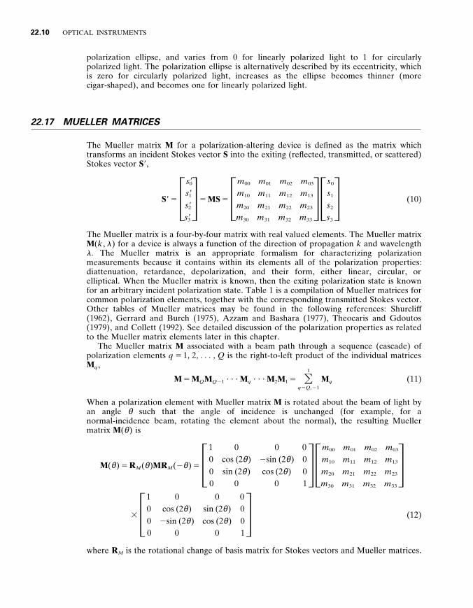
The Mueller matrix M for a polarization-altering device is defined as the matrix which transforms an incident Stokes vector S into the exiting (reflected , transmitted , or scattered) Stokes vector S 9 ,
S 9 5 3 s 9 0
s 9 1
s 9 2
s 9 3 4 5 MS 5 3
m 0 0 m 0 1 m 0 2 m 0 3
m 1 0 m 1 1 m 1 2 m 1 3
m 2 0 m 2 1 m 2 2 m 2 3
m 3 0 m 3 1 m 3 2 m 3 3
4 3 s 0
s 1
s 2
s 3
4 (10)
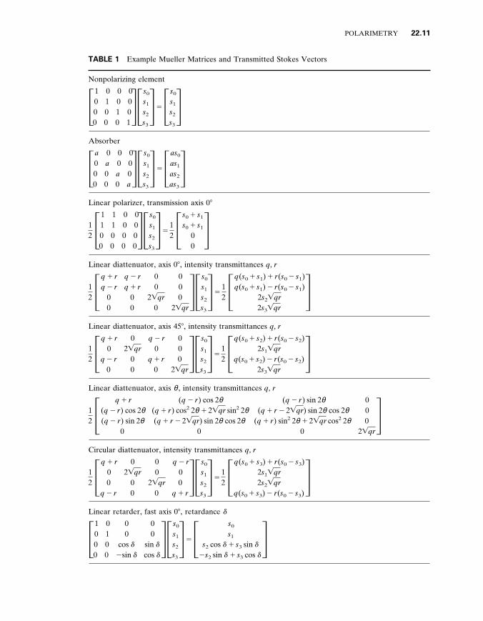
The Mueller matrix is a four-by-four matrix with real valued elements . The Mueller matrix M ( k , l ) for a device is always a function of the direction of propagation k and wavelength l . The Mueller matrix is an appropriate formalism for characterizing polarization measurements because it contains within its elements all of the polarization properties : diattenuation , retardance , depolarization , and their form , either linear , circular , or elliptical . When the Mueller matrix is known , then the exiting polarization state is known for an arbitrary incident polarization state . Table 1 is a compilation of Mueller matrices for common polarization elements , together with the corresponding transmitted Stokes vector . Other tables of Mueller matrices may be found in the following references : Shurclif f (1962) , Gerrard and Burch (1975) , Azzam and Bashara (1977) , Theocaris and Gdoutos (1979) , and Collett (1992) . See detailed discussion of the polarization properties as related to the Mueller matrix elements later in this chapter .
The Mueller matrix M associated with a beam path through a sequence (cascade) of polarization elements q 5 1 , 2 , . . . , Q is the right-to-left product of the individual matrices M q ,
M 5 M Q M Q 2 1 ? ? ? M q ? ? ? M 2 M 1 5 O 1
q 5 Q , 2 1 M q (11)
When a polarization element with Mueller matrix M is rotated about the beam of light by an angle θ such that the angle of incidence is unchanged (for example , for a normal-incidence beam , rotating the element about the normal) , the resulting Mueller matrix M ( θ ) is
M ( θ ) 5 R M ( θ ) MR M ( 2 θ ) 5 3 1 0 0 0
0 cos (2 θ ) sin (2 θ )
0
0 2 sin (2 θ ) cos (2 θ )
0
0 0 0 1 4 3
m 0 0 m 0 1 m 0 2 m 0 3
m 1 0 m 1 1 m 1 2 m 1 3
m 2 0 m 2 1 m 2 2 m 2 3
m 3 0 m 3 1 m 3 2 m 3 3
4 3 3
1 0 0 0
0 cos (2 θ )
2 sin (2 θ ) 0
0 sin (2 θ ) cos (2 θ )
0
0 0 0 1 4 (12)
where R M is the rotational change of basis matrix for Stokes vectors and Mueller matrices .
POLARIMETRY 22 .11
TABLE 1 Example Mueller Matrices and Transmitted Stokes Vectors
Nonpolarizing element
3 1 0 0 0 0 1 0 0 0 0 1 0 0 0 0 1
4 3 s 0
s 1
s 2
s 3
4 5 3 s 0
s 1
s 2
s 3
4 Absorber
3 a 0 0 0 0 a 0 0 0 0 a 0 0 0 0 a
4 3 s 0
s 1
s 2
s 3
4 5 3 as 0
as 1
as 2
as 3
4 Linear polarizer , transmission axis 0 8
1 2 3
1 1 0 0 1 1 0 0 0 0 0 0 0 0 0 0
4 3 s 0
s 1
s 2
s 3
4 5 1 2 3
s 0 1 s 1
s 0 1 s 1
0 0
4 Linear diattenuator , axis 0 8 , intensity transmittances q , r
1 2 3
q 1 r q 2 r
0 0
q 2 r q 1 r
0 0
0 0
2 4 qr 0
0 0 0
2 4 qr 4 3
s 0
s 1
s 2
s 3
4 5 1 2 3
q ( s 0 1 s 1 ) 1 r ( s 0 2 s 1 ) q ( s 0 1 s 1 ) 2 r ( s 0 2 s 1 )
2 s 2 4 qr 2 s 3 4 qr
4 Linear diattenuator , axis 45 8 , intensity transmittances q , r
1 2 3
q 1 r 0
q 2 r 0
0 2 4 qr
0 0
q 2 r 0
q 1 r 0
0 0 0
2 4 qr 4 3
s 0
s 1
s 2
s 3
4 5 1 2 3
q ( s 0 1 s 2 ) 1 r ( s 0 2 s 2 ) 2 s 1 4 qr
q ( s 0 1 s 2 ) 2 r ( s 0 2 s 2 ) 2 s 3 4 qr
4 Linear diattenuator , axis θ , intensity transmittances q , r
1 2 3
q 1 r ( q 2 r ) cos 2 θ ( q 2 r ) sin 2 θ
0
( q 2 r ) cos 2 θ ( q 1 r ) cos 2 2 θ 1 2 4 qr sin 2 2 θ ( q 1 r 2 2 4 qr ) sin 2 θ cos 2 θ
0
( q 2 r ) sin 2 θ ( q 1 r 2 2 4 qr ) sin 2 θ cos 2 θ
( q 1 r ) sin 2 2 θ 1 2 4 qr cos 2 2 θ 0
0 0 0
2 4 qr 4
Circular diattenuator , intensity transmittances q , r
1 2 3
q 1 r 0 0
q 2 r
0 2 4 qr
0 0
0 0
2 4 qr 0
q 2 r 0 0
q 1 r 4 3
s 0
s 1
s 2
s 3
4 5 1 2 3
q ( s 0 1 s 3 ) 1 r ( s 0 2 s 3 ) 2 s 1 4 qr 2 s 2 4 qr
q ( s 0 1 s 3 ) 2 r ( s 0 2 s 3 ) 4
Linear retarder , fast axis 0 8 , retardance d
3 1 0 0 1 0 0 0 0
0 0
cos d
2 sin d
0 0
sin d
cos d 4 3
s 0
s 1
s 2
s 3
4 5 3 s 0
s 1
s 2 cos d 1 s 3 sin d
2 s 2 sin d 1 s 3 cos d 4

22 .12 OPTICAL INSTRUMENTS
TABLE 1 ( Continued )
Linear retarder , fast axis 45 8 , retardance d
3 1 0 0 0
0 cos d
0 sin d
0 0 1 0
0 2 sin d
0 cos d
4 3 s 0
s 1
s 2
s 3
4 5 3 s 0
s 1 cos d 2 s 3 sin d
s 2
s 1 sin d 1 s 3 cos d 4
Linear retarder , fast axis θ , retardance d
3 1 0 0 0
0 cos 2 2 θ 1 sin 2 2 θ cos d
sin 2 θ cos 2 θ (1 2 cos d ) sin 2 θ sin d
0 sin 2 θ cos 2 θ (1 2 cos d ) sin 2 2 θ 1 cos 2 2 θ cos d
2 cos 2 θ sin d
0 2 sin 2 θ sin d
cos 2 θ sin d
cos d 4
Circular retarder , retardance d
3 1 0 0 0
0 cos d
2 sin d
0
0 sin d
cos d
0
0 0 0 1 4 3
s 0
s 1
s 2
s 3
4 5 3 s 0
s 1 cos d 1 s 2 sin d
2 s 1 sin d 1 s 2 cos d
s 3 4
Linear diattenuator and retarder , fast axis 0 8 , intensity transmittance ( q , r ) , retardance d
1 2 3
q 1 r q 2 r
0 0
q 2 r q 1 r
0 0
0 0
2 4 qr cos d
2 2 4 qr sin d
0 0
2 4 qr sin d
2 4 qr cos d 4 3
s 0
s 1
s 2
s 3
4 5 1 2 3
q ( s 0 1 s 1 ) 1 r ( s 0 2 s 1 ) q ( s 0 1 s 1 ) 2 r ( s 0 2 s 1 )
2 4 qr ( s 2 cos d 1 s 3 sin d ) 2 4 qr ( 2 s 2 sin d 1 s 3 cos d )
4 Ideal depolarizer
3 1 0 0 0 0 0 0 0 0 0 0 0 0 0 0 0
4 3 s 0
s 1
s 2
s 3
4 5 3 s 0
0 0 0 4
Partial depolarizer
3 1 0 0 0 0 d 0 0 0 0 d 0 0 0 0 d
4 3 s 0
s 1
s 2
s 3
4 5 3 s 0
ds 1
ds 2
ds 3
4 Here θ . 0 if the x axis of the device is rotated toward 45 8 . If the polarization element remains fixed but the coordinate system rotates by f , the resulting Mueller matrix is M ( f ) 5 R M ( 2 f ) MR m ( f ) .
2 2 . 1 8 COORDINATE SYSTEM FOR THE MUELLER MATRIX
Consider a Mueller polarimeter consisting of a polarization generator which illuminates a sample , and a polarization analyzer which collects the light exiting the sample in a particular direction . We wish to characterize the polarization modification properties of the sample for a particular incident and exiting beam through the Mueller matrix . The
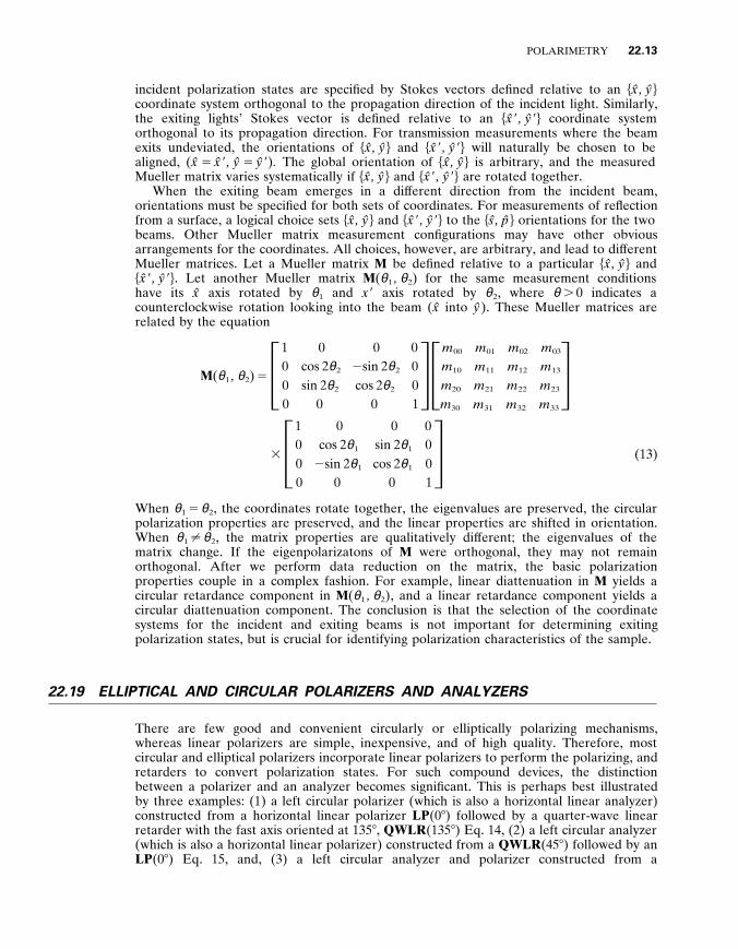
POLARIMETRY 22 .13
incident polarization states are specified by Stokes vectors defined relative to an h x ̂ , y ̂ j coordinate system orthogonal to the propagation direction of the incident light . Similarly , the exiting lights’ Stokes vector is defined relative to an h x ̂ 9 , y ̂ 9 j coordinate system orthogonal to its propagation direction . For transmission measurements where the beam exits undeviated , the orientations of h x ̂ , y ̂ j and h x ̂ 9 , y ̂ 9 j will naturally be chosen to be aligned , ( x ̂ 5 x ̂ 9 , y ̂ 5 y ̂ 9 ) . The global orientation of h x ̂ , y ̂ j is arbitrary , and the measured Mueller matrix varies systematically if h x ̂ , y ̂ j and h x ̂ 9 , y ̂ 9 j are rotated together .
When the exiting beam emerges in a dif ferent direction from the incident beam , orientations must be specified for both sets of coordinates . For measurements of reflection from a surface , a logical choice sets h x ̂ , y ̂ j and h x ̂ 9 , y ̂ 9 j to the h s ̂ , p ̂ j orientations for the two beams . Other Mueller matrix measurement configurations may have other obvious arrangements for the coordinates . All choices , however , are arbitrary , and lead to dif ferent Mueller matrices . Let a Mueller matrix M be defined relative to a particular h x ̂ , y ̂ j and h x ̂ 9 , y ̂ 9 j . Let another Mueller matrix M ( θ 1 , θ 2 ) for the same measurement conditions have its x ̂ axis rotated by θ 1 and x 9 axis rotated by θ 2 , where θ . 0 indicates a counterclockwise rotation looking into the beam ( x ̂ into y ̂ ) . These Mueller matrices are related by the equation
M ( θ 1 , θ 2 ) 5 3 1 0 0 0
0 cos 2 θ 2
sin 2 θ 2
0
0 2 sin 2 θ 2
cos 2 θ 2
0
0 0 0 1 4 3
m 0 0 m 0 1 m 0 2 m 0 3
m 1 0 m 1 1 m 1 2 m 1 3
m 2 0 m 2 1 m 2 2 m 2 3
m 3 0 m 3 1 m 3 2 m 3 3
4 3 3
1 0 0 0
0 cos 2 θ 1
2 sin 2 θ 1
0
0 sin 2 θ 1
cos 2 θ 1
0
0 0 0 1 4 (13)
When θ 1 5 θ 2 , the coordinates rotate together , the eigenvalues are preserved , the circular polarization properties are preserved , and the linear properties are shifted in orientation . When θ 1 ? θ 2 , the matrix properties are qualitatively dif ferent ; the eigenvalues of the matrix change . If the eigenpolarizatons of M were orthogonal , they may not remain orthogonal . After we perform data reduction on the matrix , the basic polarization properties couple in a complex fashion . For example , linear diattenuation in M yields a circular retardance component in M ( θ 1 , θ 2 ) , and a linear retardance component yields a circular diattenuation component . The conclusion is that the selection of the coordinate systems for the incident and exiting beams is not important for determining exiting polarization states , but is crucial for identifying polarization characteristics of the sample .
2 2 . 1 9 ELLIPTICAL AND CIRCULAR POLARIZERS AND ANALYZERS
There are few good and convenient circularly or elliptically polarizing mechanisms , whereas linear polarizers are simple , inexpensive , and of high quality . Therefore , most circular and elliptical polarizers incorporate linear polarizers to perform the polarizing , and retarders to convert polarization states . For such compound devices , the distinction between a polarizer and an analyzer becomes significant . This is perhaps best illustrated by three examples : (1) a left circular polarizer (which is also a horizontal linear analyzer) constructed from a horizontal linear polarizer LP (0 8 ) followed by a quarter-wave linear retarder with the fast axis oriented at 135 8 , QWLR (135 8 ) Eq . 14 , (2) a left circular analyzer (which is also a horizontal linear polarizer) constructed from a QWLR (45 8 ) followed by an LP (0 8 ) Eq . 15 , and , (3) a left circular analyzer and polarizer constructed from a

22 .14 OPTICAL INSTRUMENTS
QWLR (135 8 ) , then an LP (0 8 ) , followed by a QWLR (45 8 ) Eq . 16 . The Mueller matrix equations and exiting polarization states for arbitrary incident states are as follows :
QWLR (135 8 ) LP (0 8 ) S 5 1 2 3
1 1 0 0 0 0 0 0 0 0 0 0
2 1 2 1 0 0 4 3
s 0
s 1
s 2
s 3
4 5 1 2 3
s 0 1 s 1
0 0
2 s 0 2 s 1
4 (14)
LP (0 8 ) QWLR (45 8 ) S 5 1 2 3
1 0 0 2 1 1 0 0 2 1 0 0 0 0 0 0 0 0
4 3 s 0
s 1
s 2
s 3
4 5 1 2 3
s 0 2 s 3
s 0 2 s 3
0 0 4 (15)
QWLR (135 8 ) LP (0 8 ) QWLR (45 8 ) S 5 1 2 3
1 0 0 2 1 0 0 0 0 0 0 0 0
2 1 0 0 1 4 3
s 0
s 1
s 2
s 3
4 5 1 2 3
s 0 2 s 3
0 0
2 s 0 1 s 3
4 (16)
The device in Eq . (14) transmits only left circularly polarized light , because the zeroth and third elements have equal magnitude and opposite sign , making it a left circular polarizer . However , the transmitted flux ( s 0 1 s 1 ) / 2 is the flux of horizontal linearly polarized light in the incident beam , making it a horizontal linear analyzer . Similarly , the transmitted flux from the example in Eq . (15) , ( s 0 2 s 3 ) / 2 , is the flux of left circularly polarized light in the incident beam , making this combination a left circular analyzer . The final polarizer makes the device in Eq . (15) a horizontal linear polarizer , although this is not the standard Mueller matrix for horizontal linear polarizers found in tables . Thus an analyzer for a state does not necessarily transmit the state ; its transmitted flux is proportional to the amount of the analyzed state in the incident beam . Examples in Eqs . (14) and (15) are referred to as inhomogeneous polarization elements because the eigenpolarizations are not orthogo- nal , and the characteristics of the device are dif ferent for propagation in opposite directions . The device in Eq . (16) is both a left circular polarizer and a left circular analyzer ; it has the same characteristics for propagation in opposite directions , and is referred to as a homogeneous left circular polarizer .
2 2 . 2 0 LIGHT - MEASURING POLARIMETERS
This section presents a general formulation of the measurement and data reduction procedure for a polarimeter intended to measure the state of polarization of a light beam . Similar developments are found in Theil (1976) , Azzam (1990) , and Stenflo (1991) . A survey of light-measuring polarimeter configurations is found in the Handbook , Chap . 27 , ‘‘Ellipsometry’’ (Azzam , 1994) .
Stokes vectors and related polarization parameters for a beam are determined by measuring the flux transmitted through a set of polarization analyzers . Each analyzer determines the flux of one polarization component in the incident beam . Since a polarization analyzer does not contain ideal polarization elements , the analyzer must be calibrated , and the calibration data used in the data reduction . This section describes data reduction algorithms for determining Stokes vectors which assume arbitrary analyzers ; the algorithms allow for general calibration data to be used . Each analyzer is used to measure

POLARIMETRY 22 .15
one polarization component of the incident light . The measured values are related to the incident Stokes vector and the analyzers by the polarimetric measurement equation . A set of linear equations , the data reduction equations , is then solved to determine the Stokes parameters for the beam .
Henceforth , the ‘‘polarization analyzer’’ is considered as the polarization elements used for analyzing the polarization state together with any and all optical elements (lenses , mirrors , etc . ) , and the detector contained in the polarimeter . The polarization ef fects from all elements are included in the measurement and data reduction procedures for the polarimeter . A polarization analyzer is characterized by an analyzer y ector containing four elements and is defined in a manner analogous to a Stokes vector . Let P H be flux measurement taken by the detector (the current or voltage generated) when one unit of horizontally polarized light is incident . Similarly P V , P 4 5 , P 1 3 5 , P R , and P L are the detector’s flux measurements for the corresponding incident polarized beams with unit flux . Then the analyzer vector A is
A 5 3 a 0
a 1
a 2
a 3
4 5 3 P H 1 P V
P H 2 P V
P 4 5 2 P 1 3 5
P R 2 P L
4 (17)
Note that P H 1 P V 5 P 4 5 1 P 1 3 5 5 P R 1 P L . The response P of the polarization analyzer to an arbitrary polarization state S is the dot product
P 5 A ? S 5 a 0 s 0 1 a 1 s 1 1 a 2 s 2 1 a 3 s 3 (18)
A Stokes vector measurement consists of series of measurements taken with a set of polarization analyzers . Let the total number of analyzers be Q , with each analyzer A q specified by index q 5 0 , 1 , . . . , Q 2 1 . We assume the incident Stokes vector is the same for all polarization analyzers and strive to ensure this in our experimental setup . The q th measurement generates an output P q 5 A q ? S . A polarimetric measurement matrix W is defined as a four-by- Q matrix with the q th row containing the analyzer vector A q ,
W 5 3 a 0 , 0
a 1 , 0
? ? ? a Q 2 1 , 0
a 0 , 1
a 1 , 1
a Q 2 1 , 1
a 0 , 2
a 1 , 2
a Q 2 1 , 2
a 0 , 3
a 1 , 3
a Q 2 1 , 3
4 (19)
The Q measured flux values are arranged in a measurement vector P 5 [ P 0 , P 1 , . . . , P Q 2 1 ]
T ? P is related to S by the polarimetric measurement equation
P 5 3 P 0
P 1
? ? ? P Q 2 1
4 5 WS 5 3 a 0 , 0
a 1 , 0
? ? ? a Q 2 1 , 0
a 0 , 1
a 1 , 1
a Q 2 1 , 1
a 0 , 2
a 1 , 2
a Q 2 1 , 2
a 0 , 3
a 1 , 3
a Q 2 1 , 3
4 3 s 0
s 1
s 2
s 3
4 (20)
If W is accurately known , then this equation can be inverted to solve for the incident Stokes vector . During calibration of the polarimeter , the principal objective is the determination of the matrix W or equivalent information regarding the states which the polarimeter analyzes at each of its analyzer settings . However , systematic errors , dif ferences between the calibrated and actual W , will always be present .
To calculate the incident Stokes vector from the data , the inverse of W is determined and applied to the measured data . The measured value for the incident Stokes vector is designated S m to distinguish it from the actual S . In principle , S m is related to the data by the polarimetric data reduction matrix W 2 1 ,
S m 5 W 2 1 P (21)
22 .16 OPTICAL INSTRUMENTS
Three considerations in the solution of this equation are the existence , rank , and uniqueness of the matrix inverse W 2 1 .
The simplest case occurs when four measurements are performed . If Q 5 4 linearly independent measurements are made , W is of rank four , and the polarimetric measure- ment matrix W is nonsingular . Then W 2 1 exists and is unique . Data reduction is performed by Eq . 20 and the polarimeter measures all four elements of the incident Stokes vector .
The second case occurs when Q . 4 . With more than four measurements , W is not square , W 2 1 is not unique , and S m is overdetermined by the measurements . In the absence of noise in the measurements , the dif ferent W 2 1 would all yield the same value for S m . Because noise is always present , the optimum W 2 1 is desired . The least squares estimate for S m utilizes the psuedoinverse W 2 1
P of W , W 2 1 P 5 ( W T W ) 2 1 W T . The best estimate of S in
the presence of random noise is
S m 5 ( W T W ) 2 1 W T P (22)
The third case occurs when W is of rank three or less . The optimal matrix inverse is the pseudoinverse . However , only three or less of the Stokes vector elements can be determined from the data . The polarimeter is referred to as ‘‘incomplete . ’’ Figure 11 in Chap . 27 , ‘‘Ellipsometry , ’’ in this Handbook , summarizes polarization element configura- tions for Stokes vector measurements listing the vector elements not determined by the incomplete configurations .
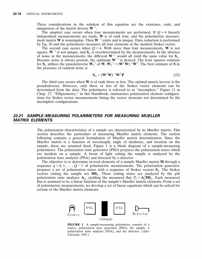
2 2 . 2 1 SAMPLE - MEASURING POLARIMETERS FOR MEASURING MUELLER MATRIX ELEMENTS
The polarization characteristics of a sample are characterized by its Mueller matrix . This section describes the particulars of measuring Mueller matrix elements . The section following contains a general formulation of Mueller matrix determination . Since the Mueller matrix is a function of wavelength , angle of incidence , and location on the sample , these are assumed fixed . Figure 1 is a block diagram of a sample-measuring polarimeter . The polarization state generator (PSG) prepares the polarization states which are incident on a sample . A beam of light exiting the sample is analyzed by the polarization state analyzer (PSA) and detected by a detector .
The objective is to determine several elements of a sample Mueller matrix M through a sequence q 5 0 , 1 , . . . , Q 2 1 of polarimetric measurements . The polarization generator prepares a set of polarization states with a sequence of Stokes vectors S q . The Stokes vectors exiting the sample are MS q . These exiting states are analyzed by the q th polarization state analyzer A q , yielding the measured flux P q 5 A T
q MS q . Each measured flux is assumed to be a linear function of the sample’s Mueller matrix elements . From a set of polarimetric measurements , we develop a set of linear equations which can be solved for certain of the Mueller matrix elements .
FIGURE 1 A sample-measuring polarimeter consists of a source , polarization state generator (PSG) , the sample , a polarization state analyzer (PSA) , and the detector . ( After Chenault , 1 9 9 2 . )
POLARIMETRY 22 .17
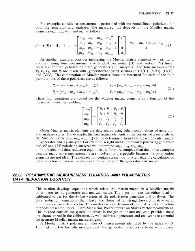
For example , consider a measurement performed with horizontal linear polarizers for both the generator and analyzer . The measured flux depends on the Mueller matrix elements m 0 0 , m 0 1 , m 1 0 , and m 1 1 as follows :
P 5 A T MS 5 1 – 2 [1 1 0 0] 3 m 0 0 m 0 1 m 0 2 m 0 3
m 1 0 m 1 1 m 1 2 m 1 3
m 2 0 m 2 1 m 2 2 m 2 3
m 3 0 m 3 1 m 3 2 m 3 3
4 1 2 3
1 1 0 0 4 5
m 0 0 1 m 0 1 1 m 1 0 1 m 1 1
4 (23)
As another example , consider measuring the Mueller matrix elements m 0 0 , m 0 1 , m 1 0 , and m 1 1 using four measurements with ideal horizontal (H) and vertical (V) linear polarizers for the polarization state generators and analyzers . The four measurements P 0 , P 1 , P 2 , and P 3 are taken with (generator / analyzer) settings of (H / H) , (V / H) , (H / V) , and (V / V) . The combination of Mueller matrix elements measured for each of the four permutations of these polarizers are as follows :
(24) P 0 5 ( m 0 0 1 m 0 1 1 m 1 0 1 m 1 1 ) / 4 , P 1 5 ( m 0 0 1 m 0 1 2 m 1 0 2 m 1 1 ) / 4
P 2 5 ( m 0 0 2 m 0 1 1 m 1 0 2 m 1 1 ) / 4 , P 3 5 ( m 0 0 2 m 0 1 2 m 1 0 1 m 1 1 ) / 4
These four equations are solved for the Mueller matrix elements as a function of the measured intensities , yielding
3 m 0 0
m 0 1
m 1 0
m 1 1
4 5 3 P 0 1 P 1 1 P 2 1 P 3
P 0 1 P 1 2 P 2 2 P 3
P 0 2 P 1 1 P 2 2 P 3
P 0 2 P 1 2 P 2 1 P 3
4 (25)
Other Mueller matrix elements are determined using other combinations of generator and analyzer states . For example , the four matrix elements at the corners of a rectangle in the Mueller matrix h m 0 0 , m 0 i , m j 0 , m j i j can be determined from four measurements using a Ú i -generator and Ú j -analyzer . For example , a right and left circularly polarizing generator and 45 8 and 135 8 polarizing analyzer will determine h m 0 0 , m 0 2 , m 3 0 , m 3 2 j .
In practice , the data reduction equations are far more complex than the above examples because many more measurements are involved , and especially because the polarization elements are not ideal . The next section contains a method to sytematize the calculation of data reduction equations based on calibration data for the generator and analyzer .
2 2 . 2 2 POLARIMETRIC MEASUREMENT EQUATION AND POLARIMETRIC DATA REDUCTION EQUATION
This section develops equations which relate the measurements in a Mueller matrix polarimeter to the generator and analyzer states . The algorithm can use either ideal or calibrated values for the Stokes vectors of the polarization generator and analyzer . The data reduction equations then have the form of a straightforward matrix-vector multiplication on a data vector . This method is an extension of the matrix data reduction methods presented under ‘‘Light-Measuring Polarimeters’’ on Stokes vector measurement . This method corrects for systematic errors in the generator and analyzer , provided these are characterized in the calibration . A well-calibrated generator and analyzer are essential for accurate Mueller matrix measurements .
A Mueller matrix polarimeter takes Q measurements identified by the index q 5 0 , 1 , . . . , Q 2 1 . For the q th measurement , the generator produces a beam with Stokes

22 .18 OPTICAL INSTRUMENTS
vector S q . The beam exiting the sample is analyzed by the polarization analyzer with an analyzer vector A q . The measured flux P q is related to the sample Mueller matrix by
P q 5 A T q MS q 5 [ a q , 0 a q , 1 a q , 2 a q , 3 ] 3
m 0 0 m 0 1 m 0 2 m 0 3
m 1 0 m 1 1 m 1 2 m 1 3
m 2 0 m 2 1 m 2 2 m 2 3
m 3 0 m 3 1 m 3 2 m 3 3
4 3 s q , 0
s q , 1
s q , 2
s q , 3
4 5 O 3
j 5 0 O 3
k 5 0 a q , j m j , k s q , k (26)
This equation is now rewritten as a vector-vector dot product (Azzam , 1978 ; Goldstein , 1992) . First , the Mueller matrix is flattened into a 16 3 1 Mueller y ector M ¢ 5 [ m 0 0 m 0 1 m 0 2 m 0 3 m 1 0 ? ? ? m 3 3 ]
T . A 16 3 1 polarimetric measurement vector W q for the q th measurement is defined as follows
W q 5 [ w q , 0 0 w q , 0 1 w q , 0 2 w q , 0 3 w q , 1 0 ? ? ? w q , 3 3 ] T
5 [ a q , 0 s q , 0 a q , 0 s q , 1 a q , 0 s q , 2 a q , 0 s q , 3 a q , 1 s q , 0 ? ? ? a q , 3 s q , 3 ] T (27)
where w q , j k 5 a q , j s q , k . The q th measured flux from Eq . (25) is rewritten as the dot product
(28)
a q , 0 s q , 0 m 0 , 0
a q , 0 s q , 1 m 0 , 1
a q , 0 s q , 2 m 0 , 2
P q 5 W q ? M ¢ 5 a q , 0 s q , 3 m 0 , 3
a q , 1 s q , 0 m 1 , 0
a q , 1 s q , 1 m 1 , 1
? ? ? ? ? ? a q , 3 s q , 3 m 3 , 3
C DC D The full sequence of measurements is described by the polarimetric measurement matrix W , defined as the Q 3 16 matrix where the q th row is W q . The polarimetric measurement equation relates the measurement vector P to the sample Mueller vector by a matrix- vector multiplication ,
P 5 WM ¢ 5 3 P 0
P 1
? ? ? P Q 2 1
4 5 3 w 0 , 0 0
w 1 , 0 0
? ? ? w Q 2 1 , 0 0
w 0 , 0 1
w 1 , 0 1
w Q 2 1 , 0 1
? ? ?
? ? ?
? ? ?
w 0 , 3 3
w 1 , 3 3
w Q 2 1 , 3 3
4 3 m 0 0
m 0 1
? ? ? m 3 3
4 (29)
If W contains sixteen linearly independent columns , all sixteen elements of the Mueller matrix can be determined . Then , if Q 5 16 , the matrix inverse is unique and the Mueller matrix elements are determined from the polarimetric data reduction equation M ¢ 5 W 2 1 P . More often , Q . 16 , and M ¢ is overdetermined . The optimal (least-squares) polarimetric data reduction equation for M ¢ uses the pseudoinverse W 2 1
P of W , Eq . (21) where W 2 1 P is a
polarimetric data reduction matrix for the polarimeter . The polarimetric data reduction equation is then
M ¢ 5 ( W T W ) 2 1 W T P 5 W 2 1 P P (30)
where W 2 1 P operates on a set of measurements to estimate the Mueller matrix of the
sample .

POLARIMETRY 22 .19
The advantages of this polarimetric measurement equation and polarimetric data reduction equation procedure are as follows . First , this procedure does not assume that the set of states of polarization state generator and analyzer have any particular form . For example , the polarization elements in the generator and analyzer do not need to be rotated in uniform angular increments , but can comprise an arbitrary sequence . Second , the polarization elements are not assumed to be ideal polarization elements or have any particular imperfections . If the Stokes vectors associated with the polarization generator and analyzer are determined through a calibration procedure , the ef fects of nonideal polarization elements are corrected in the data reduction . Third , the procedure readily treats overdetermined measurement sequences (more than sixteen measurements for the full Mueller matrix) , providing a least-squares solution . Finally , a matrix-vector form of data reduction is readily implemented and understood .
The next two sections describe configurations of sample-measuring polarimeter with example data reduction matrices .
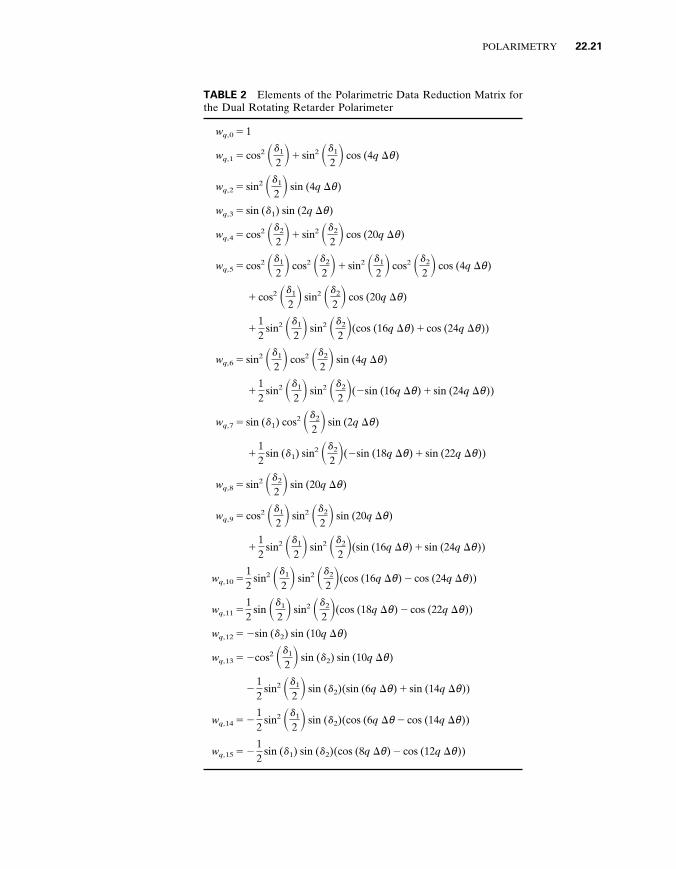
2 2 . 2 3 DUAL ROTATING RETARDER POLARIMETER
The dual rotating retarder Mueller matrix polarimeter is one of the most common Mueller polarimeters . Figure 2 shows the configuration : light from the source passes first through a fixed linear polarizer , then through a rotating linear retarder , the sample , a rotating linear retarder , and finally through a fixed linear polarizer . In the most common configuration , first described by Azzam (1978) , the polarizers are parallel , and the retarders are rotated in angular increments of five-to-one . This five-to-one ratio encodes all 16 Mueller matrix elements onto the amplitudes and phases of 12 frequencies in the detected signal . The detected signal is Fourier analyzed , and the Mueller matrix elements are calculated from the Fourier coef ficients .
This polarimeter design has an important advantage : the polarizers do not move . The polarizer in the generator accepts only one polarization state from the source optics , making the measurement immune to instrumental polarization from the source optics . If the polarizer did rotate , and if the beam incident on it were elliptically polarized , a systematic modulation of intensity would be introduced which would require compensa- tion . Similarly , the polarizer in the analyzer does not rotate ; only one polarization state is transmitted through the analyzing optics and onto the detector . Any diattenuation in the analyzing optics and any polarization sensitivity in the detector will not af fect the measurements .
The data reduction matrix is presented here for a polarimeter with ideal linear retarders with arbitrary retardances d 1 in the generator and d 2 in the analyzer . Optimal values for the retardances are near l / 4 or l / 3 , depending which characteristics of the
FIGURE 2 The dual rotating retarder polarimeter consists of a source , a fixed linear polarizer , a retarder which rotates in steps , the sample , a second retarder which rotates in steps , a fixed linear polarizer , and the detector . This polarimeter measures the full Mueller matrix . It accepts only one polarization state from the source , and transmits only one polarization state to the detector . ( After Chenault , 1 9 9 2 . )
22 .20 OPTICAL INSTRUMENTS
Mueller matrix are chosen for a figure of merit . If d 1 5 d 2 5 π rad , the last row and column of the sample Mueller matrix are not measured . Q measurements are taken , described by index q 5 0 , 1 , . . . , Q 2 1 . The angular orientations of the two retarders for measurement q are θ q , 1 5 q 180 8 / Q and θ q , 2 5 5 q 180 8 / Q . The angular increment between settings of the generator retarder is D θ 5 180 8 / Q . The data reduction matrix is a 16 3 Q matrix which multiplies a Q 3 1 data vector P , yielding the sample Mueller vector M ¢ . Table 2 lists the equations for the elements in each row q of the data reduction matrix assuming ideal polarization elements (Chenault , Pezzaniti , and Chipman , 1992) .
Several data reduction methods have been published to account for additional imperfections in the polarization elements , leading to considerably more elaborate expressions than those presented here . Hauge (1978) developed an algorithm to compensate for the linear diattenuation and linear retardance of the retarders . Goldstein and Chipman (1990) treat five errors , the retardances of the two retarders , and orientation errors of the two retarders and one of the polarizers , in a small angle approximation good for small errors . Chenault , Pezzaniti , and Chipman (1992) extended this method to larger errors .
2 2 . 2 4 INCOMPLETE SAMPLE - MEASURING POLARIMETERS
Incomplete sample-measuring polarimeters do not measure the full Mueller matrix of a sample and thus provide incomplete information regarding the polarization properties of a sample . Often the full Mueller matrix is not needed . For example , many birefringent samples have considerable linear birefringence and minuscule amounts of the other forms of polarization . The magnitude of the birefringence can be measured , assuming all the other polarization ef fects are small , using much simpler configurations than a Mueller matrix polarimeter , such as the circular polariscope (Theocaris and Gdoutos , 1979) . Similarly , homogeneous and isotropic interfaces , such as dielectrics , metals , and thin films , should only display linear diattenuation and linear retardance aligned with the s 2 p planes . These interfaces do not need characterization of their circular diattenuation and circular retardance . Many categories of ellipsometer will characterize such samples without providing the full Mueller matrix (Azzam and Bashara , 1977 , 1987 ; Azzam , 1993) .
2 2 . 2 5 DUAL ROTATING POLARIZER POLARIMETER
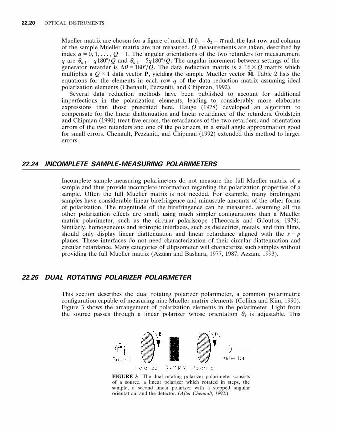
This section describes the dual rotating polarizer polarimeter , a common polarimetric configuration capable of measuring nine Mueller matrix elements (Collins and Kim , 1990) . Figure 3 shows the arrangement of polarization elements in the polarimeter . Light from the source passes through a linear polarizer whose orientation θ 1 is adjustable . This
FIGURE 3 The dual rotating polarizer polarimeter consists of a source , a linear polarizer which rotated in steps , the sample , a second linear polarizer with a stepped angular orientation , and the detector . ( After Chenault , 1 9 9 2 . )
POLARIMETRY 22 .21
TABLE 2 Elements of the Polarimetric Data Reduction Matrix for the Dual Rotating Retarder Polarimeter
w q , 0 5 1
w q , 1 5 cos 2 S d 1
2 D 1 sin 2 S d 1
2 D cos (4 q D θ )
w q , 2 5 sin 2 S d 1
2 D sin (4 q D θ )
w q , 3 5 sin ( d 1 ) sin (2 q D θ )
w q , 4 5 cos 2 S d 2
2 D 1 sin 2 S d 2
2 D cos (20 q D θ )
w q , 5 5 cos 2 S d 1
2 D cos 2 S d 2
2 D 1 sin 2 S d 1
2 D cos 2 S d 2
2 D cos (4 q D θ )
1 cos 2 S d 1
2 D sin 2 S d 2
2 D cos (20 q D θ )
1 1 2
sin 2 S d 1
2 D sin 2 S d 2
2 D (cos (16 q D θ ) 1 cos (24 q D θ ))
w q , 6 5 sin 2 S d 1
2 D cos 2 S d 2
2 D sin (4 q D θ )
1 1 2
sin 2 S d 1
2 D sin 2 S d 2
2 D ( 2 sin (16 q D θ ) 1 sin (24 q D θ ))
w q , 7 5 sin ( d 1 ) cos 2 S d 2
2 D sin (2 q D θ )
1 1 2
sin ( d 1 ) sin 2 S d 2
2 D ( 2 sin (18 q D θ ) 1 sin (22 q D θ ))
w q , 8 5 sin 2 S d 2
2 D sin (20 q D θ )
w q , 9 5 cos 2 S d 1
2 D sin 2 S d 2
2 D sin (20 q D θ )
1 1 2
sin 2 S d 1
2 D sin 2 S d 2
2 D (sin (16 q D θ ) 1 sin (24 q D θ ))
w q , 1 0 5 1 2
sin 2 S d 1
2 D sin 2 S d 2
2 D (cos (16 q D θ ) 2 cos (24 q D θ ))
w q , 1 1 5 1 2
sin S d 1
2 D sin 2 S d 2
2 D (cos (18 q D θ ) 2 cos (22 q D θ ))
w q , 1 2 5 2 sin ( d 2 ) sin (10 q D θ )
w q , 1 3 5 2 cos 2 S d 1
2 D sin ( d 2 ) sin (10 q D θ )
2 1 2
sin 2 S d 1
2 D sin ( d 2 )(sin (6 q D θ ) 1 sin (14 q D θ ))
w q , 1 4 5 2 1 2
sin 2 S d 1
2 D sin ( d 2 )(cos (6 q D θ 2 cos (14 q D θ ))
w q , 1 5 5 2 1 2
sin ( d 1 ) sin ( d 2 )(cos (8 q D θ ) 2 cos (12 q D θ ))

22 .22 OPTICAL INSTRUMENTS
linearly polarized light interacts with the sample and is analyzed by a second linear polarizer whose orientation θ 2 is also adjustable . This polarimeter is incomplete because measurement of the last column of the Mueller matrix requires elliptical states from the polarization generator . Similarly , elliptical analyzers are required in the polarization analyzer to measure the bottom row of the Mueller matrix .
The polarimetric data reduction matrix which follows is for a particular 16- measurement sequence . The most common defects of polarizers have been taken into consideration : less than ideal diattenuation , and transmission of less than unity . The polarizers are characterized by T m a x , the maximum intensity transmittance for a single polarizer , and T m i n , the minimum intensity transmittance , which are associated with orthogonal linear states . Let a 5 (16( T m a x 1 T m i n ) 2 ) 2 1 , b 5 (8( T 2
max 2 T 2 min )) 2 1 and c 5
(4( T m a x 2 T m i n ) 2 ) 2 1 . Sixteen measurements are acquired with the generator polarizer angle θ q , 1 and the analyzer polarizer angle θ q , 2 oriented as follows : θ q , 1 5 (0 8 , 0 8 , 0 8 , 0 8 , 45 8 , 45 8 , 45 8 , 45 8 , 90 8 , 90 8 , 90 8 , 90 8 , 135 8 , 135 8 , 135 8 , 135 8 ) , θ q , 2 5 (0 8 , 45 8 , 90 8 , 135 8 , 0 8 , 45 8 , 90 8 , 135 8 , 0 8 , 45 8 , 90 8 , 135 8 , 0 8 , 45 8 , 90 8 , 135 8 ) . Since only nine Mueller matrix elements are measured , a nine-element Mueller vector is used :
M ¢ 5 [ m 0 0 m 0 1 m 0 2 m 1 0 m 1 1 m 1 2 m 2 0 m 2 1 m 2 2 ] T (31)
The data reduction matrix W 2 1 P which operates on the 16-element measurement vector P
yielding M ¢ is
a a a a a a a a a a a a a a a a
b b b b 0 0 0 0 2 b 2 b 2 b 2 b 0 0 0 0 0 0 0 0 b b b b 0 0 0 0 2 b 2 b 2 b 2 b
b 0 2 b 0 b 0 2 b 0 b 0 2 b 0 b 0 2 b 0 W 2 1
P 5 c 0 2 c 0 0 0 0 0 2 c 0 c 0 0 0 0 0 0 0 0 0 c 0 2 c 0 0 0 0 0 2 c 0 c 0 0 b 0 2 b 0 b 0 2 b 0 b 0 2 b 0 b 0 2 b
0 c 0 2 c 0 0 0 0 0 2 c 0 c 0 0 0 0 0 0 0 0 0 c 0 2 c 0 0 0 0 0 2 c 0 c
C D (32)
The source is assumed to be unpolarized in this equation . Similarly , the detector is assumed to be polarization-insensitive . When this is not the case , the data reduction matrix is readily generalized to incorporate these and other systematic ef fects following the method shown under ‘‘Polarimetric Measurement Equation and Polarimetric Data Reduction Equation . ’’
2 2 . 2 6 NONIDEAL POLARIZATION ELEMENTS
For use in polarimetry , polarization elements require a level of characterization beyond what is normally provided by vendors . For retarders , usually only the linear retardance is specified . For polarizers , usually only the two principal transmittances or the extinction ratio is given . For polarization elements used in critical applications such as polarimetry , this level of characterization is inadequate . In this section , defects of polarization elements
POLARIMETRY 22 .23
are described , and the Mueller calculus is recommended as the most appropriate measure of performance .
2 2 . 2 7 POLARIZATION PROPERTIES OF POLARIZATION ELEMENTS
For ideal polarization elements , the polarization properties are readily defined . For real polarization elements , the precise description of the polarization properties is more complex . The handbook chapter ‘‘Polarizers’’ (Chap . 3) contains an extensive description of the various forms of polarizers and retarders and their characteristics (Bennett 1993) . Polarization elements such as polarizers , retarders , and depolarizers have three general polarization properties : diattenuation , retardance , and depolarization , and a typical element displays some amount of all three . Diattenuation arises when the intensity transmittance of an element is a function of the incident polarization state (Chipman , 1989a) . The diattenuation D of a device is defined in terms of the maximum T m a x and minimum T m i n intensity transmittances ,
D 5 T m a x 2 T m i n
T m a x 1 T m i n (33)
for an ideal polarizer , D 5 1 . When D 5 0 , all incident polarization states are transmitted with equal loss , although the polarization states in general change upon transmission . The quality of a polarizer is often expressed in terms of the related quantity , the extinction ratio E ,
E 5 T m a x
T m i n 5
1 1 D 1 2 D
(34)
Retardance is the phase change a device introduces between its eigenpolarizations (eigenstates) . For a birefringent retarder with refractive indices n 1 and n 2 , and thickness t , the retardance d expressed in radians is
d 5 2 π ( n 1 2 n 2 ) t
l (35)
Depolarization describes the coupling by a device of incident polarized light into depolarized light in the exiting beam . For example , depolarization occurs when light transmits through milk or scatters from clouds . Multimode optical fibers generally depolarize the light . Depolarization is intrinsically associated with scattering and a loss of coherence in the polarization state . A small amount of depolarization is probably associated with the scattered light from all optical components . A depolarization coef ficient e can be defined as the fraction of unpolarized power in the exiting beam when polarized light is incident . e is generally a function of the incident polarization state .
2 2 . 2 8 COMMON DEFECTS OF POLARIZATION ELEMENT
Here we list some common defects found in real polarization elements .
1 . Polarizers have nonideal diattenuation since T m a x , 1 and T m i n . 0 (Bennett , 1993 ; King and Talim , 1971) .

22 .24 OPTICAL INSTRUMENTS
2 . Retarders have the incorrect retardance . Thus , there will be some deviation from a quarter-wave or a half-wave of retardance , for example , because of fabrication errors or a change in wavelength .
3 . Retarders usually have some diattenuation because of dif ferences in absorption coef ficients (dichroism) and due to dif ferent transmission and reflection coef ficients at the interfaces . For example , birefringent retarders have diattenuation due to the dif ference of the Fresnel coef ficients at normal incidence for the two eigenpolarizations since n 1 ? n 2 . This can be reduced by antireflection coatings .
4 . Polarizers usually have some retardance ; there is a dif ference in optical path length between the transmitted (principal) eigenpolarization and the small amount of the extinguished (secondary) eigenpolarization . For example , sheet polarizers and wire-grid polarizers show substantial retardance when the secondary state is not completely extinguished .
5 . The polarization properties vary with angle of incidence ; for example , Glan- Thompson polarizers polarize over only a 4 8 field of view (Bennett , 1994) . Birefringent retarders commonly show a quadratic variation of retardance with angle of incidence which increases along one axis and decreases along the orthogonal axis (Title , 1979 ; Hale and Day , 1988) . For polarizing beam-splitter cubes , the axis of linear polarization rotates for incident light out of its normal plane (the plane defined by the face normals and the beam-splitting interface normal) .
7 . The polarization properties vary with wavelength ; for example , for simple retarders made from a single birefringent plate , the retardance varies approximately linearly with wavelength .
8 . For polarizers , the accepted state and the transmitted state can be dif ferent . Consider a polarizing device formed from a linear polarizer oriented at 0 8 followed by a linear polarizer oriented at 2 8 . Incident light linearly polarized at 0 8 has the highest transmittance for all possible polarization states and is the accepted state . The corresponding exiting beam is linearly polarized at 2 8 , which is the only state exiting the device . In this example , the transmitted state is also an eigenpolarization . This ‘‘rotation’’ between the accepted and transmitted states of a polarizer frequently occurs , for example , when the crystal axes are misaligned in a birefringent polarizing prism assembly such as a Glan-Thompson polarizer .
9 . A nominally ‘‘linear’’ element may be slightly elliptical (have elliptical eigenpolariza- tions) . For example , a quartz linear retarder with the crystal axis misaligned becomes an elliptical retarder . Similarly a circular element may be slightly elliptical . For example , an (inhomogeneous) circular polarizer formed from a linear polarizer followed by a quarter-wave linear retarder at 45 8 [see Eq . (14)] becomes an elliptical polarizer as the retarder’s fast axis is rotated .
10 . The eigenpolarizations of the polarization element may not be orthogonal ; i . e ., a polarizer may transmit linearly polarized light at 0 8 without change of polarization while extinguishing linearly polarized light oriented at 88 8 . Such a polarization element is referred to as inhomogeneous (Shurclif f , 1962 ; Lu and Chipman , 1992) . Sequences of polarization elements , such as optical isolator assemblies , often are inhomogeneous . The circular polarizer in Eq . 14 is inhomogeneous .
11 . A polarization element may depolarize , coupling polarized light into unpolarized light . A polarizer or retarder with a small amount of depolarization , when illuminated by a completely polarized beam , will have a small amount of unpolarized light in the transmitted beam . Such a transmitted beam can no longer be extinguished by an ideal polarizer . Depolarization results from fabrication errors such as surface roughness , bulk scattering , random strains and dislocations , and thin-film microstructure .
12 . Multiply reflected beams and other ‘‘secondary’’ beams may be present with
POLARIMETRY 22 .25
undesired polarization properties . For example , the multiply reflected beams from a birefringent plate have various values for their retardance . Antireflection coatings will reduce this ef fect in one waveband , but may increase these problems with multiple reflections in other wavebands .
The preceding list of polarization element defects is by no means comprehensive . It should serve as a warning to those with demanding applications for polarization elements . In particular , the performance of polarizing beam-splitting cubes have been found to be quite dif ferent from the ideal (Pezzaniti and Chipman , 1991) .
2 2 . 2 9 THE MUELLER MATRIX FOR POLARIZATION COMPONENT CHARACTERIZATION
The Mueller matrix provides the full characterization of a polarization element (Shurclif f , 1962 ; Azzam and Bashara , 1977) . From the Mueller matrix , all of the performance defects listed previously and more are specified . Thus , when one is using polarization elements in critical applications such as polarimetry , it is highly desirable that the Mueller matrix of the elements be known . This is analogous to having the interferogram of a lens to ensure that it is of suitable quality for incorporation into a critical imaging system .
The optics community has been very slow to adopt Mueller matrices for the testing of optical components and optical systems , delaying a broad understanding of how real polarization elements actually perform . An impediment to the widespread acceptance of Mueller matrices for polarization element qualification has been that the polarization properties associated with a Mueller matrix (the diattenuation , retardance , and depolariza- tion) are not easily ‘‘extracted’’ from the Mueller matrix . Thus , while the operational definition of the Mueller matrix , Eq . (10) , is straightforward , determining the diattenua- tion , retardance , and depolarization from an experimentally determined Mueller matrix is a complex process (Gil and Bernabeau , 1987) . This is described later in this chapter .
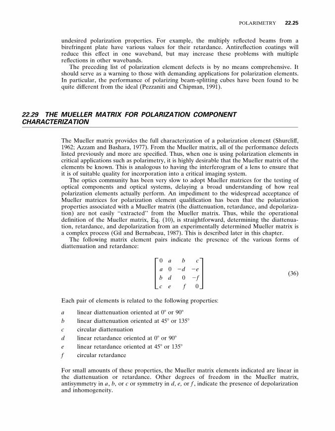
The following matrix element pairs indicate the presence of the various forms of diattenuation and retardance :
3 0 a
b
c
a
0 d
e
b
2 d
0 f
c
2 e
2 f
0 4 (36)
Each pair of elements is related to the following properties :
a linear diattenuation oriented at 0 8 or 90 8
b linear diattenuation oriented at 45 8 or 135 8
c circular diattenuation d linear retardance oriented at 0 8 or 90 8
e linear retardance oriented at 45 8 or 135 8
f circular retardance
For small amounts of these properties , the Mueller matrix elements indicated are linear in the diattenuation or retardance . Other degrees of freedom in the Mueller matrix , antisymmetry in a , b , or c or symmetry in d , e , or f , indicate the presence of depolarization and inhomogeneity .
22 .26 OPTICAL INSTRUMENTS
2 2 . 3 0 APPLICATIONS OF POLARIMETRY
Polarimetry has found application in nearly all areas of science and technology with several tens of thousands of papers detailing various applications . The following summarizes a few of the principal applications and introduces some of the books , reference works , and review papers which provide gateways to the various applications .
Ellipsometry
Ellipsometry is the application of polarimetry for determining the optical properties of surfaces and interfaces . Example applications are refractive indices and thin-film thickness determination , and investigations of processes at surfaces such as contamination and corrosion . In this Handbook , Chap . 27 , ‘‘Ellipsometry , ’’ by Azzam treats the fundamen- tals . A more extensive treatment is found in the textbook by Azzam and Bashara (1979 and 1986) which presents the mathematical fundamentals of polarization , determination of the properties of thin films , polarimetric instrumentation , and a myriad of applications . Azzam (1991) is a recent collection of historical papers . Calculation of the polarization properties of thin films is given a detailed presentation by Dobrowolski (1994) in Chap . 43 of Vol . I of this Handbook , and also in the text by Macleod (1986) .
Spectropolarimetry for Chemical Applications
Spectropolarimeters are spectrometers which incorporate polarimeters for the purpose of measuring polarization properties as a function of wavelength . Whereas spectrometers measure transmission or reflectance as a function of wavelength , a spectropolarimeter also may measure dichroism (diattenuation) , linear birefringence (linear retardance) , optical activity (circular retardance) , or depolarization , all as spectra . In physical chemistry , spectra of the linear dichroism and the linear retardance of a molecule permit the determination of the orientation of the electric dipole moment in three dimensions . Similarly , circular dichroism and optical activity provide information on the orbital magnetic moment . Schellman and Jensen (1987) and Johnson (1987) provide comprehen- sive surveys of the spectropolarimetry of oriented molecules and interpretation of the data in terms of molecular structure . The volumes by Michl and Thulstrup (1986) , Samori and Thulstrup (eds . ) (1988) , and by Kliger , Lewis , and Randall (1990) cover the basics of polarimetry with an emphasis on spectroscopy with polarized light and interpretation of the resulting data . Texts and reviews on optical activity include the following : Jirgensons (1973) , Mason (ed . ) (1978) , Mason (1982) , Thulstrup (1982) , Barron (1986) , and Laktakia (1990) . Chenault (1992) contains a survey of spectropolarimetric instrumentation .
Remote Sensing
Polarimetry has become an important technique in remote sensing , since it augments the limited information available from spectrometric techniques . Polarization in the scattered light from the earth has many subtle characteristics . The sunlight which illuminates the earth is essentially unpolarized , but the scattered light has a surprisingly large degree of polarization , which is mostly linear polarization (Egan , 1985 ; Konnen , 1985 ; Coulson , 1988 ; Coulson , 1989 ; Egan , 1992) . Visible light scattered from forest canopy , cropland , meadows , and similar features frequently has a degree of polarization of 20 percent or greater in the visible (Curran , 1982 ; Duggin , 1989) . Light reflecting from mudflats and water often has a degree of polarization of 50 percent or higher , particularly for light incident near

POLARIMETRY 22 .27
Brewster’s angle . Light scattered from clouds is nearly unpolarized (Konnen , 1985 ; Coulson , 1988) . The magnitude of the degree of linear polarization depends on many variables , including the angle of incidence , the angle of scatter , the wavelength , and the weather . The polarization from a site varies from day to day even if the angles of incidence and scatter remain the same ; these variations are caused just by changes in the earth’s vegetation , cloud cover , humidity , rain , and standing water . Polarization is complex to interpret but it conveys a great deal of useful information .
Astronomical Polarimetry
The polarization of light from astronomical bodies conveys considerable information regarding their physical state—information that generally cannot be acquired by any other means . Gehrels (1974) compiles information regarding the polarization of plants , stars , and other astronomical objects . Polarimetry is the principle technique for determining solar magnetic fields . Solar vector magnetographs are imaging polarimeters combined with narrowband tunable spectral filters which measure Zeeman splitting in magnetically active ions in the solar atmosphere , from which the magnetic fields can be determined . November (1991) is a recent survey of instrumentation and ongoing measurement programs for solar magnetic field study .
Polarization Light Scattering
Polarization light scattering is the application of polarimetry to scattered light (Van de Hulst , 1957 ; Stover , 1990) . The scattering characteristics of a sample are generally described by its bidirectional reflectance distribution function , BRDF ( a , b , g , d , l ) , which is the ratio of the scattered flux in a particular direction ( g , d ) to the flux of an incident beam from direction ( a , b ) . The BRDF function contains no polarization information , but is the m 0 0 element of the Mueller matrix relating the incident and scattered beams . The BRDF can be generalized to a Mueller bidirectional reflectance distribution function , or MBRDF ( a , b , g , d , l ) , which is the Mueller matrix relating arbitrary incident and scattered beams . Scattered light is often a sensitive indicator to surface conditions ; a small amount of surface roughness may reduce the specular power by less than a percent while increasing the scattered power by orders of magnitude . The retardance , diattenuation , and depolarization of the scattered light similarly provide sensitive indicators of light- scattering conditions , such as uniformity of refractive index , orientation of surface defects , texture , strain and birefringence at an interface , subsurface damage , coating microstruc- ture , and the degree of multiple scattering .
Optical and Polarization Metrology
Polarimetry is useful in optical metrology for measuring the instrumental polarization of optical systems and for characterizing optical and polarization components . Optical systems , both common and exotic , modify the polarization state of light due to the reflections , refractions , and other interactions with optical materials . Each ray path through the optical system can be characterized by its polarization matrix (Chipman , 1989a ; Chipman , 1989b) . Polarization ray tracing is the technique of calculating the polarization matrices for ray paths from the optical and coating prescriptions (Waluschka , 1989 ; Bruegge , 1989 ; Wolf f and Kurlander , 1990) . Dif fraction image formation of polarization-aberrated beams is then handled by vector extensions to dif fraction theory (Kuboda and Inoue ̀ , 1959 ; Urbanczyk , 1984 ; Urbanczyk , 1986 ; McGuire and Chipman , 1990 ; McGuire and Chipman , 1991 ; Mansuripur , 1991) . Polarimeters , particularly imaging

22 .28 OPTICAL INSTRUMENTS
polarimeters , are used to measure the Mueller matrices of ray paths through optical systems determining the polarization aberrations . These polarization aberrations fre- quently have the same functional forms as the geometrical aberrations , since they arise from similar geometrical considerations (Chipman , 1987 ; McGuire and Chipman , 1987 , 1989 , 1990a , 1990b , 1991 ; Hansen , 1988 ; Chipman and Chipman , 1989) . Several con- ferences have surveyed these areas (Chipman , 1988 ; Chipman , 1989c ; Goldstein and Chipman , 1992) .
Radar Polarimetry
Polarimetric measurements are a standard and highly evolved technique in radar with broad application (Poelman and Guy , 1985 ; Holm , 1987 ; van Zyl and Zebker , 1990) . Although radar is outside the scope of this handbook , several references to the radar literature are included since the optical community can greatly benefit from advances in radar polarimetry . The text by Mott (1992) develops the polarization properties of antennas and the techniques of radar polarimetry . Fundamental analyses of the Mueller matrix have been performed by Huynen (1965) and Kennaugh (1951) , both of which have found broad application in the interpretation of radar polarization signatures . Morris and Chipman (eds . ) (1990) and Boerner and Mott (eds . ) (1992) are proceedings from meetings specifically intended to provide an exchange between the optical polarimetry and radar polarimetry communities .
2 2 . 3 1 INTERPRETATION OF MUELLER MATRICES
The Mueller matrix is defined as a matrix which transforms incident Stokes vectors into exiting Stokes vectors with each element seen as a coupling between corresponding Stokes vector elements . Despite this simple and elegant definition , the polarization properties associated with the Mueller matrix—the diattenuation , retardance , and depolarization— are not readily apparent from the matrix for two reasons . First , the Stokes vector has an unusual coordinate system in which the dif ferent elements do not represent orthogonal polarization components . Instead , positive and negative values on each component separately represent orthogonal polarization components . Second , the phenomenon of depolarization greatly complicates the matrix properties . It is not possible to analyze real arbitrary Mueller matrices measured by polarimeters without considering three tricky topics : physical realizability , depolarization , and inhomogeneity .
2 2 . 3 2 DIATTENUATION AND POLARIZATION SENSITIVITY
The intensity transmittance T for a given matrix M and incident polarization state S is defined as the ratio of exiting flux s 9 0 to incident flux s 0 ,
T ( MS ) 5 s 9 0
s 0 5
m 0 0 s 0 1 m 0 1 s 1 1 m 0 2 s 2 1 m 0 3 s 3
s 0 (37)
The intensity transmittance averaged over all incident polarization states is T a v g 5 m 0 0 . The maximum T m a x and minimum T m i n intensity transmittances are
T m a x 5 m 0 0 1 4 m 2 01 1 m 2
02 1 m 2 03 , T m i n 5 m 0 0 2 4 m 2
01 1 m 2 02 1 m 2
03 (38)

POLARIMETRY 22 .29
and are associated with the unnormalized incident states
S m a x 5 3 4 m 2
01 1 m 2 03 1 m 2
03
m 0 1
m 0 2
m 0 3
4 S m i n 5 3 4 m 2
01 1 m 2 03 1 m 2
03
2 m 0 1
2 m 0 2
2 m 0 3
4 (39)
The incident Stokes vectors of maximum S m a x and minimum S m i n intensity transmittance are always orthogonal . The term diattenuation refers to the two attenuations associated with these two orthogonal states . The diattenuation D ( M ) of a Mueller matrix is a measure of the variation of intensity transmittance with incident polarization state ,
D ( M ) 5 T m a x 2 T m i n
T m a x 1 T m i n 5
4 m 2 01 1 m 2
02 1 m 2 03
m 0 0 (40)
When D 5 1 , the device is an ideal analyzer ; it completely blocks one polarization component of the incident light , and only one Stokes vector exits the device . If this device is also nondepolarizing , then M represents a polarizer . When D 5 0 , all incident states have the same intensity transmittance : the device may be nonpolarizing , depolarizing , or a pure retarder . Diattenuation is also referred to as polarization sensiti y ity . Linear polarization sensiti y ity or linear diattenuation LD ( M ) characterizes the variation of intensity transmittance with incident linear polarization states :
LD ( M ) 5 4 m 2
01 1 m 2 02
m 0 0 (41)
Linear polarization sensitivity is frequently specified as a performance parameter in remote sensing systems designed to measure incident power independently of any linearly polarized component present in scattered earth-light (Maymon and Chipman , 1991) . Note that LD ( M ) 5 1 specifies that M is a linear analyzer ; M is not necessarily a linear polarizer , but may represent a linear polarizer followed by some other polarization element . Diattenuation in (fiber optical) components and systems is often characterized by the polarization dependent loss , given in decibels :
PDL ( M ) 5 10 Log 1 0 T m a x
T m i n (42)
2 2 . 3 3 POLARIZANCE
The polarizance P ( M ) is the degree of polarization of the transmitted light when unpolarized light is incident (Bird and Shurclif f , 1959 ; Shurclif f , 1962) .
P ( M ) 5 4 m 2
10 1 m 2 20 1 m 2
30
m 0 0 (43)
The Stokes vector of the exiting light S P is specified by the first column of M ,
S P ( M ) 5 [ m 0 0 m 1 0 m 2 0 m 3 0 ] T (44)
and is not generally equal to S m a x when inhomogeneity or depolarization is present .

22 .30 OPTICAL INSTRUMENTS
2 2 . 3 4 PHYSICALLY REALIZABLE MUELLER MATRICES
Mueller matrices form a subset of the four-by-four real matrices . A four-by-four real matrix is not a physically realizable Mueller matrix if it can operate on an incident Stokes vector to produce a vector with degree of polarization greater than one ( s 2
0 , s 2 1 1 s 2
2 1 s 2 3 ) ,
which represents a physically unrealizable polarization state . Similarly , a Mueller matrix cannot output a state with negative flux . Conditions for physical realizability have been studied extensively in the literature , and many necessary conditions have been published (Hovenier , van de Hulst , and van der Mee , 1986 ; Barakat , 1987 ; Cloude , 1989 ; Girgel , 1991 ; Xing , 1992 ; Kumar and Simon , 1992 ; van der Mee and Hovenier , 1992 ; Kostinski , Givens , and Kwiatkowski) . A set of suf ficient conditions for physical realizability is not known to this author . The following four necessary conditions for physical realizability are among the more general of those published :
1 . Tr ( MM T ) # 4 m 2 00
2 . m 0 0 $ u m i j u 3 . m 2
00 $ b 2
4 . ( m 0 0 2 b ) 2 $ O 3
j 5 1 S m 0 , j 2 O 3
k 5 1 m j , k a k D
where b 5 4 m 2 01 1 m 2
02 1 m 2 03 , a j 5 m 0 , j / b , and Tr indicates the trace of a matrix .
Another condition for physical realizability is that the matrix can be expressed as a sum of nondepolarizing Mueller matrices . The Mueller matrix for a passive device T m a x # 1 , a device without gain , must satisfy the relation T m a x 5 m 0 0 1 4 m 2
01 1 m 2 02 1 m 2
03 # 1 . In the 16-dimensional space of Mueller matrices , the matrices for ideal polarizers , ideal
retarders , and other nondepolarizing elements lie on the boundary between the physically realizable Mueller matrices and the unrealizable matrices . Thus , a small amount of noise in the measurement of a Mueller matrix for a polarizer or retarder may yield a marginally unrealizable matrix .
2 2 . 3 5 DEPOLARIZATION
Depolarization is the coupling of polarized into unpolarized light . If an incident state is polarized and the exiting state has a degree of polarization less than one , then the sample has depolarization . Consider three Mueller matrices of the following forms :
ID 5 3 1 0 0 0 0 0 0 0 0 0 0 0 0 0 0 0
4 PD 5 3 1 0 0 0
0 a
0 0
0 0 a
0
0 0 0 a 4 VD 5 3
1 0 0 0
0 a
0 0
0 0 b
0
0 0 0 c 4 (45)
Matrix ID is the ideal depolarizer ; only unpolarized light exits the depolarizer . Matrix PD is the partial depolarizer ; all fully polarized incident states exit with their incident polarization ellipse , but with a degree of polarization DOP ( PD ) 5 a . Matrix PD represents a variable partial depolarizer ; the degree of polarization of the exiting light is a function of the incident state . Physically , depolarization is closely related to scattering and usually has its origin in retardance or diattenuation which is rapidly varying in time , space , or wavelength .
The amount of depolarization is a function of the incident state , and is defined for polarized incident states as 1 2 DOP h MS j . To describe the depolarization characteristics
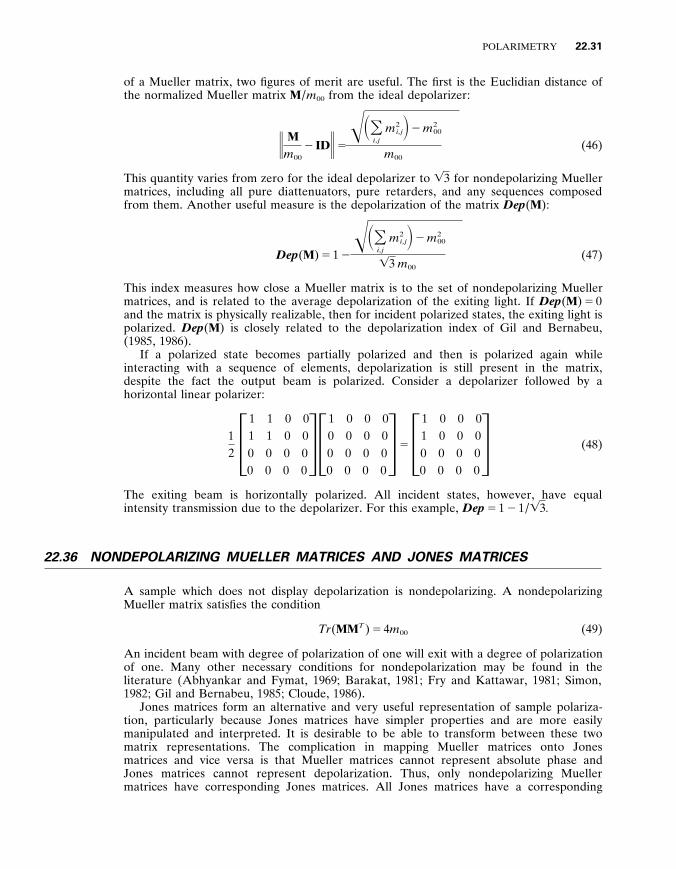
POLARIMETRY 22 .31
of a Mueller matrix , two figures of merit are useful . The first is the Euclidian distance of the normalized Mueller matrix M / m 0 0 from the ideal depolarizer :
I M m 0 0
2 ID I 5 – S O
i ,j m 2
i ,j D 2 m 2 00
m 0 0 (46)
This quantity varies from zero for the ideal depolarizer to 4 3 for nondepolarizing Mueller matrices , including all pure diattenuators , pure retarders , and any sequences composed from them . Another useful measure is the depolarization of the matrix Dep ( M ) :
Dep ( M ) 5 1 2 – S O
i ,j m 2
i ,j D 2 m 2 00
4 3 m 0 0 (47)
This index measures how close a Mueller matrix is to the set of nondepolarizing Mueller matrices , and is related to the average depolarization of the exiting light . If Dep ( M ) 5 0 and the matrix is physically realizable , then for incident polarized states , the exiting light is polarized . Dep ( M ) is closely related to the depolarization index of Gil and Bernabeu , (1985 , 1986) .
If a polarized state becomes partially polarized and then is polarized again while interacting with a sequence of elements , depolarization is still present in the matrix , despite the fact the output beam is polarized . Consider a depolarizer followed by a horizontal linear polarizer :
1 2 3
1 1 0 0 1 1 0 0 0 0 0 0 0 0 0 0
4 3 1 0 0 0 0 0 0 0 0 0 0 0 0 0 0 0
4 5 3 1 0 0 0 1 0 0 0 0 0 0 0 0 0 0 0
4 (48)
The exiting beam is horizontally polarized . All incident states , however , have equal intensity transmission due to the depolarizer . For this example , Dep 5 1 2 1 / 4 3 .
2 2 . 3 6 NONDEPOLARIZING MUELLER MATRICES AND JONES MATRICES
A sample which does not display depolarization is nondepolarizing . A nondepolarizing Mueller matrix satisfies the condition
Tr ( MM T ) 5 4 m 0 0 (49)
An incident beam with degree of polarization of one will exit with a degree of polarization of one . Many other necessary conditions for nondepolarization may be found in the literature (Abhyankar and Fymat , 1969 ; Barakat , 1981 ; Fry and Kattawar , 1981 ; Simon , 1982 ; Gil and Bernabeu , 1985 ; Cloude , 1986) .
Jones matrices form an alternative and very useful representation of sample polariza- tion , particularly because Jones matrices have simpler properties and are more easily manipulated and interpreted . It is desirable to be able to transform between these two matrix representations . The complication in mapping Mueller matrices onto Jones matrices and vice versa is that Mueller matrices cannot represent absolute phase and Jones matrices cannot represent depolarization . Thus , only nondepolarizing Mueller matrices have corresponding Jones matrices . All Jones matrices have a corresponding
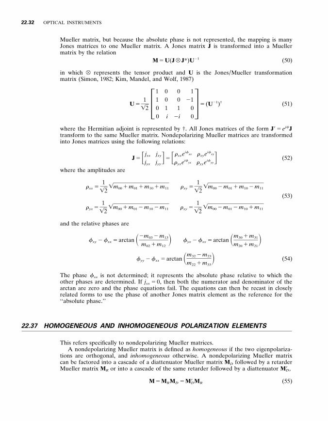
22 .32 OPTICAL INSTRUMENTS
Mueller matrix , but because the absolute phase is not represented , the mapping is many Jones matrices to one Mueller matrix . A Jones matrix J is transformed into a Mueller matrix by the relation
M 5 U ( J ̂ J *) U 2 1 (50)
in which ̂ represents the tensor product and U is the Jones / Mueller transformation matrix (Simon , 1982 ; Kim , Mandel , and Wolf , 1987)
U 5 1
4 2 3 1 1 0 0
0 0 1 i
0 0 1
2 i
1 2 1
0 0 4 5 ( U 2 1 ) † (51)
where the Hermitian adjoint is represented by † . All Jones matrices of the form J 9 5 e j f J transform to the same Mueller matrix . Nondepolarizing Mueller matrices are transformed into Jones matrices using the following relations :
J 5 F j x x
j y x
j x y
j y y G 5 F r x x e i f
x x
r y x e i f y x
r x y e i f x y
r y y e i f y y G (52)
where the amplitudes are
(53)
r x x 5 1
4 2 4 m 0 0 1 m 0 1 1 m 1 0 1 m 1 1 r x y 5
1 4 2
4 m 0 0 2 m 0 1 1 m 1 0 2 m 1 1
r y x 5 1
4 2 4 m 0 0 1 m 0 1 2 m 1 0 2 m 1 1 r x y 5
1 4 2
4 m 0 0 2 m 0 1 2 m 1 0 1 m 1 1
and the relative phases are
f x y 2 f x x 5 arctan S 2 m 0 3 2 m 1 3
m 0 2 1 m 1 2 D f y x 2 f x x 5 arctan S m 3 0 1 m 3 1
m 2 0 1 m 2 1 D
f y y 2 f x x 5 arctan S m 3 2 2 m 2 3
m 2 2 1 m 3 3 D (54)
The phase f x x is not determined ; it represents the absolute phase relative to which the other phases are determined . If j x x 5 0 , then both the numerator and denominator of the arctan are zero and the phase equations fail . The equations can then be recast in closely related forms to use the phase of another Jones matrix element as the reference for the ‘‘absolute phase . ’’
2 2 . 3 7 HOMOGENEOUS AND INHOMOGENEOUS POLARIZATION ELEMENTS
This refers specifically to nondepolarizing Mueller matrices . A nondepolarizing Mueller matrix is defined as homogeneous if the two eigenpolariza-
tions are orthogonal , and inhomogeneous otherwise . A nondepolarizing Mueller matrix can be factored into a cascade of a diattenuator Mueller matrix M D followed by a retarder Mueller matrix M R or into a cascade of the same retarder followed by a diattenuator M 9 D ,
M 5 M R M D 5 M 9 D M R (55)
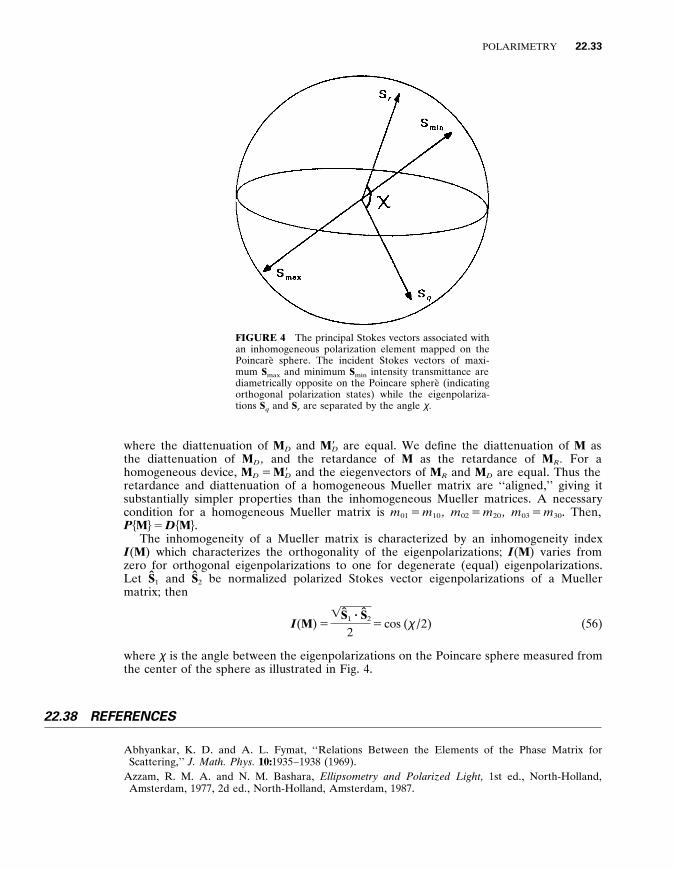
POLARIMETRY 22 .33
FIGURE 4 The principal Stokes vectors associated with an inhomogeneous polarization element mapped on the Poincare ̀ sphere . The incident Stokes vectors of maxi- mum S m a x and minimum S m i n intensity transmittance are diametrically opposite on the Poincare sphere ̀ (indicating orthogonal polarization states) while the eigenpolariza- tions S q and S r are separated by the angle χ .
where the diattenuation of M D and M 9 D are equal . We define the diattenuation of M as the diattenuation of M D , and the retardance of M as the retardance of M R . For a homogeneous device , M D 5 M 9 D and the eiegenvectors of M R and M D are equal . Thus the retardance and diattenuation of a homogeneous Mueller matrix are ‘‘aligned , ’’ giving it substantially simpler properties than the inhomogeneous Mueller matrices . A necessary condition for a homogeneous Mueller matrix is m 0 1 5 m 1 0 , m 0 2 5 m 2 0 , m 0 3 5 m 3 0 . Then , P h M j 5 D h M j .
The inhomogeneity of a Mueller matrix is characterized by an inhomogeneity index I ( M ) which characterizes the orthogonality of the eigenpolarizations ; I ( M ) varies from zero for orthogonal eigenpolarizations to one for degenerate (equal) eigenpolarizations . Let S ̂ 1 and S ̂ 2 be normalized polarized Stokes vector eigenpolarizations of a Mueller matrix ; then
I ( M ) 5 4 S ̂ 1 ? S ̂ 2
2 5 cos ( χ / 2) (56)
where χ is the angle between the eigenpolarizations on the Poincare sphere measured from the center of the sphere as illustrated in Fig . 4 .
2 2 . 3 8 REFERENCES
Abhyankar , K . D . and A . L . Fymat , ‘‘Relations Between the Elements of the Phase Matrix for Scattering , ’’ J . Math . Phys . 10 : 1935 – 1938 (1969) .
Azzam , R . M . A . and N . M . Bashara , Ellipsometry and Polarized Light , 1st ed ., North-Holland , Amsterdam , 1977 , 2d ed ., North-Holland , Amsterdam , 1987 .

22 .34 OPTICAL INSTRUMENTS
Azzam , R . M . A ., ‘‘Photopolarimetric Measurement of the Mueller Matrix by Fourier Analysis of a Single Detected Signal , ’’ Opt . Lett . 2 : 148 – 150 (1978) .
Azzam , R . M . A ., ‘‘Arrangement of Four Photodetectors for Measuring the State of Polarization of Light , ’’ Opt . Lett . 10 : 309 – 311 (1985) .
Azzam , R . M . A ., I . J . Elminyawi , and A . M . El-Saba , ‘‘General Analysis and Optimization of the Four-detector Photopolarimeter , ’’ J . Opt . Soc . Am . A , 5 : 681 – 689 (1988) .
Azzam , R . M . A ., ‘‘Instrument Matrix of the Four-detector Photopolarimeter : Physical Meaning of its Rows and Columns and Constraints on its Elements , ’’ J . Opt . Soc . Am . A 7 : 87 – 91 (1990) .
Azzam , R . M . A . (ed . ) , ‘‘Ellipsometry , ’’ Soc . Photo - Opt . Instrum . Eng . Milestone Series , MS27 (1991) . Azzam , R . M . A ., ‘‘Ellipsometry , ’’ in M . Bass (ed . ) , Handbook of Optics , vol . 2 , 2d ed ., McGraw-Hill , New York , 1994 .
Barakat , R ., ‘‘Bilinear Constraints Between Elements of the 4 3 4 Mueller-Jones Transfer Matrix of Polarization Theory , ’’ Opt . Commun . 38 : 159 – 161 (1981) .
Barakat , R ., ‘‘Conditions for the Physical Realizability of Polarization Matrices Characterizing Passive Systems , ’’ J . Mod . Opt . 34 : 1535 – 1544 (1987) .
Barron , L . D ., Molecular Light Scattering and Optical Acti y ity , Cambridge University Press , New York , 1982 .
Bennett , J . M ., ‘‘Polarization , ’’ in M . Bass (ed . ) , Handbook of Optics , vol . 2 , 2d ed ., McGraw-Hill , New York , 1994 .
Bennett , J . M ., ‘‘Polarizers , ’’ in M . Bass (ed . ) , Handbook of Optics , vol . 2 , 2d ed ., McGraw-Hill , New York , 1994 .
Bird , G . R . and Shurclif f , W . A ., ‘‘Pile-of-plates Polarizers for the Infrared : Improvement in Analysis and Design , ’’ J . Opt . Soc . Am . 49 : 235 – 240 (1959) .
Boerner , W . and H . Mott (eds . ) , ‘‘Radar Polarimetry , ’’ Proc . Soc . Photo - Opt . Instrum . Eng . 1747 (1992) .
Bruegge , T . J ., ‘‘Analysis of Polarization in Optical Systems , ’’ in R . A . Chipman (ed . ) , ‘‘Polarization Considerations for Optical Systems II , ’’ Proc . Soc . Photo - Opt . Instrum . Eng . 1166 : 165 – 176 (1989) .
Chenault , D . B ., ‘‘Infrared Spectropolarimetry , ’’ Ph . D . dissertation , University of Alabama in Huntsville , 1992 .
Chenault , D . B ., J . L . Pezzaniti , and R . A . Chipman , ‘‘Mueller Matrix Algorithms , ’’ in D . Goldstein and R . Chipman (eds . ) , ‘‘Polarization Analysis and Measurement , ’’ Proc . Soc . Photo - Opt . Instrum . Eng . 1746 : 231 – 246 (1992) .
Chipman , R . A ., ‘‘Polarization Aberrations , ’’ Ph . D . Dissertation , Optical Sciences , University of Arizona , 1987 .
Chipman , R . A . (ed . ) , ‘‘Polarization Considerations for Optical Systems , ’’ Proc . Soc . Photo - Opt . Instrum . Eng . 891 (1988) .
Chipman , R . A ., ‘‘Polarization Analysis of Optical System , ’’ Opt . Eng . 28 : 90 – 99 (1989a) . Chipman , R . A ., ‘‘Polarization Analysis of Optical Systems II , ’’ in Russell A . Chipman (ed . ) , ‘‘Polarization Considerations for Optical Systems II , ’’ Proc . Soc . Photo - Opt . Instrum . Eng . 1166 : 79 – 99 (1989b) .
Chipman , R . A . (ed . ) , ‘‘Polarization Considerations for Optical Systems II , ’’ Proc . Soc . Photo - Opt . Instrum . Eng . 1166 (1989c) .
Chipman , R . A . and L . J . Chipman , ‘‘Polarization Aberration Diagrams , ’’ Opt . Eng . 28 : 100 – 106 (1989) .
Cloude , S . R ., ‘‘Group Theory and Polarisation Algebra , ’’ Optik 75 : 26 – 36 (1986) . Cloude , S . R ., ‘‘Conditions for the Physical Realisability of Matrix Operators in Polarimetry , ’’ Proc . Soc . Photo - Opt . Instrum . Eng . 1166 : 177 – 185 (1989) .
Collett , E ., Polarized Light , Marcel Dekker , Inc ., New York , 1992 . Collins , R . W . and Y . -T . Kim , ‘‘Ellipsometry for Thin-film and Surface Analysis , ’’ Ann . Chem . 62 : 887a – 900a (1990) .
Coulson , K . L ., Polarization and Intensity of Light in the Atmosphere , A . Deepak , Hampton , Va ., 1988 .
Coulson , K . L ., ‘‘Polarization of Light in the Natural Environment , ’’ in R . Chipman (ed . ) , Polarization Considerations for Optical Systems II 1166 : 2 – 10 (1989) .

POLARIMETRY 22 .35
Curran , P . J ., ‘‘Polarized Visible Light as an Aid to Vegetation Classification , ’’ Remote Sensing of the En y ironment 12 : 491 – 499 (1982) .
Dobrowolski , G ., ‘‘Optical Properties of Films and Coatings , ’’ in M . Bass (ed . ) , Handbook of Optics , Vol . 1 , 2d ed ., McGraw-Hill , New York , 1994 .
Duggin , M . J ., S . A . Israel , V . S . Whitehead , J . S . Myers , and D . R . Robertson , ‘‘Use of Polarization Methods in Earth Resource Investigations , ’’ in R . Chipman (ed . ) , Polarization Considerations for Optical Systems II 1166 : 42 – 51 (1989) .
Egan , W . G ., Photometry and Polarization in Remote Sensing , Elsevier , New York , 1985 . Egan , W . (ed . ) , ‘‘Polarization in Remote Sensing , ’’ Proc . Soc . Photo - Opt . Instrum . Eng . 1748 (1992) . Fry , E . S . and G . W . Kattawar , ‘‘Relationships Between Elements of the Stokes Matrix , ’’ Appl . Opt . 20 : 2811 – 2814 (1981) .
Gehrels , T . (ed . ) , Planets , Stars , and Nebulae Studied with Polarimetry , Univ . Arizona Press , Tucson , 1974 .
Gerrard , A . and J . M . Burch , Introduction to Matrix Methods in Optics , Wiley , London , 1975 . Gil , J . J . and E . Bernabeu , ‘‘A Depolarization Criterion in Mueller Matrices , ’’ Opt . Acta 32 : 259 – 261 (1985) .
Gil , J . J . and E . Bernabeu , ‘‘Depolarization and Polarization Indices of an Optical System , ’’ Opt . Acta 33 : 185 – 189 (1986) .
Gil , J . J . and E . Bernabeu , ‘‘Obtainment of the Polarizing and Retardation Parameters of a Non-depolarizing Optical System from the Polar Decomposition of Its Mueller Matrix , ’’ Optik 76 : 67 – 71 (1987) .
Girgel , S . S ., ‘‘Structure of the Mueller Matrices of Depolarized Optical Systems , ’’ So y . Phys . Crystallogr . 36 : 890 – 891 (1991) .
Goldstein , D . H ., ‘‘Mueller Matrix Dual-rotating Retarder Polarimeter , ’’ Appl . Opt . 31 , 6676 – 6683 (1992) .
Goldstein , D . H . and R . A . Chipman , ‘‘Error Analysis of a Mueller Matrix Polarimeter , ’’ J . Opt . Soc . Am . A7 : 693 – 700 (1990) .
Goldstein , D . H . and R . A . Chipman (eds . ) , ‘‘Polarization Analysis and Measurement , ’’ Proc . Soc . Photo - Opt . Instrum . Eng . 1745 (1992) .
Hale , P . D . and G . W . Day , ‘‘Stability of Birefringent Linear Retarders (Waveplates) , ’’ Appl . Opt . 27 : 5146 – 5153 (1988) .
Hansen , E . W ., ‘‘Overcoming Polarization Aberrations in Microscopy , ’’ in R . Chipman (ed . ) , ‘‘Polarization Considerations for Optical Systems , ’’ Proc . Soc . Photo - Opt . Instrum . Eng . 891 : 190 – 197 (1988) .
Hauge , P . S ., ‘‘Mueller Matrix Ellipsometry with Imperfect Compensators , ’’ J . Opt . Soc . Am . 68 : 1519 – 1528 (1978) .
Holm , W . A ., ‘‘Polarimetric Fundamentals and Techniques , ’’ in J . L . Eaves and E . K . Reedy (eds . ) , Principles of Modern Radar , Van Nostrand Reinhold , New York , 1987 .
Hovenier , J . W ., H . C . van de Hulst , and C . V . M . van der Mee , ‘‘Conditions for the Elements of the Scattering Matrix , ’’ Astron . Astrophys . 157 : 301 – 310 (1986) .
Huynen , J . R ., ‘‘Measurement of the Target Scattering Matrix , ’’ Proc . IEEE 53 (8) : 936 – 946 (1965) . Jirgensons , B ., Optical Acti y ity of Proteins and Other Macromolecules , Springer-Verlag , New York , 1973 .
Johnson , W . C . Jr ., ‘‘The Circular Dichroism of Carbohydrates , ’’ Ad y ances in Carbohydrate Chemistry and Biochemistry 45 : 73 – 124 (1987) .
Kennaugh , E . M ., ‘‘Ef fects of Type of Polarization on Echo Characteristics , ’’ Report No . 389 – 9 , Antenna Laboratory , Ohio State University , 1951 .
Kim , K ., L . Mandel , and E . Wolf , ‘’Relationship Between Jones and Mueller Matrices for Random Media , ’’ J . Opt . Soc . Amer . A4 : 433 – 437 (1987) .
King , R . J . and S . P . Talim , ‘’Some Aspects of Polarizer Performance , ’’ J . Physics , ser . E , 4 : 93 – 96 , (1971) .
Kliger , D . S ., J . W . Lewis , and C . E . Randall , Polarized Light in Optics and Spectroscopy , Academic Press , Boston , 1990 .

22 .36 OPTICAL INSTRUMENTS
Konnen , G . P ., Polarized Light in Nature , Cambridge University , Cambridge , 1985 . Kostinski , A . B ., B . D . James , and W . -M . Boerner , ‘‘Polarimetric Matched Filter for Coherent
Imaging , ’’ Canad . J . Phys . 66 : 871 – 877 (1988) . Kostinski , A . B ., C . R . Clark , and J . M . Kwiatkowski , ‘‘Some Necessary Conditions on Mueller Matrices , ’’ in D . Goldstein and R . Chipman (eds . ) , ‘‘Polarization Analysis and Measurement , Proc . Soc . Photo - Opt . Instrum . Eng . 1746 : 213 – 220 (1992) .
Kuboda , H . and S . Inoue ̀ , ‘‘Dif fraction Images in the Polarizing Microscope , ’’ J . Opt . Soc . Am . 49 : 191 – 198 (1959) .
Kumar , M . S . and R . Simon , ‘‘Characterizing of Mueller Matrices in Polarization Optics , ’’ Opt . Commun . 88 : 464 – 470 (1992) .
Lakhtakia , A . (ed . ) , ‘‘Natural Optical Activity , ’’ Soc . Photo - Opt . Instrum . Eng . Milestone Series , MS15 , SPIE , Bellingham , WA , 1990 .
-Lu , S . Y . and R . A . Chipman , ‘‘Generalized Diattenuation and Retardance for Inhomogeneous Polarization Elements , ’’ in D . Goldstein and R . Chipman (eds . ) , ‘‘Polarization Analysis and Measurement , ’’ Proc . Soc . Photo - Opt . Instrum . Eng . 1746 : 197 – 200 (1992) .
H . A . Macleod , Thin Film Optical Filters , 2d ed ., Macmillan , New York , 1986 . Mansuripur , M ., ‘‘Ef fects of High-numerical-aperture Focusing on the State of Polarization in Optical and Magneto-optical Data Storage Systems , ’’ Appl . Opt . 30 : 3154 – 3162 (1991) .
Mason , S . F ., Molecular Optical Acti y ity and the Chiral Discrimination , Cambridge University Press , Cambridge , 1982 .
Mason , S . F . (ed . ) , Optical Acti y ity and Chiral Discrimination , Reidel , Boston , 1978 . Maymon , P . W . and R . A . Chipman , ‘‘Linear Polarization Sensitivity Specification for Space-borne
Instruments , ’’ in D . Goldstein and R . Chipman (eds . ) , ‘‘Polarization Analysis and Measurement , ’’ Proc . Soc . Photo - Opt . Instrum . Eng . 1746 : 148 – 156 (1992) .
McGuire , J . P . Jr . and R . A . Chipman , ‘‘Polarization Aberrations in Optical Systems , ’’ in R . Fischer and W . Smith , (eds . ) , ‘‘Current Developments in Optical Engineering II , ’’ Proc . Soc . Photo - Opt . Instrum . Eng . 818 : 240 – 245 (1987) .
McGuire , J . P . Jr . and R . A . Chipman , ‘‘Polarization Aberrations in the Solar Activity Measurements Experiments (SAMEX) Solar Vector Magnetograph , ’’ Opt . Eng . 28 : 141 – 147 (1989) .
McGuire , J . P . Jr . and R . A . Chipman , ‘‘Dif fraction Image Formation in Optical Systems with Polarization Aberration I : Formulation and Example , ’’ J . Opt . Soc . Am . A7 : 1614 – 1626 (1990a) .
McGuire , J . P . Jr . and R . A . Chipman , ‘‘Analysis of Spatial Pseudodepolarizers in Imaging Systems , ’’ Optical Engineering 29 : 1478 – 1484 (1990b) .
McGuire , J . P . Jr . and R . A . Chipman , ‘‘Dif fraction Image Formation in Optical Systems with Polarization Aberration II : Amplitude Response Matrices for Rotationally Symmetric Systems , ’’ J . Opt . Soc . Am . A8 : 833 – 840 (1991) .
Michl , J . and E . W . Thulstrup , Spectroscopy with Polarized Light , VCH , New York , 1986 . Morris , J . and R . A . Chipman (eds . ) , ‘‘Polarimetry : Radar , Infrared , Visible , Ultraviolet , and X-ray , ’’
Proc . Soc . Photo - Opt . Instrum . Eng . 1317 (1990) . Mott , H ., Antennas for Radar and Communications , a Polarimetric Approach , J . Wiley and Sons , New York , 1992 .
November , L . J . (ed . ) , ‘‘Solar Polarimetry , ’’ Proceedings , National Solar Obser y atory , Sunspot , N . M ., 1991 .
Pezzaniti , J . L . and R . A . Chipman , ‘‘Of f-axis Polarizing Properties of Polarizing Beam Splitter Cubes , in D . Goldstein and R . Chipman (eds . ) , ‘‘Polarization Analysis and Measurement , ’’ Proc . Soc . Photo - Opt . Instrum . Eng . 1746 : 343 – 357 (1992) .
Poelman , A . J ., and J . R . F . Guy , ‘‘Polarization Information Utilization in Primary Radar , ’’ in W . -M . Boerner (ed . ) , In y erse Methods in Electromagnetic Imaging , D . Reidel , Dordrecht , Holland , 1985 .
Samori , B . and E . W . Thulstrup (eds . ) , Polarized Spectroscopy of Ordered Systems , Kluwer Academic , Boston , 1988 .
Schellman , J . and H . P . Jensen , ‘‘Optical Spectroscopy of Oriented Molecules , ’’ Chem . Re y . 87 : 1359 – 1399 (1987) .
Schif f , T . F ., D . J . Wilson , B . D . Swimley , M . E . Southwood , D . R . Bjork , and J . C . Stover , ‘‘Mueller Matrix Measurements with an Out-of-plane Polarimetric Scatterometer , ’’ in D . Goldstein and R .
POLARIMETRY 22 .37
Chipman (eds . ) , ‘‘Polarization Analysis and Measurement , ’’ Proc . Soc . Photo - Opt . Instrum . Eng . 1746 : 295 – 306 (1992) .
Shurclif f , W . A ., Polarized Light , Harvard University Press , Cambridge , Mass ., 1962 . Simon , R ., ‘‘The Connection Between Mueller and Jones Matrices of Polarization Optics , ’’ Opt . Commun . 42 : 293 – 297 (1982) .
Simon , R ., ‘‘Mueller Matrices and Depolarization Criteria , ’’ J . Mod . Opt . 34 : 569 – 575 (1987) . Stenflo , J . O ., ‘‘Optimization of the LEST Polarization Modulation System , ’’ in O . Engvold and O . Hauge (eds . ) , LEST Foundation Tech . Rep . 44 , Institute of Theoretical Astrophysics , Univ . Of Oslo , 1991 .
Stover , J . C . , Optical Scattering , Measurement and Analysis , McGraw-Hill Inc ., New York , 1990 . Theocaris , P . S . and E . E . Gdoutos , Matrix Theory of Photoelasticity , Springer-Verlag , Berlin , 1979 . Thiel , M . A . F ., ‘‘Error Calculation of Polarization Measurements , ’’ J . Opt . Soc . Am . 66 : 65 – 67 (1976) . Thulstrup , E . W ., Linear and Magnetic Circular Dichroism of Planar Organic Molecules , Springer-
Verlag , Berlin , 1980 . Title , A . M . and W . J . Rosenberg , ‘‘Improvements in Birefringent Filters . 5 : Field of View Ef fects , ’’
Appl . Opt . 18 : 3443 – 3456 (1979) . Urbanczyk , W ., ‘‘Optical Imaging Systems Changing the State of Light Polarization , ’’ Optik 66 : 301 – 309 (1984) .
Urbanczyk , W ., ‘‘Optical Transfer Functions for Imaging Systems Which Change the State of Light Polarization , ’’ Opt . Acta 33 : 53 – 62 (1986) .
van der Mee , C . V . M . and J . W . Hovenier , ‘‘Structure of Matrices Transforming Stokes Parameters , ’’ J . Math . Phys . 33 : 3574 – 3584 (1992) .
van de Hulst , H . C ., Light Scattering by Small Particles , John Wiley and Sons , New York , 1957 . van Zyl , J . J . and H . A . Zebker , ‘‘Imaging Radar Polarimetry , ’’ in J . A . Kong (ed . ) , Polarimetric
Remote Sensing , PIER 3 , Elsevier , New York , 1990 . Waluschka , E ., ‘‘A Polarization Ray Trace , ’’ Opt . Eng . 28 : 86 – 89 (1989) . Wolf f , L . B . and D . J . Kurlander , ‘‘Ray Tracing with Polarization Parameters , ’’ IEEE Computer Graphics and Appl . , pp . 44 – 55 (Nov . 1990) .
Xing , Z . -F ., ‘‘On the Deterministic and Non-deterministic Mueller Matrix , ’’ J . Mod . Opt . 39 : 461 – 484 (1992) .