Chapter 21 The IS-LM model - kuweb.econ.ku.dk/okocg/VM/VM-general/Kapitler til bog/Ch21...Chapter 21...

Chapter 21

The IS-LM model

After more basic reflections in the previous two chapters about short-run analysis,this chapter revisits what became known as the IS-LM model. This model is basedon John R. Hicks’ summary of the analytical core of Keynes’General Theoryof Employment, Interest and Money (Hicks, 1937). The distinguishing elementof the IS-LM model compared with both the World’s Smallest MacroeconomicModel of Chapter 19 and the Blanchard-Kiyotaki model of Chapter 20 is that aninterest-bearing asset is added so that money holding is motivated primarily byits liquidity services rather than its role as a store of value.The version of the IS-LM model presented here is in one respect different

from the presentation in many introductory and intermediate textbooks. Thetradition is to see the IS-LM model as just one building block of a more involvedaggregate supply-aggregate demand (AD-AS) framework where only the wagelevel is predetermined while the output price is flexible and adjusts in responseto shifts in aggregate demand, triggered by changes in the exogenous variables.We interpret the IS-LM model differently, namely as an independent short-runmodel in its own right, based on the approximation that both wages and pricesare set in advance by agents operating in imperfectly competitive markets andbeing hesitant regarding frequent or large price changes.The model is quasi-static and deals with mechanisms supposed to be operative

within a “short period”. We may think of the period length to be a month, ayear, or something in between. The focus is on the interaction between the outputmarket and the asset markets. The model conveys the central message of Keynes’theory: the equilibrating role in the output and money markets is taken by outputand nominal interest rate changes. We survey the Keynesian tenets known asspending multipliers, the balanced budget multiplier, the paradox of thrift, and theliquidity trap. This will serve as an introduction to dynamic versions of the IS-LMmodel with endogenous forward-looking expectations, presented in subsequentchapters.

811

812 CHAPTER 21. THE IS-LM MODEL

We shall in this chapter also take advantage of the suitability of the IS-LMmodel for a demonstration of the applicability of Cramer’s rule in comparativestatics, given a system of non-linear equations with two endogenous and manyexogenous variables.

21.1 The building blocks

We consider a closed economy with a private sector, a government, and a centralbank. The produce of the economy consists mainly of manufacturing goods andservices, supplied under conditions of imperfect competition, imperfect creditmarkets, and price stickiness of some sort. The “money supply”in the model isusually interpreted as money in the broad sense and thus includes money createdby a commercial bank sector in addition to currency in circulation.The model starts out directly from presumed aggregate behavioral relation-

ships. These are supposed to characterize the economy-wide behavior of heteroge-neous populations of firms and households, respectively, with imperfect informa-tion. The aim is to analyze how the economy reacts to changes in the environmentand to deliver qualitative answers to questions about the mechanisms and mutualdependencies in the system as a whole in the short run.

21.1.1 The output market

Demand Aggregate output demand is given as

Y d = C(Y p, Y e+1, qK, r

e) + I(Y e+1, K, r

e) +G+ εD, (21.1)

CY p > 0, CY e+1> 0, IY e+1

> 0, CY p + CY e+1+ IY e+1

< 1, (21.2)

C(qK) > 0, Cre ≤ 0, IK < 0, Ire < 0,

where the function C(·) represents private consumption, the function I(·) repre-sents private fixed capital investment, G is public spending on goods and services,and εD is a shift parameter summarizing the role of unspecified exogenous vari-ables that suddenly may affect the level of consumption or investment. A rise inthe general “state of confidence”may thus be result in a higher level of investmentthan otherwise and a higher preference for the present relative to the future mayresult in a higher level of consumption than otherwise. Arguments appearing inthe consumption and investment functions include Y p which is current privatedisposable income, Y e

+1 which is expected output the next period (or periods),q and K which are commented on below, and finally re which is the expectedshort-term real interest rate. In this first version of the model we assume thereare only two assets in the economy, money and a one-period bond with a realinterest rate r.

c© Groth, Lecture notes in macroeconomics, (mimeo) 2015.

21.1. The building blocks 813

The signs of the partial derivatives of the consumption and investment func-tions in (21.1) are explained as follows. A general tenet from earlier chaptersis that consumption depends positively on household wealth. One componentof household wealth is financial wealth, here represented by the market value,q · K, of the capital stock K (including the housing stock). Another compo-nent is perceived human wealth (the present value of the expected labor earningsstream), which tends to be positively related to both Y p and Y e

+1. The separaterole of disposable income, Y p, reflects the hypothesis that a substantial fractionof households are credit constrained. The role of the interest rate, r, reflects thehypothesis that the negative substitution and wealth effects on current consump-tion of a rise in the real interest rate dominate the positive income effect. Thesehypotheses find support in the empirical literature.Firms’investment depends positively on Y e

+1. This is because the productivecapacity needed next period depends on the expected level of demand next pe-riod. In addition, investment in new technologies is more paying when expectedsales are high. On the other hand, the more capital firms already have, the lessthey need to invest, hence IK < 0. Finally, the cost of investing is higher thehigher is the real interest rate. These features are consistent with the q-theoryof investment when considering an economy where firms’production is demandconstrained (cf. Chapter 14).Disposable income is given by

Y p ≡ Y − T, (21.3)

where Y is aggregate factor income (= GNP) and T is real net tax revenue ina broad sense, that is, T equals gross tax revenue minus transfers and minusinterest service on government debt. We assume a quasi-linear net tax revenuefunction

T = τ + T (Y ), 0 ≤ T ′(Y ) < 1,

where τ is a constant parameter reflecting “tightness”of discretionary fiscal pol-icy. Fiscal policy is thus described by two variables, G representing governmentspending on goods and services and τ representing the discretionary element intaxation. A balanced primary budget is the special case τ + T (Y ) = G. Theendogenous part, T (Y ), of the tax revenue is determined by given taxation rules;when T ′ > 0, these rules act as “automatic stabilizers”by softening the effectson disposable income, and thereby on consumption, of changes in output andemployment.With regard to expected output next period, Y e

+1, the model takes a shortcutand assumes Y e

+1 is simply an increasing function of current output and nothingelse:

Y e+1 = ϕ(Y ), 0 < ϕ′(Y ) ≤ 1. (21.4)



We make a couple of simplifications in the specification of aggregate privateoutput demand. First, since we only consider a single period, we treat the amountof installed capital as a given constant, K, and suppress the explicit reference toK in the consumption and investment functions. Second, we ignore the possibleinfluence of q (which may be more problematic). As an implication, we canexpress aggregate private demand (the sum of C and I) as a function D(Y, re, τ),whereby (21.1) becomes

Y d = D(Y, re, τ) +G+ εD, where (21.5)

0 < DY = CY p(1− T ′(Y )) + (CY e+1+ IY e+1

)ϕ′(Y ) < 1, (21.6)

Dre = Cre + Ire < 0, and Dτ = −CY p ∈ (−1, 0). (21.7)

Behind the scene: production and employment Prices on goods and ser-vices have been set in advance by firms operating in markets with monopolisticcompetition. Owing to either constant marginal costs or the presence of menucosts, when firms face shifts in demand, they change production rather than price.There is scope for maintaining profitability this way because wages are sticky (dueto long-term contracts, say) and the preset prices are normally above marginalcosts.Behind the scene there is an aggregate production function, Y = F (K,N),

where N is employment. The conception is that under “normal circumstances”there is abundant capacity. That is, the given capital stock, K, is large enoughso that output demand can be satisfied, i.e.,

F (K,N) = Y d, (21.8)

without violating the rule of the minimum as defined in Chapter 19. AssumingFN > 0, we can solve the equation (21.8) for firms’desired employment, Nd, andwrite Nd = N (Y d, K), where NY d > 0 and NK < 0 under the assumption thatFK > 0.Let N denote the size of the labor force, i.e., those people holding a job or

registered as being available for work. The actual employment, N , must satisfyN ≤ N − U , where U is frictional unemployment. We use this term in a broadsense comprising people inevitably unemployed in connection with change of joband location in a vibrant economy, people unemployed because of mismatch ofskills and job opportunities, and people unemployed because their reservationwage is above the market wage. The remainder of the labor force that are unem-ployed are said to be involuntarily unemployed in the sense of being ready andwilling to work at the going wage or even a bit lower wage. The IS-LM modeldeals with the case where firms’desired employment, N (Y d, K), can be realized,that is, the case where N (Y d, K) ≤ N − U .


21.1. The building blocks 815

With U denoting those involuntarily unemployed, total unemployment, U, canbe written

U = N −N = U + U .

In an alternative decomposition of unemployment one writes

U = Un + U c,

where Un is the NAIRU unemployment level and U c the remainder unemploy-ment, often called cyclical unemployment (a positive number in a recession, anegative number in a boom). So Un is defined as the level of unemployment pre-vailing when the unemployment rate, U/N, equals what is known as the NAIRU,namely that rate of unemployment which generates neither upward nor down-ward pressure on the inflation rate. The term “NAIRU” (an abbreviation ofnon-accelerating-inflation-rate-of-unemployment) is in fact a misnomer becausethe point is not absence of acceleration but merely absence of pressure on theinflation rate in one or the other direction. Nevertheless, we shall stick to thisterm, because the alternative terms offered in the literature are not better. Oneis the “natural rate of unemployment”; but there is nothing natural about thatunemployment rate − it depends on legal institutions, economic policy, and struc-tural characteristics of the economy. Another − somewhat elusive − name is the“structural rate of unemployment”.1

In Keynesian theory the NAIRU unemployment rate, Un/N, is perceived asgenerally being below U/N . And business cycle fluctuations in unemployment areperceived as primarily reflecting fluctuations in N (Y d, K) rather than in N − U .While the size and composition of unemployment generally matter for wage andprice changes, the IS-LM model considers such effects as not materializing untilat the earliest the next period. Being concerned about only a single short period,the model is therefore often tacit about production and employment aspects andleave them “behind the scene”.

21.1.2 Asset markets

In this first version of the IS-LM model we assume that only two financial assetsexist, money and an interest-bearing short-term bond. The latter may be issuedby the government as well as private agents/firms. Although not directly visiblein the model, it is usually understood that there are commercial banks that acceptdeposits and provide bank loans to households and firms. Bank deposits are then

1Our formulations here implitly presuppose that absence of pressure on the inflation ratecan be traced to a single rate of unemployment. However, there exist empirics as well as theoryimplying that under certain conditions there is a range of unemployment rates within which nopressure on the inflation rate is generated, neither upward nor downward (see Chapter 24).



considered as earning no interest at all.2 Up to a certain amount bank deposits arenevertheless attractive because for many transactions liquidity is needed. Bankdeposits are also a fairly secure store of liquidity, being better protected againsttheft than cash and being, in modern times, also protected against bank defaultby government-guaranteed deposit insurance. The interest rate on bank loansallows the banks a revenue over and above the costs associated with banking.Let M denote the money stock (in the implied broad sense), held by the non-

bank public at a given date. That is, in addition to currency in circulation, thebank-created money in the form of liquid deposits in commercial banks is includedinM.Wemay thereby think ofM as representing what is in the statistics denotedeither M1 or M2, cf. Chapter 16. The bank lending rate is assumed equal to theshort-term nominal interest rate, i, on government bonds. All interest-bearingassets are considered perfect substitutes from the point of view of the investorand will from now just be called “bonds”.The demand for money is assumed given by

Md = P · (L(Y, i) + εL), LY > 0, Li < 0, (21.9)

where P is the output price level (think of the GDP deflator) and εL is a shiftparameter summarizing the role of unspecified exogenous variables that may af-fect money demand for any given pair (Y, i). Apart from the shift term, εL, realmoney demand is given by the function L(Y, i), known as the liquidity prefer-ence function. The first partial derivative of this function is positive reflectingthe transaction motive for holding money. The output level is an approximatestatistic (a “proxy”) for the flow of transactions for which money is needed. Thenegative sign of the second partial derivative reflects that the interest rate, i, isthe opportunity cost of holding money instead of interest-bearing assets.The part of non-human wealth not held in the form of money is held in the

form of an interest-bearing asset, a one-period bond. We imagine that also firms’capital investment is financed by issuing such bonds. The bond offers a payoffequal to 1 unit of money at the end of the period. Let the market price of thebond at the beginning of the period be v units of money. The implicit nominalinterest rate, i, is then determined by the equation v(1 + i) = 1,3 i.e.,

i = (1− v)/v. (21.10)

There is a definitional link between the nominal interest rate and the expectedshort-term real interest rate, re. In continuous time we would have re = i−πe with

2In practice even checkable deposits in banks may earn a small nominal interest, but this isignored by the model.

3In continuous time with compound interest, vei = 1 so that i = − ln v.


21.2. Keynesian equilibrium 817

i as the instantaneous nominal interest rate (with continuous compounding) andπ (≡ P /P ) as the (forward-looking) instantaneous inflation rate, the superscript eindicating expected value. But in discrete time, as we have here, the appropriateway of defining re is more involved. The holding of money is motivated by theneed, or at least convenience, of ready liquidity to carry out expected as wellas unexpected spending in the near future. To perform this role, money mustbe held in advance, that is, at the beginning of the (short) period in which thepurchases are to be made (“cash in advance”). If the price of a good is P euro tobe paid at the end of the period and you have to hold this money already fromthe beginning of the period, you effectively pay P + iP for the good, namely thepurchase price, P, plus the opportunity cost, iP. Postponing the purchase oneperiod thus gives savings equal to P + iP . The price of the good next periodis P+1 which, with cash in advance, must be held already from the beginning ofthat period. So the real gross rate of return obtained by postponing the purchaseone period is

1 + r = (1 + i)P1

P+1

=1 + i

1 + π+1

,

where π+1 ≡ (P+1 − P )/P is the inflation rate from the current to the nextperiod. As seen from the current period, P+1 and π+1 are generally not known.So decisions are based on the expected real interest rate,

re =1 + i

1 + πe+1

− 1 ≈ i− πe+1, (21.11)

where the approximation is valid for “small”i and πe+1.

21.2 Keynesian equilibrium

The model assumes that both the output and the money market clear by adjust-ment of output and nominal interest rate so that supply equals demand:

Y = D(Y, i− πe+1, τ) +G+ εD, 0 < DY < 1, Dre < 0, − 1 < Dτ < 0,(IS)M

P= L(Y, i) + εL, LY > 0, Li < 0, (LM)

where, for simplicity, we have used the approximation in (21.11), and whereM is the available money stock at the beginning of the period. In reality thecentral bank has direct control only over the monetary base. Yet the traditionalunderstanding of the model is that through this, the central bank has under“normal circumstances”control also over M. With M given by monetary policy,the interpretation of the equations (IS) and (LM) is therefore that output and thenominal interest rate quickly adjust so as to clear the output and money markets.



The equation (IS), known as the IS equation, asserts clearing in a flow market:so much output per time unit matches the effective demand per time unit for thisoutput. The name comes from an alternative way of writing it, namely as I = S(investment = saving, where saving S = Y − C −G− εD).In contrast, the equation (LM), known as the LM equation, asserts clearing

in a stock market: so much liquidity demand matches the available money stock,M, at a given point in time. In our discrete time setting we think of asset marketopenings occurring in a diminutive time interval at the beginning of each period.And we think of changes in the money stock as taking place abruptly from mar-ket opening to market opening. Agents’decisions about portfolio composition,consumption, and investment are also thought of as being made at the beginningof each period. Production takes place during the period and at the end of theperiod receipts for work and lending and payment for consumption occur. Thisinterpretation calls for a quite short period length.At the empirical level we have data for M and i on a daily basis, whereas

the period length of data for aggregate output, consumption, and investment, isusually a year or at best a quarter of a year. So, in connection with econometricanalyses, instead of linking M and i to a single point in time, one may think ofM and i as averages over a year (or a quarter of a year). A possible interpre-tation would then be that the year still consists of many subperiods with theirown asset supplies and demands as well as production and consumption flows.The environment of the system remains unchanged throughout the year, and thesystem remains in equilibrium with constant stocks and flows.Having specified the LM equation, should we not also specify a condition for

clearing in the market for bonds? Well, we do not have to. The balance sheetconstraint of the non-bank private sector guarantees that clearing in the moneymarket implies clearing also in the bond market − and vice versa. To see this,let W denote the nominal financial wealth of the non-bank private sector and letx denote the number of one-period bonds held on net by the non-bank privatesector. Each bond offers a payoffof 1 unit of money at the end of the period and isby the market priced v = 1/(1 + i) at the beginning of the period. Then M + vx≡ W. With xd denoting the on net by the non-bank private sector demandedquantity of bonds, we have Md + vxd = W. This is an example of a balance sheetconstraint and implies a “Walras’law for stocks”. Subtracting the first from thesecond of these two equations yields

Md −M + v(xd − x) = 0. (21.12)

Given v > 0, it follows that if and only ifMd = M, then xd = x. That is, clearingin one of the asset markets implies clearing in the other. Hence it suffi ces toconsider just one of these two markets explicitly. Usually the money market isconsidered.


21.3. Alternative monetary policy regimes 819

The IS and LM equations amount to the traditional IS-LM model in compactform. The exogenous variables are P, πe+1, τ , G, εD, εL, and, in the traditionalinterpretation, M . Given the values of these variables, a solution, (Y, i), to theequation system consisting of (IS) and (LM) is an example of a Keynesian equilib-rium. It is an equilibrium in the sense that, given the prevailing expectations andpreset goods prices, asset markets clear by price adjustment (here adjustment ofi) and the traded quantity in the goods market complies with the short-side rule(the rule saying that the short side of the market determines the traded quan-tity). It is a Keynesian equilibrium because it is aggregate demand in the outputmarket which is the binding constraint on output (and implicitly thereby also onemployment).

The current price level, P, is seen as predetermined and maintained throughthe period. But the price level P+1 set for the next period will presumably not beindependent of current events. So expected inflation, πe+1, ought to be endoge-nous. It is therefore a deficiency of the model that πe+1 is treated as exogenous.Yet this may give an acceptable approximation as long as the sensitivity of ex-pected inflation to current events is small.

21.3 Alternative monetary policy regimes

We shall analyze the functioning of the described economy in three alternativesimplistic monetary policy regimes. In the first policy regime the central bank isassumed to maintain the money stock at a certain target level. This is the case ofa money stock rule. In the second policy regime, trough open market operationsthe central bank maintains the interest rate at a certain target level for some time.This is the case of a fixed interest rate rule (where “fixed”should be interpretedas “fixed but adjustable”). The third policy regime to be considered is a counter-cyclical interest rate rule where both the interest rate and the money stock areendogenous. The static IS-LM model is not suitable for a study of a Taylor-ruleregime since that involves dynamics and policy reactions to the rate of inflation.

21.3.1 Money stock rule

Here the central bank maintains the money stock at a certain target levelM > 0.We assume that given thisM, circumstances are such that the generally nonlinearequation system (IS) - (LM) has a solution (Y, i) and, until further notice, thatboth Y and i are strictly positive.



The IS-LM diagram

For convenience, we repeat our equation system:

Y = D(Y, i− πe+1, τ) +G+ εD, 0 < DY < 1, Dre < 0, − 1 < Dτ < 0,(IS)M

P= L(Y, i) + εL, LY > 0, Li < 0, (LM)

The determination of Y and i is conveniently illustrated by an IS-LM diagram,cf. Fig. 21.1. First, consider the equation (IS). We guess that this equationdefines (determines) i as an implicit function of the other variables in the equation,Y, πe+1, τ , G, and εD:

i = iIS(Y, πe+1, τ , G, εD).

The partial derivative of this function w.r.t. Y can be found by taking thedifferential w.r.t. Y and i on both sides of (IS),4

dY = DY dY +Dredi,

and rearranging:

∂i/∂Y|IS =di

dY=

1−DY

Dre< 0, (21.13)

where the first equality is valid by construction, and where the negative signfollows from the information given (IS). The observation that the denominator,Dre , in (21.13) is not zero confirms our guess that the equation (IS) defines i asan implicit function of the other variables in the equation.The solution for the derivative in (21.13) tells that higher aggregate demand in

equilibrium requires that the interest rate is lower. In Fig. 21.1, this relationshipis illustrated by the downward-sloping IS curve, which is the locus of combinationsof Y and i that are consistent with clearing in the output market. The slope ofthis locus is given by (21.13).Next consider the equation (LM). We guess that this equation defines i as an

implicit function of the other variables in the equation, Y, M/P, and εL :

i = iLM(Y,M

P, εL).

The partial derivative of this function w.r.t. Y can be found by taking thedifferential w.r.t. Y and i on both sides of (LM),

0 = LY dY + Lidi,

4On the concepts of implicit function and differentials, see Math Tools.



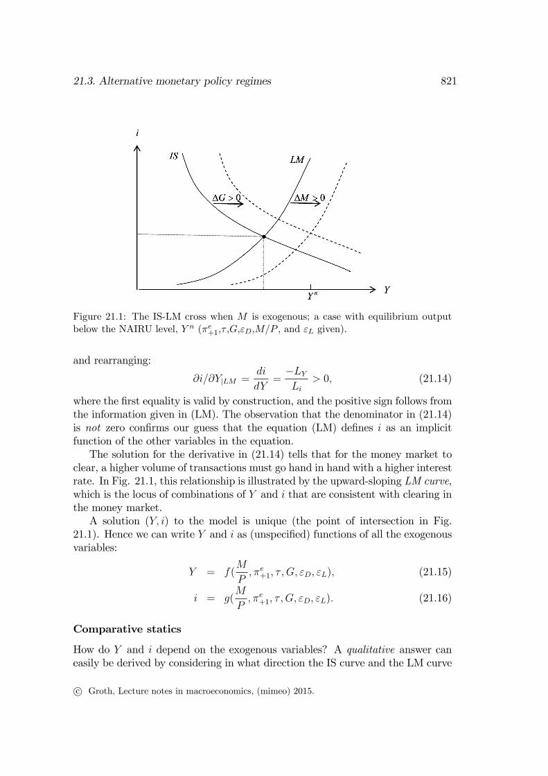
Figure 21.1: The IS-LM cross when M is exogenous; a case with equilibrium outputbelow the NAIRU level, Y n (πe+1,τ ,G,εD,M/P , and εL given).

and rearranging:

∂i/∂Y|LM =di

dY=−LYLi

> 0, (21.14)

where the first equality is valid by construction, and the positive sign follows fromthe information given in (LM). The observation that the denominator in (21.14)is not zero confirms our guess that the equation (LM) defines i as an implicitfunction of the other variables in the equation.The solution for the derivative in (21.14) tells that for the money market to

clear, a higher volume of transactions must go hand in hand with a higher interestrate. In Fig. 21.1, this relationship is illustrated by the upward-sloping LM curve,which is the locus of combinations of Y and i that are consistent with clearing inthe money market.A solution (Y, i) to the model is unique (the point of intersection in Fig.

21.1). Hence we can write Y and i as (unspecified) functions of all the exogenousvariables:

Y = f(M

P, πe+1, τ , G, εD, εL), (21.15)

i = g(M

P, πe+1, τ , G, εD, εL). (21.16)

Comparative statics

How do Y and i depend on the exogenous variables? A qualitative answer caneasily be derived by considering in what direction the IS curve and the LM curve



shift in response to a change in an exogenous variable. With minimal training,the directions of these shifts can be directly read off the information given in (IS)and (LM) equations. Alternatively one can use the total differentials (21.17) and(21.18) below also for this purpose.A quantitative answer is based on the standard comparative statics method.

Starting afresh with the (IS) - (LM) equation system, we guess that the systemdefines (determines) Y and i as implicit functions, f and g, of the other variables,as in (21.15) and (21.16). The aim is to find formulas for the partial derivatives ofthese implicit functions, evaluated at an equilibrium point (Y, i), a point satisfying(IS) and (LM). We first calculate the total differential on both sides of (IS):

dY = DY dY +Dre(di− dπe+1) +Dτdτ + dG+ dεD. (21.17)

Next we calculate the total differential on both sides of (LM):

d(M

P) = LY dY + Lidi+ dεL. (21.18)

We interpret these two equations as a new equation system with two new en-dogenous variables, the differentials dY and di. The changes, dπe+1, dG, dτ , dεD,d(M/P ), and dεL, in the exogenous variables are our new exogenous variables.The coeffi cients, DY , Dre , etc., to these endogenous and exogenous variables inthe two equations are derivatives evaluated at the equilibrium point (Y, i). Likethe original equation system (IS) - (LM), the new system is simultaneous (notrecursive).The key point is that the new system is linear. The further procedure is the

following. First rearrange (21.17) and (21.18) so that dY and di appear on theleft-hand side and the differentials of the exogenous variables on the right-handside of each equation:

(1−DY )dY −Dredi = −Dredπe+1 +Dτdτ + dG+ dεD, (21.19)

LY dY + Lidi = dM

P− dεL. (21.20)

Next, calculate the determinant, ∆, of the coeffi cient matrix on the left-hand sideof the system:

∆ =

∣∣∣∣ 1−DY −Dre

LY Li

∣∣∣∣ = (1−DY )Li +DreLY < 0, (21.21)

where the negative sign follows from qualitative information about the functionsD and L given in (IS) and (LM), respectively. The observation that the determi-nant is not zero confirms our guess that the (IS) - (LM) system defines Y and ias implicit functions of the other variables.



Now apply Cramer’s rule5 to the linear system (21.19) - (21.20) to determinedY and di:

dY =

∣∣∣∣ −Dredπe+1 +Dτdτ + dG+ dεD −Dre

dMP− dεL Li

∣∣∣∣∆

=Li(−Dredπ

e+1 +Dτdτ + dG+ dεD) +Dre(d

MP− dεL)

∆, (21.22)

and

di =

∣∣∣∣ 1−DY −Dredπe+1 +Dτdτ + dG+ dεD

LY dMP− dεL

∣∣∣∣∆

=(1−DY )(dM

P− dεL)− LY (−Dredπ

e+1 +Dτdτ + dG+ dεD)

∆.(21.23)

The partial derivatives of f and g, respectively, w.r.t. the exogenous variablescan be directly read off these two formulas.Suppose we are interested in the effect on Y and i of a change in the real

money supply, M/P. By setting dπe+1 = dτ = dG = dεD = dεL = 0 in (21.22)and (21.23) and rearranging, we get

∂Y

∂(MP

)= fM/P =

dY

d(MP

)=

Dr

(1−DY )Li +DreLY> 0,

∂i

∂(MP

)= gM/P =

di

d(MP

)=

1−DY

(1−DY )Li +DreLY< 0,

where the signs are due to (21.6), 21.7, and (21.21). Such partial derivatives of theendogenous variables w.r.t. an exogenous variable, evaluated at the equilibriumpoint, are known as multipliers. The approximative short-run effect on Y of agiven small increase dM in M is calculated as dY = (∂Y/∂(M

P))dM/P, where we

see the role of the partial derivative w.r.t. M/P as a multiplier on the increasein the exogenous variable, M/P .6

5See Math Tools.6Instead of using Cramer’s rule, in the present case we could just substitute di, as determined

from (21.18), into (21.17) and then find dY from this equation. In the next step, this solutionfor dY can be inserted into (21.18), which then gives the solution for di. However, if Li werea function that could take the value nil, this procedure might invite a temptation to rule thisout by assumption. That would imply an unnecessary reduction of the domain of f(·) and g(·).The only truly necessary assumption is that ∆ 6= 0 and that is automatically satisfied in thepresent problem.



The intuitive interpretation of the signs of these multipliers is the following.The central bank increases the money supply through an open market purchase ofbonds held by the private sector. In practice it is usually short-term governmentbonds (“treasury bills”) that the central bank buys when it wants to increasethe money supply (decrease the short-term interest rate). Immediately after thepurchase, the supply of money is higher than before and the supply of bondsavailable to the public is lower. At the initial interest rate there is now excesssupply of money and excess demand for bonds. But the attempt of agents toget rid of their excess cash in exchange for more bonds can not succeed in theaggregate because the supplies of bonds and money are given. Instead, whathappens is that the price of bonds goes up, that is, the interest rate goes down,cf. (21.10), until the available supplies of money and bonds are willingly held bythe agents. Money is therefore not neutral.To find the output multiplier w.r.t. government spending on goods and ser-

vices, or what is known as the spending multiplier, in (21.22) we set d(M/P )= dπe+1 = dτ = dεD = dεL = 0 and rearrange to get

∂Y

∂G= fG =

dY

dG=

Li(1−DY )Li +DreLY

=1

1−DY +DreLY /Li. (21.24)

Under the assumed monetary policy we thus have 0 < ∂Y/∂G < 1/(1 − DY ).The difference, 1/(1−DY ) −∂Y/∂G, is due to the financial crowding-out effect,represented by the term DreLY /Li > 0 in (21.24). Owing to the fixed moneystock, the expansionary effect of a rise in G is partly offset by a rise in theinterest rate induced by the increased money demand resulting from the “initialrise”in economic activity. If money demand is not sensitive to the interest rate7

(as the monetarists claimed), the financial crowding-out is large and the spendingmultiplier low in this policy regime.Another “moderator”comes from the marginal net tax rate, T ′(Y ) ∈ (0, 1),

which by reducing the private sector’s marginal propensity to spend, DY in (21.6),acts as an automatic stabilizer. When aggregate output (economic activity) rises,disposable income rises less, partly because of higher taxation, partly because oflower aggregate transfers, for example unemployment compensation.8

Shifts in the values of the exogenous variables, εD and εL, may be interpretedas shocks (disturbances) coming from a variety of unspecified events. A positivedemand shock, dεD > 0, may be due to an upward shift in households’and firms’

7This is the case when |Li| is low, i.e., the LM curve steep.8Outside our static IS-LM model an additional issue is how current consumers repond to the

increased public debt in the wake of a not fully tax-financed temporary increase in G. Althoughthis takes us outside the static IS-LM model, we shall briefly comment on it towards the endof this chapter.



“confidence”. A negative demand shock may come from a “credit crunch”due toa financial crisis. A positive liquidity preference shock may reflect a sudden risein the perceived risk of default of bond liabilities.To see how demand shocks and liquidity preference shocks, respectively, affect

output under the given monetary policy, in the equation (21.22) we set dπe+1 = dτ= dG = dM

P= 0. When in addition we set, first, dεL = 0, and next dεD = 0, we

find the partial derivatives of Y w.r.t. εD and εL, respectively:

∂Y

∂εD= fεD =

dY

dεD=

Li(1−DY )Li +DreLY

=1

1−DY +DreLY /Li∂Y

∂εL= fεL =

dY

dεL=

−Dre

(1−DY )Li +DreLY< 0.

As expected, a positive demand shock is expansionary, while a positive liquiditypreference shock is contractionary because it raises the interest rate. Note that∂Y/∂εD = ∂Y/∂G (from (21.24)) in view of the way εD enters the IS equation.As now the method should be clear, we present the further results without

detailing. From (21.22) and (21.23), respectively, we calculate the output andinterest multipliers w.r.t. fiscal tightness to be

∂Y

∂τ=

LiDτ

(1−DY )Li +DreLY< 0,

∂i

∂τ=

−LYDτ

(1−DY )Li +DreLY< 0.

What do (21.22) and (21.23) imply regarding the effect of higher expected infla-tion on Y, i, and re, respectively? We find

∂Y

∂πe+1

= fπe+1=

−LiDre

(1−DY )Li +DreLY> 0,

∂i

∂πe+1

= gπe+1=

LYDre

(1−DY )Li +DreLY∈ (0, 1), (21.25)

∂re

∂πe+1

=∂(i− πe+1)

∂πe+1

= gπe+1− 1 =

−(1−DY )Li(1−DY )Li +DreLY

∈ (−1, 0).

A higher expected inflation rate thus leads to a less-than-one-to-one increase inthe nominal interest rate and thereby a smaller expected real interest rate. Onlyif money demand were independent of the nominal interest rate (Li = 0), as inthe quantity theory of money, would the nominal interest rate rise one—to-onewith πe+1 and the expected real interest rate thereby remain unaffected.Before proceeding, note that there is a reason that we have set up the IS

and LM equations in a general nonlinear form. We want the model to allow



Figure 21.2: A fixed interest rate implying equilibrium output close to the NAIRU level(i,πe+1, τ , G, and εD given).

for the empirical feature that the different multipliers generally depend on the“state of the business cycle”. The spending multiplier, for instance, tends tobe considerably larger in a slump − with plenty of idle resources − than in aboom. In dynamic extensions of the IS-LM model the length of the time intervalassociated with the higher G becomes important as does the time profile of theeffect on Y . In the present static version of the model it fits intuition best tointerpret the rise in G as referring to the “current”period only.

21.3.2 Fixed interest rate rule

Instead of targeting a certain level of the money stock, the central bank nowkeeps the nominal interest rate at a certain target level i > 0. The aim may beto have output unaffected by liquidity preference shocks. This monetary policyseems closer to what most central banks nowadays typically do. They announcea target for the nominal interest rate and then, through open-market operations,adjust the monetary base so that the target rate is realized.In this regime, i is an exogenous constant > 0, whileM and Y are endogenous.

Instead of the upward-sloping LM curve we get a horizontal line, the IR line inFig. 21.2 (“IR” for interest rate). The model is now recursive. Since M doesnot enter the equation (IS), Y is given by this equation independently of theequation (LM). Indeed, in view of DY 6= 0, the equation (IS) defines Y as an



implicit function, h, of the other variables in the equation, i.e.,

Y = h(re, τ , G, εD) = h(i− πe+1, τ , G, εD). (21.26)

Comparative statics

The partial derivatives of the function h can be directly read off equation (21.17).We find

∂Y

∂i= hre =

Dre

1−DY

< 0,

∂Y

∂πe+1

= −hre = − Dre

1−DY

> 0,

∂Y

∂τ= hτ =

Dτ

1−DY

< Dτ < 0, (21.27)

∂Y

∂G=

∂Y

∂εD=

1

1−DY

> 1,

∂Y

∂εL= 0.

The observation that the denominator, 1 − DY , is not zero confirms our guessthat the equation (IS) defines Y as an implicit function of the other variables inthe equation.The derivative w.r.t. a liquidity preference shock, εL, in the last line of (21.27)

reflects the principle that a multiplier w.r.t. an exogenous variable not enteringthe equation(s) determining the endogenous variable directly or indirectly (seebelow) is nil. In the present case this means that, with a fixed interest rule,a liquidity preference shock has no effect on equilibrium output. The shock isimmediately counteracted by a change in the money stock in the same directionso that the interest rate remains unchanged. Thus, the liquidity preference shockis “cushioned”by this monetary policy.On the other hand, a shock to output demand has a larger effect on output

than in the case where the money stock is kept constant (compare (21.27) to(21.24)). This is because keeping the money stock constant allows a dampeningrise in the interest rate to take place. But with a constant interest rate thisfinancial crowding-out effect does not occur.One is tempted to draw the conclusion (from Poole, 1970):

• a money stock rule is preferable (in the sense of implying less volatility) ifmost shocks are output demand shocks, while

• a fixed interest rate rule is preferable if most shocks are liquidity preferenceshocks.



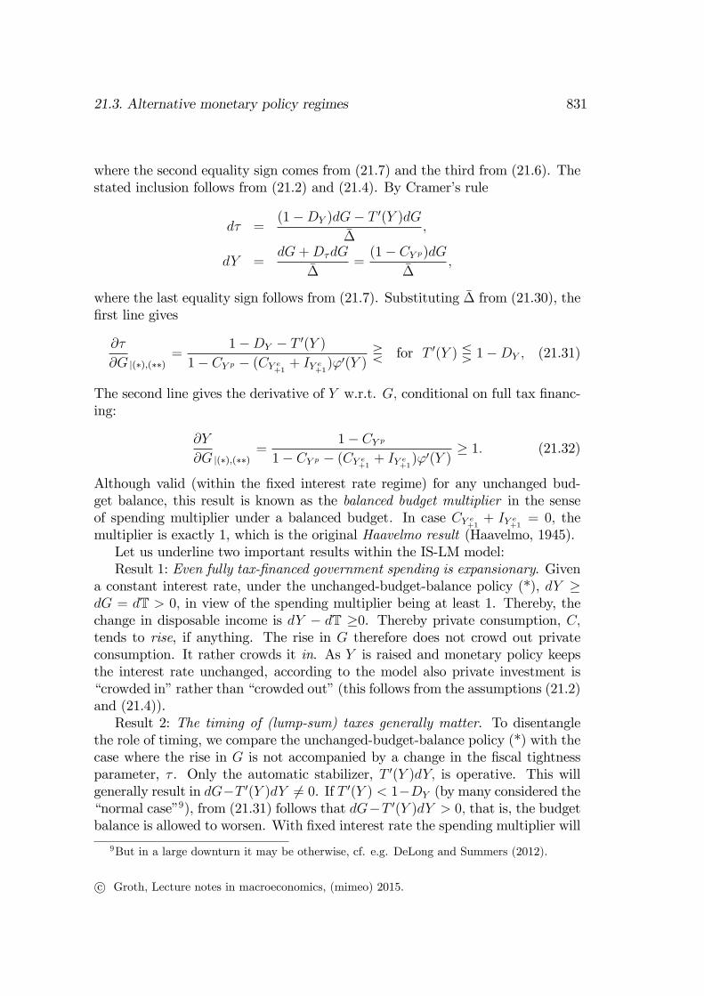
Figure 21.3: Given a fixed interest rate, a “Keynesian cross” diagram is suffi cient todisplay the equilibrium output level (i, πe+1, τ , G, and εD given).

This should be accepted with caution, however, since a static model is not asecure guide for policy rules.If we are interested also in the required changes in the money stock, we rewrite

(LM) as

M = P · (L(Y, i) + εL). (LM’)

Here, i is exogenous and Y should be seen as already determined from (IS) in-dependently of (LM’), that is, as given by (21.26). In this context we consider(LM’) as an equation determiningM as an implicit function of the other variablesin the equation. To find the partial derivatives of this function, we take the totaldifferential on both sides of (LM’):

dM = P (LY dY + Lidi+ dεL) + (L(Y, i) + εL)dP, (21.28)

where dY can be seen as already determined from (21.17) through (21.27), inde-pendently of (21.18). For instance, the approximate change in the money stockrequired for a rise in i of size di > 0 to materialize can, by (21.28), be written

∆M ≈ dM = PLY dY + PLidi = PLY hredi+ PLidi = PLYDre

1−DY

+ PLidi,

where the first term after the second equality sign is based on using the chain



rule in (LM’). The multiplier of the money stock w.r.t. i is

∂M

∂i |(LM ′)=

∂M

∂Y |(LM ′)· ∂Y∂i |(21.26)

+∂M

∂i |(LM ′)=dM

dY |21.28hre +

dM

di |21.28

= PLYDre

1−DY

+ PLi < 0,

where the first term after the last equality sign represents a negative indirecteffect on the money stock of the rise in the target and the second term a negativedirect effect. The direct effect indicates the fall in money stock needed to inducea rise in the interest rate of size di for a fixed output level. But also the outputlevel will be affected by the rise in the interest rate since this rise reduces outputdemand. Through this indirect channel the transactions-motivated demand formoney is reduced, and to match this a further fall in the money stock is required.This is the indirect effect.The multipliers for the money stock w.r.t. the other exogenous variables are

found in a similar way from (21.28) and (21.27), again using the chain rule whereappropriate. Let us first consider the multiplier w.r.t. the exogenous variablesentering (IS) and thereby (21.26). We get :

∂M

∂πe+1

= PLY∂Y

∂πe+1 |(21.26)

= PLy · (−hre) = −PLYDre

1−DY

> 0,

∂M

∂τ= PLY

∂Y

∂τ |(21.26)= PLy · hτ = PLY

Dτ

1−DY

< 0,

∂M

∂G=

∂M

∂εD= PLY

∂Y

∂G |(21.26)= PLy · hG = PLY

1

1−DY

> 0,

where the inserted partial derives of h come from (21.27).We see that higher expected inflation implies that the money stock required to

maintain a given interest rate is higher. The reason is that for given i, a higher πe+1

means lower expected real interest rate, hence higher output demand and higheroutput. Hereby the transactions-motivated demand for money is increased. Ahigher money stock is thus needed to hinder a rise in the nominal interest rateabove target.Finally, as εL and P do not enter (IS) and thereby not (21.26), the multipliers

of M w.r.t. these two variables are determined directly by (LM’), keeping Y andi constant. We get

∂M

∂εL= P > 0,

∂M

∂P= L(Y, i) + εL =

M

P> 0.

The “Keynesian cross” Since for a fixed interest rate there is no financialcrowding-out, the production outcome can also be illustrated by a standard 45◦

“Keynesian cross”diagram as in Fig. 21.3.



The spending multiplier under full tax financing

The spending multiplier in the last line of (21.27) is conditional on the fixedinterest rate policy and constancy of the “fiscal tightness”, τ . Although therewill be an automatic rise in net tax revenue via T ′(Y ) > 0, unless increasedgovernment spending is fully self-financing (which it will be only if T ′(Y ) ≥1 −DY , as we will see in a moment), the result is dT < dG. This amounts to alarger budget deficit than otherwise and thereby increased public debt and highertaxes in the future. In Section 21.4 below we assess the possible feedback effectsof this on the spending multiplier (effects that are ignored by the static IS-LMmodel).In the present section we will consider the alternative case, a useful bench-

mark, where the increase in G is accompanied by an adjustment of the fiscaltightness parameter, τ , so as to ensure dT = dG, thereby leaving the budgetbalance unchanged, it be negative, positive, or nil. The net tax revenue is

T = τ + T (Y ), 0 ≤ T ′ < 1, (21.29)

cf. Section 21.1. We impose the requirement that the primary budget deficit,G − T, remains equal to some constant k in spite of the change in G.This givesthe equation

G− τ − T (Y ) = k, (*)

where both τ and Y are endogenous. We have a second equation where these twovariables enter, namely the (IS) equation with i exogenous:

Y = D(Y, i− πe+1, τ) +G, (**)

ignoring the shift term εD. The equation system (*) - (**) thus determines thepair τ and Y as implicit functions of the remaining variables, all of which areexogenous.Taking differentials w.r.t. Y, τ , and G on both sides of (*) and (**) gives,

after ordering, the linear equation system in dτ and dY :

dτ + T ′(Y )dY = dG

−Dτdτ + (1−DY )dY = dG.

The determinant of the coeffi cient matrix on the left-hand side of this system is

∆ = 1−DY +DτT′(Y ) = 1−DY − CY pT ′(Y )

= 1−[CY p(1− T ′(Y )) + (CY e+1

+ IY e+1)ϕ′(Y )

]− CY pT ′(Y )

= 1− CY p − (CY e+1+ IY e+1

)ϕ′(Y ) ∈ (0, 1), (21.30)



where the second equality sign comes from (21.7) and the third from (21.6). Thestated inclusion follows from (21.2) and (21.4). By Cramer’s rule

dτ =(1−DY )dG− T ′(Y )dG

∆,

dY =dG+DτdG

∆=

(1− CY p)dG∆

,

where the last equality sign follows from (21.7). Substituting ∆ from (21.30), thefirst line gives

∂τ

∂G |(∗),(∗∗)=

1−DY − T ′(Y )

1− CY p − (CY e+1+ IY e+1

)ϕ′(Y )R for T ′(Y ) Q 1−DY , (21.31)

The second line gives the derivative of Y w.r.t. G, conditional on full tax financ-ing:

∂Y

∂G |(∗),(∗∗)=

1− CY p1− CY p − (CY e+1

+ IY e+1)ϕ′(Y )

≥ 1. (21.32)

Although valid (within the fixed interest rate regime) for any unchanged bud-get balance, this result is known as the balanced budget multiplier in the senseof spending multiplier under a balanced budget. In case CY e+1

+ IY e+1= 0, the

multiplier is exactly 1, which is the original Haavelmo result (Haavelmo, 1945).Let us underline two important results within the IS-LM model:Result 1: Even fully tax-financed government spending is expansionary. Given

a constant interest rate, under the unchanged-budget-balance policy (*), dY ≥dG = dT > 0, in view of the spending multiplier being at least 1. Thereby, thechange in disposable income is dY − dT ≥0. Thereby private consumption, C,tends to rise, if anything. The rise in G therefore does not crowd out privateconsumption. It rather crowds it in. As Y is raised and monetary policy keepsthe interest rate unchanged, according to the model also private investment is“crowded in”rather than “crowded out”(this follows from the assumptions (21.2)and (21.4)).Result 2: The timing of (lump-sum) taxes generally matter. To disentangle

the role of timing, we compare the unchanged-budget-balance policy (*) with thecase where the rise in G is not accompanied by a change in the fiscal tightnessparameter, τ . Only the automatic stabilizer, T ′(Y )dY, is operative. This willgenerally result in dG−T ′(Y )dY 6= 0. If T ′(Y ) < 1−DY (by many considered the“normal case”9), from (21.31) follows that dG−T ′(Y )dY > 0, that is, the budgetbalance is allowed to worsen. With fixed interest rate the spending multiplier will

9But in a large downturn it may be otherwise, cf. e.g. DeLong and Summers (2012).



be 1/(1−DY ), cf. (21.27), and exceed that under an unchanged budget balance,given in (21.32).10 So in the considered case, postponing the taxation needed toprovide the ultimate financing of the rise in G makes this rise more expansionary.The timing of taxes matter.In Section 21.4 we briefly discuss what happens to these two results if we

imagine that the household sector consists of a fixed number of utility-maximizinginfinitely-lived households.

The paradox of thrift

Another proposition of Keynesian theory is known as the paradox of thrift. Con-sider the following special case of the IS equation:

Y = C + I +G = c0 + c1(Y − T) + C(i− πe+1) + c2Y + I(i− πe+1) +G, (21.33)

where c0, c1, and c2 are given constants satisfying

c0 > 0, 0 < c1 ≤ c1 + c2 < 1, (21.34)

and C (·) and I (·) are decreasing functions of the expected real interest rate,i − πe+1. We have excluded the demand shift parameter εD and linearized theincome-dependent parts of the consumption and investment functions. We takeG, πe+1, and i as exogenous (fixed interest rate rule).The paradox of thrift comes out most clear-cut if we ignore the public sector.

No public sector: G = T = 0. In this case equilibrium output is

Y =c0 + C(i− πe+1) + I(i− πe+1)

1− c1 − c2

.

Suppose that all households for some reason decide to save more at any levelof income so that c0 is decreased. What happens to aggregate private saving Sp?We have

Sp = Y − C = I = c2Y + I(i− πe+1), (21.35)

by (21.33) with G = T = 0. Hence,

∂Sp

∂c0

= c2∂Y

∂c0

=c2

1− c1 − c2

≥ 0,

from (21.27). Considering a reduction of c0, i.e., ∆c0 < 0, the resulting changein Sp is thus

∆Sp =∂Sp

∂c0

∆c0 =c2

1− c1 − c2

∆c0 ≤ 0.

10Indeed, 1/(1−DY ) R (1− CY P )/(1−DY − CY P T ′(Y )) if T ′(Y ) < 1−DY , respectively.



The attempt to save more thus defeats itself. What happens is that incomedecreases by an amount such that saving is either unchanged or even reduced.More precisely, if the income coeffi cient in the investment function, c2, is nil, weget ∆Sp = 0 because aggregate investment remains unchanged and income isreduced exactly as much as consumption, leaving saving unchanged. If c2 > 0,we get ∆Sp < 0 because income is reduced more than consumption since alsoinvestment is reduced when income is reduced. In this case the attempt to savemore is directly counterproductive and leads to less aggregate saving.The background to these results is that when aggregate output and income

is demand-determined, the decreased propensity to consume lowers aggregatedemand, thereby reducing production and income. The resulting lower incomebrings aggregate consumption further down through the Kahn-Keynes multiplierprocess (see below). While consumption is reduced, there is nothing in the sit-uation to stimulate aggregate investment (at least not as long as the centralbank maintains an unchanged interest rate). Thereby aggregate saving can notrise, since in a closed economy aggregate saving and aggregate investment arein equilibrium just two sides of the same thing as testified by national incomeaccounting, cf. (21.35).This story is known as the paradox of thrift. It is an example of a fallacy

of composition, a term used by philosophers to denote the error of concludingfrom what is locally valid to what is globally valid. Such inference overlooks thepossibility that when many agents act at the same time, the conditions framingeach agent’s actions are affected. As Keynes put it:

. . . although the amount of his own saving is unlikely to have anysignificant influence on his own income, the reactions of the amountof his consumption on the incomes of others makes it impossible forall individuals simultaneously to save any given sums. Every suchattempt to save more by reducing consumption will so affect incomesthat the attempt necessarily defeats itself (Keynes 1936, p. 84).

With public sector We return to (21.33) with G > 0 and T > 0. The essenceof the paradox of thrift remains but it may be partly blurred by the tendency ofthe government budget deficit to rise when private consumption, and thereforeaggregate income, is reduced.Consider first the case where public dissaving does not emerge. This is the

case where the government budget is always balanced. Then, net tax revenue isT = G, and private saving is

Sp ≡ Y − T−C = Y −G− C = I = c2Y + I(i− πe+1),



by (21.33). So in this case the paradox of thrift comes out in the same strongform as above.Consider instead the more realistic case where alternating budget deficits and

surpluses are allowed to arise as a result of the net tax revenue following the rule

T = τ + τ 1Y, 0 < τ 1 < 1. (21.36)

Equilibrium output now is

Y =c0 − c1τ + C(i− πe+1) + I(i− πe+1) +G

1− c1(1− τ 1)− c2

, (21.37)

so that∂Y

∂c0

=1

1− c1(1− τ 1)− c2

> 1, (21.38)

the inequality being due to (21.34) and (21.36). Private saving is

Sp = Y − T− C = I − (T−G) = I − Sg = I +G− (τ + τ 1Y )

= c2Y + I(i− πe+1) +G− (τ + τ 1Y ),

where the second equality comes from (21.33) and the fourth from the taxationrule (21.36). We see that.....(continuation not yet available)

Adjustment: the Kahn-Keynes multiplier process (no text available)

21.3.3 Counter-cyclical interest rate rule

Assuming a fixed interest rate rule may fit the very short run well. If we think of atime interval of a year’s length or more, we may imagine a counter-cyclical interestrate rule aiming at dampening fluctuations in aggregate economic activity. Sucha policy may take the form

i = i0 + i1Y, i1 > 0, (21.39)

where i0 and i1 are policy parameters. The present version of the IS-LM modeldoes not rule out that the parameter i0 can be negative. But in case i0 < 0, atleast i0 is not so small that even under “normal circumstances”, the zero lowerbound for i can become operative. The term “counter-cyclical” refers to theattempt to stabilize output by raising i when output goes up and reducing iwhen output goes down.11

11The label “counter-cyclical” should not be confused with what is in the terminology ofbusiness cycle econometrics named “counter-cyclical”behavior. In this terminology a variableis characterized as “pro-”or “counter-cyclical”depending on whether its correlation with ag-gregate output is positive or negative, respectively. So (21.39) would in this language exemplify“pro-cyclical”behavior.



If the LM curve in Fig. 21.1 is made linear and its label changed into IRR(for Interest Rate Rule), that figure covers the counter-cyclical interest rate rule(21.39). Instead of a LM curve (which requires a fixed M), we have an upwardsloping IRR curve. Both i and M are here endogenous. The fixed interest raterule from the previous section is a limiting case of this rule, namely the casei1 = 0. By having i1 > 0, the counter-cyclical interest rate rule yields qualitativeeffects more in line with those of a money stock rule. If i1 > ∂i/∂Y|LM from(21.14), the stabilizing response of i to a decrease in Y is stronger than underthe money stock rule.

Comparative statics

Inserting (21.39) into (IS) gives

Y = D(Y, i0 + i1Y − πe+1, τ) +G+ εD.

By taking the total differential on both sides we find

∂Y

∂G=

∂Y

∂εD=

1

1−DY −Drei1∈ (0,

1

1−DY

),

∂Y

∂i1=

DreY

1−DY −Drei1< 0,

∂Y

∂πe+1

= − Dre

1−DY −Drei1> 0,

∂Y

∂εL= 0.

We see that all multipliers become become close to 0, if the reaction coeffi cient i1is large enough. In particular, undesired fluctuations due to demand shocks aredamped this way.The corresponding changes in i are given as ∂i/∂x = i1∂Y/∂x for x= G, εD, i1, π

e+1,

and εL, respectively. From (21.28) we find the corresponding changes in M as∂M/∂x = P (LY + i1Li)∂Y/∂x for x = G, εD, i1, and πe+1; finally, from (21.28) wehave again ∂M/∂εL = P > 0.

21.3.4 Further aspects

The loanable funds theory of the interest rate

As we have seen, two Keynesian tenets are that involuntary unemployment canbe a state of rest and that an increased propensity to save makes things worse.Several of Keynes’contemporaries (for instance NAME, YEAR) objected that



the interest rate would adjust so as to bring the demand for new loans by users(primarily home and business investors).in line with an increased supply of newloans by financial savers. This is known as the “loanable funds theory of theinterest rate”according to which the interest rate is determined by “the supplyand demand for saving”. The pre-Keynesian version of this theory does not takeinto account that aggregate saving depends not only on the interest rate, but alsoon aggregate income (the same could be said about investment but this is of nohelp for the pre-Keynesian version).To clarify the issue, we consider the simple case where C = C(Y, re) and I

= I(re), 0 < CY < 1, Cre < 0, Ire < 0, re = i − πe+1 and where governmentspending and taxation are ignored. Let S denote aggregate saving. Then in ourclosed economy, S = Y − C = Y − C(Y, re) ≡ S(Y, re), SY = 1 − CY > 0,Sre = −Cre > 0. Equilibrium in the output market requires Y = C(Y, re) + I(re).By subtracting C(Y, re) on both sides and inserting re = i− πe+1, we get

S(Y, i− πe+1) = I(i− πe+1), (21.40)

which may be interpreted as supply of saving being equilibrated with demand forsaving. Conditional on a given income level, Y , we could draw an upward-slopingsupply curve and a downward-sloping demand curve in the (S, i) plane for givenπe+1. But this would not determine i since the position of the supply curve willdepend on the endogenous variable, Y. An extra equation is needed. This is whatthe money market equilibrium condition, M/P = L(Y, i) delivers, combined withexogeneity ofM, P and πe. In the Keynesian version of the loanable funds theoryof the interest rate there are thus two endogenous variables, i and Y, and twoequations, (21.40) and M/P = L(Y, i).If we want to illustrate the solution graphically, we can use the standard IS-

LM diagram from Fig. 21.1. This is because the equation (21.40) in the (Y, i)plane is nothing but the standard IS curve. Indeed, by adding consumption onboth sides of the equation, we get Y = C(Y, i−πe+1) +I(i−πe+1), the standard ISequation. And whether we combine the LM equation with this or with (21.40),the solution for the pair (Y, i) will be the same.

A liquidity trap

We return to the general IS-LM model,

Y = D(Y, i− πe+1, τ) +G+ εD, (IS)M

P= L(Y, i) + εL, (LM)

where M is again exogenous and Y and i endogenous. Suppose a large adversedemand shock εD < 0 takes place. This shock could be due to a bursting housing



Figure 21.4: A situation where the given IS curve is such that no non-negative nominalinterest rate can generate full employment (πe+1, τ , G, εD, M/P , and εL given). Thevalue of Y where the IS curve crosses the abscissas axis is dented Y0.

price bubble making creditors worried and demanding that debtors deleverage.This amounts to decreased consumption and investment and as a consequence,the IS curve may be moved so much leftward in the IS-LM diagram that whateverthe money stock, output will end up smaller than the full-employment level, Y n.Then the economy is in a liquidity trap: “conventional”monetary policy is notable to move output back to full employment. By “conventional”monetary policyis meant a policy where the central bank buys bonds in the open market withthe aim of reducing the short-term nominal interest rate and thereby stimulateaggregate demand . The situation resembles a “trap”in the sense that when thecentral bank strives to stimulate aggregate demand by lowering the interest ratethrough open market operations, it is like attempting to fill a leaking bucket withwater. The phenomenon is illustrated in Fig. 21.4.

The crux of the matter is that the nominal interest rate has the lower bound,0, known as the zero lower bound. An increase in M can not bring i below 0.Agents would prefer holding cash at zero interest rather than short-term bondsat negative interest. That is, equilibrium in the asset markets is then consistentwith the “=”in the LM equation being replaced by “≥”.Suppose that expected inflation is very low, say nil. Then the (expected) real

interest rate can not be brought below zero. The real interest rate required forfull employment is negative, however, given the IS curve in Fig. 21.4. For thegiven πe, to solve the demand problem expansionary fiscal policy moving the IS



curve rightward is called for. Coordinated fiscal and monetary policy with theaim of raising πe may also be a way out.

When an economy is at the zero lower bound, the government spending mul-tiplier tends to be relatively large for two reasons. The first reason is the moretrivial one that being in a liquidity trap is a symptom of a serious deficient aggre-gate demand problem and low capacity utilization so that there is no hindrancefor fast expansion of production. The second reason is that there will be no fi-nancial crowding-out effect of a fiscal stimulus as long as the central bank aimsat an interest rate as low as possible. (REFER to lit.)

Note that the economy can be in a liquidity trap, as we have defined it,before the zero lower bound on the nominal interest rate has been reached. Fig.21.4 illustrates such a case. In spite of the current nominal interest rate beingabove zero, conventional monetary policy is not able to move output back to fullemployment. Conventional monetary policy can move the LM curve to the right,but the point of intersection with the IS curve can not be moved to the rightof Y0. An alternative − and more common − definition is simply to identify aliquidity trap with a situation in which the short-term nominal interest rate iszero.

Keynes (1936, p. 207) was the first to consider the possibility of a liquiditytrap. After the second world war the issue appeared in textbooks, but not inpractice, and so it gradually was given less and less attention. Almost at thesame time as the textbooks had stopped mentioning it, it turned up in reality,first in Japan from the middle of the 1990, then in several countries, includingUSA, in the wake of the Great Recession. It became a problem of urgent practicalimportance and lead to suggestions for non-conventional monetary policies as wellas more emphasis on expansionary fiscal policy, aspects to which we return laterin this book.

A proviso concerning the exact character of the zero lower bound on the inter-est rate should be added. The zero bound should only be interpreted as exactly0.0 if storage, administration, and safety cost are negligible, and − in an openeconomy − if there is no chance of a sudden appreciation of the currency in whichthe government debt is denominated. In the wake of the European debt crisis2010-14, government bonds of some European countries (e.g., Germany, Finland,Switzerland, Denmark, and the Netherlands) were sold at slightly negative yields.

–

Unfinished:

Some empirics about spending multipliers and their dependence on the stateof the economy.


21.4. Some robustness checks 839

21.4 Some robustness checks

21.4.1 Presence of an interest rate spread (banks’lendingrate = i+ ω > i).

(currently no text)

21.4.2 What if households are infinitely-lived?

Here we shall reconsider Result 1 and Result 2 from Section 21.3.2. They were:Result 1: Even fully tax-financed government spending is expansionary.Result 2: The timing of (lump-sum) taxes generally matter.We ask whether these two results are likely to still hold in some form if we

imagine that the household sector consists of a fixed number of utility-maximizinginfinitely-lived households. The assumption that involuntary unemployment andabundant capacity are present is maintained.Concerning Result 1 the answer is yes in the sense that the spending multiplier

under a balanced budget will remain positive, albeit not necessarily ≥ 1. Thereason is that although under a balanced budget the households face a temporaryrise in taxes, dT, equal to the temporary rise in spending, dG, they will reducetheir current consumption by less than dT, if at all. This is because they wantto smooth consumption. If they at all have to reduce their total consumption,they will spread this reduction out over all future periods so that the presentvalue of the total reduction is suffi cient to cover the rise in taxes. Thereby,−dC < dG so that there is necessarily an “initial”stimulus to aggregate demandequal to dG−dC > 0.Owing to unemployment and abundant production capacity,there need not be any crowding out of investment and so aggregate demand,output, and employment will be higher in this “first round”than without the risein G. This means that current before-tax incomes increase and this stimulatesprivate consumption and, therefore, production in the “second round”. Andso on through the “multiplier process”. In the end private consumption in thecurrent period need not at all fall and may even rise. So even with infinitely-livedhouseholds, the rise in G is expansionary under the stated circumstances.Concerning Result 2 the answer depends on whether the credit market is

perfect or not. With a perfect credit market current consumption of the infinitely-lived households will not depend on the timing of the extra taxes that are neededto finance dG. Whether the tax rise occurs now or later is irrelevant, as long asthe present value of the tax rise is the same for the individual household. Sothe spending multiplier will be the same in the two situations. In this case, inspite of the rise in G being expansionary, there is Ricardian equivalence in thesense that for a given time path of government expenditures, the time path of



(lump-sum) taxes does not matter for aggregate private consumption (whetherthe taxes are lump-sum or distortionary is in fact not so important in the presentcontext where production and employment are demand-determined rather thansupply-determined).If the credit market is imperfect, however, in a heterogeneous population some

of the infinitely-lived households, the less patient, say, may be currently creditconstrained. The timing of the extra taxes then does matter and Ricardian equiv-alence is absent. Indeed, the lower current taxes associated with a budget deficitloosens the limit to current consumption of the credit-constrained households.Their consumption demand is thereby stimulated. Aggregate demand and there-fore output and employment are thus raised. Through the automatic stabilizersthe budget deficit hereby becomes smaller than otherwise. This means that thefuture extra tax burden becomes lower for everybody, including the householdsthat are not currently credit-constrained. So also their current consumption isstimulated, and aggregate demand is raised further. We conclude that in spite ofhouseholds being infinitely-lived, when credit markets are imperfect, for a givenrise in government spending, the spending multiplier is likely to be larger underdeficit financing than under balanced budget financing. So even Result 2 seemsrelatively robust.

21.5 Concluding remarks

The distinguishing feature of the IS-LM model compared with classical and new-classical theory is the treatment of the general price level for goods and servicesas given in the short run, that is, as a state variable of the system, hence verydifferent from an asset price. The IS-LM model is not about why it is so (thetwo previous chapters suggested some answers to that question), but about theconsequences for how the interaction between goods and asset markets works out.There are two different assets, money and an interest-bearing asset in the formof bonds, where money is held because of its liquidity services while as a store ofvalue money is generally dominated by bonds.Traditionally, the IS-LM model has been seen as only one building block of a

more involved aggregate supply-aggregate demand (AS-AD) framework of manymacroeconomic textbooks. In that framework the IS-LM model describes justthe demand side of a model where the level of nominal wages is an exogenousconstant in the short run, but the price level adjusts in response to shifts inaggregate demand for fixed money stock.In this chapter we have interpreted the IS-LM model another way, namely

as an independent short-run model in its own right, based on the approximationthat both nominal wages and prices are set “in advance”by agents operating in


21.6. Literature notes 841

imperfectly competitive markets and being hesitant regarding frequent or largeprice changes. The traditional AS-AD version of the Keynesian framework blursthe distinction between short-run equilibrium and a sequence of such equilibria.In a sequence of short-run equilibria some kind of Phillips curve, a dynamicrelation, is operative rather than an upward-sloping AS curve in the (Y, P ) plane(a static relation).12

Given the pre-set wages and prices, in every short period output is demand-determined. Likewise, but behind the scene, also employment is demand-determined.Not prices on goods and services, but quantities are the equilibrating factors.This is the polar opposite of Walrasian microeconomics and neoclassical long-runtheory, cf. Part II-IV of this book, where output and employment are treatedas supply-determined − with absolute and relative prices as the equilibratingfactors.A striking implication of this role switch is the paradox of thrift which is

Keynes’favorite example of a fallacy of composition. As Keynes put it:

. . . although the amount of his own saving is unlikely to have anysignificant influence on his own income, the reactions of the amountof his consumption on the incomes of others makes it impossible forall individuals simultaneously to save any given sums. Every suchattempt to save more by reducing consumption will so affect incomesthat the attempt necessarily defeats itself (Keynes 1936, p. 84).

Empirically the IS-LM model, in the interpretation given here but extendedwith an expectation-augmented Phillips curve, does a quite good job (see Gali,1992, and Rudebusch and Svensson, 1998). And for instance the surveys inthe Handbook of Macroeconomics (1999) and Handbook of Monetary Economics(201?) support the view that under “normal circumstances”, the empirics saythat the level of production and employment is significantly sensitive to fiscaland monetary policy.

21.6 Literature notes

The IS-LM model as presented here is essentially based on the attempt by Hicks(1937) to summarize the analytical content of Keynes’General Theory of Em-

12If one insists on something related to AS-AD, one could interpret this chapter’s model asimposing a horizontal AS curve in the output-price plane. But that’s it. No AD curve in thisplane appears in the model. The only place an AD curve appears is in the output-interest planein the form of an IS curve. When it comes to the study of sequences of short-run equilibria(Chapter 22), a medium-term AD curve in the output-inflation plane will arise.



ployment, Interest and Money. Keynes (WHERE?) mainly approved the inter-pretation. Of course Keynes’book contained many additional ideas and therehas subsequently been controversies about “what Keynes really meant”(see, e.g.,Leijonhufvud 1968). Yet the IS-LM framework has remained a cornerstone ofmainstream short-run macroeconomics. The demand side of the large macro-econometric models which governments, financial institutions, and trade unionsapply to forecast macroeconomic evolution in the near future is essentially builton the IS-LM model. At the theoretical level the IS-LM model has been criticizedfor being ad hoc, i.e., not derived from “primitives”(optimizing firms and house-holds, given specified technology, preferences, budget constraints, and marketstructures combined with an intertemporal perspective with forward-looking ex-pectations) and not ensuring mutual compatibility of agents budget constraints.In recent years, however, more elaborate micro-founded versions of the IS-LMmodel have been suggested (Goodfriend and King 1997, McCallum and Nelson1999, Sims 2000, Dubey and Geanakoplos 2003, Walsh 2003, Woodford 2003,Casares and McCallum, 2006). Some of these “modernizations”and consistencychecks are considered in Part VII.To be added:Barro’s and others’ critique of the traditional AS-AD interpretation of the

IS-LM model.The case with investment goods industries with monopolistic competition:

Kiyotaki, QJE 1987.Keynes 1937. Comparison between Keynes (1936) and Keynes (1939).Balanced budget multiplier: Haavelmo (1945).The natural range of unemployment: McDonald. See also Dixon and Rankin,

eds., p. 56.Keynes and DeLong: Say’s law vs. the treasury view.

21.7 Appendix

21.8 Exercises


Chapter 21 The IS-LM model - kuweb.econ.ku.dk/okocg/VM/VM-general/Kapitler til bog/Ch21...Chapter 21...

Documents

Transcript of Chapter 21 The IS-LM model - kuweb.econ.ku.dk/okocg/VM/VM-general/Kapitler til bog/Ch21...Chapter 21...