Chapter 2 The Momentum Principle - University of Redlands
62
Chapter 2 The Momentum Principle 2.1 The Momentum Principle 52 2.1.1 Force 53 2.1.2 Impulse 55 2.1.3 Predictions using the Momentum Principle 56 2.2 The superposition principle 57 2.2.1 Net force 58 2.3 System and surroundings 58 2.4 Applying the Momentum Principle to a system 60 2.4.1 Example: Position and momentum of a ball 60 2.4.2 Example: A fan cart (1D, constant net force) 61 2.4.3 Example: A thrown ball (2D, constant net force) 63 2.4.4 Graphical prediction of motion 68 2.4.5 Example: Block on spring (1D, nonconstant net force) 69 2.4.6 Example: Fast proton (1D, constant net force, relativistic) 72 2.5 Problems of greater complexity 73 2.5.1 Example: Strike a hockey puck 73 2.5.2 Example: Colliding students 76 2.5.3 Physical models 79 2.6 Fundamental forces 80 2.7 The gravitational force law 80 2.7.1 Understanding the gravitational force law 81 2.7.2 Calculating the gravitational force on a planet 83 2.7.3 Using the gravitational force to predict motion 86 2.7.4 Telling a computer what to do 89 2.7.5 Approximate gravitational force near the Earth’s surface 91 2.8 The electric force law: Coulomb’s law 92 2.8.1 Interatomic forces 92 2.9 Reciprocity 93 2.10 The Newtonian synthesis 94 2.11 *Derivation of special average velocity result 95 2.12 *Points and spheres 96 2.13 *Measuring the universal gravitational constant G 97 2.14 *The Momentum Principle is valid only in inertial frames 97 2.15 *Updating position at high speed 98 2.16 *Definitions, measurements, and units 98 2.17 Summary 101 2.18 Review questions 103 2.19 Problems 104 2.20 Answers to exercises 112 Copyright 2005 John Wiley & Sons. Adopters of Matter & Interactions by Ruth Chabay and Bruce Sherwood may provide this revised chapter to their students.
Transcript of Chapter 2 The Momentum Principle - University of Redlands

Chapter 2
The Momentum Principle
2.1 The Momentum Principle 522.1.1 Force 532.1.2 Impulse 552.1.3 Predictions using the Momentum Principle 56
2.2 The superposition principle 572.2.1 Net force 58
2.3 System and surroundings 582.4 Applying the Momentum Principle to a system 60
2.4.1 Example: Position and momentum of a ball 602.4.2 Example: A fan cart (1D, constant net force) 612.4.3 Example: A thrown ball (2D, constant net force) 632.4.4 Graphical prediction of motion 682.4.5 Example: Block on spring (1D, nonconstant net force) 692.4.6 Example: Fast proton (1D, constant net force, relativistic) 72
2.5 Problems of greater complexity 732.5.1 Example: Strike a hockey puck 732.5.2 Example: Colliding students 762.5.3 Physical models 79
2.6 Fundamental forces 802.7 The gravitational force law 80
2.7.1 Understanding the gravitational force law 812.7.2 Calculating the gravitational force on a planet 832.7.3 Using the gravitational force to predict motion 862.7.4 Telling a computer what to do 892.7.5 Approximate gravitational force near the Earth’s surface 91
2.8 The electric force law: Coulomb’s law 922.8.1 Interatomic forces 92
2.9 Reciprocity 932.10 The Newtonian synthesis 942.11 *Derivation of special average velocity result 952.12 *Points and spheres 962.13 *Measuring the universal gravitational constant G 972.14 *The Momentum Principle is valid only in inertial frames 972.15 *Updating position at high speed 982.16 *Definitions, measurements, and units 982.17 Summary 1012.18 Review questions 1032.19 Problems 1042.20 Answers to exercises 112
Copyright 2005 John Wiley & Sons. Adopters of Matter & Interactions by RuthChabay and Bruce Sherwood may provide this revised chapter to their students.

52 Chapter 2: The Momentum Principle
Chapter 2
The Momentum PrincipleIn this chapter we introduce the Momentum Principle, the first of three fun-damental principles of mechanics which together make it possible to pre-dict and explain a very broad range of real-world phenomena (the other twoare the Energy Principle and the Angular Momentum Principle). In Chap-ter 1 you learned how to describe positions and motions in 3D, and we dis-cussed the notion of “interaction” where change is an indicator that aninteraction has occurred. We introduced the concept of momentum as aquantity whose change is related to the amount of interaction occurring.The Momentum Principle makes a quantitative connection betweenamount of interaction and change of momentum.
The major topics in this chapter are:• The Momentum Principle, relating momentum change to interaction• Force as a quantitative measure of interaction• The concept of a “system” to which to apply the Momentum Principle
2.1 The Momentum Principle
Newton’s first law of motion, “the stronger the interaction, the bigger thechange in the momentum,” states a qualitative relationship between mo-mentum and interaction. The Momentum Principle restates this relation ina powerful quantitative form that can be used to predict the behavior of ob-jects. The validity of the Momentum Principle has been verified through avery wide variety of observations and experiments. It is a summary of the wayinteractions affect motion in the real world.
As usual, the capital Greek letter delta (∆) means “change of” (some-thing), or “final minus initial.” The “net” force is the vector sum of allthe forces acting on an object. We will study forces in detail in this chapter.Examples of forces include
• the repulsive electric force a proton exerts on another proton• the attractive gravitational force the Earth exerts on you• the force that a compressed spring exerts on your hand• the force on a spacecraft of expanding gases in a rocket engine• the force of the air on the propeller of an airplane or swamp boat
Time interval short enough
We require a “short enough time interval” for the Momentum Principle tobe valid, in the sense that the net force shouldn’t change very much duringthe time interval. If the net force hardly changes during the motion, we canuse a very large time interval. If the net force changes rapidly, we need to
THE MOMENTUM PRINCIPLE
(for a short enough time interval ∆t)
In words: change of momentum (the effect) is equal to the net forceacting on an object times the duration of the interaction (the cause).
∆p Fnet∆t=
Fnet

2.1: The Momentum Principle 53
use a series of small time intervals for accuracy. This is the same issue we metwith the position update relation, , where we need to use ashort enough time interval that the velocity isn’t changing very much, orelse we need to know the average velocity during the time interval.
Since (“final minus initial”), we can rearrange theMomentum Principle like this:
UPDATE FORM OF THE MOMENTUM PRINCIPLE
(for a short enough time interval ∆t)
or, written out:
This update version of the Momentum Principle emphasizes the fact that ifyou know the initial momentum, and you know the net force acting duringa “short enough” time interval, you can predict the final momentum. It’s aninteresting fact of nature that the x component of a force doesn’t affect they or z components of momentum, as you can see from these equations.
The Momentum Principle written in terms of vectors can be interpretedas three ordinary scalar equations, for components of the motion along thex, y, and z axes:
Note how much information is expressed compactly in the vector form ofthis equation, . In some simple situations, for example, ifwe know that the y and z components of an object’s momentum are notchanging, we may choose to work only with the x component of the momen-tum update equation.
The Momentum Principle has been experimentally verified in a very widerange of phenomena. We will see later that it can be restated in a very gen-eral form: the change in momentum of an object plus the change in mo-mentum of its surroundings is zero (Conservation of Momentum). In thisform the principle can be applied to all objects, from the very small (atomsand nuclei) to the very large (galaxies and black holes), though understand-ing these systems in detail requires quantum mechanics or general relativi-ty.
Historically, the Momentum Principle is often called “Newton’s secondlaw of motion.” We will refer to it as the Momentum Principle to emphasizethe key role played by momentum in physical processes.
You are already familiar with change of momentum and with time in-terval . The new element is the concept of “force.”
2.1.1 Force
Scientists and engineers employ the concept of “force” to quantify interac-tions between two objects. The net force, the vector sum of all the forces act-ing on an object, acting for some time causes changes of momentum(Figure 2.1). Like momentum or velocity, force is described by a vector,since a force has a magnitude and is exerted in a particular direction. Mea-suring the magnitude of the velocity of an object (in other words, measur-ing its speed) is a familiar task, but how do we measure the magnitude of aforce?
rf ri vavg∆t+=
∆p pf pi– Fnet∆t= =
pf pi Fnet∆t+=
pxf pyf pzf, ,⟨ ⟩ pxi pyi pzi, ,⟨ ⟩ Fx Fy Fz, ,⟨ ⟩ ∆t( )+=
pxf pxi Fnet x, ∆t+=
pyf pyi Fnet y, ∆t+=
pzf pzi Fnet z, ∆t+=
pf pi Fnet∆t+=
∆p∆t
Figure 2.1 The bigger the net force, thegreater the change of momentum.
∆p Fnet∆t=∆t

54 Chapter 2: The Momentum Principle
A simple way to measure force is to use the stretch or compression of a aspring. In Figure 2.2 we hang a block from a spring, and note that the springis stretched a distance s. Then we hang two such blocks from the spring, andwe see that the spring is stretched twice as much. By experimentation, wefind that any spring made of the same material and produced to the samespecifications behaves in the same way. Similarly, we can observe how muchthe spring compresses when the same blocks are supported by it. We findthat one block compresses the spring by the same distance , and twoblocks compress it by (Figure 2.3). (Compression is considered nega-tive stretch, because the length of the spring decreases.)
We can use a spring to make a scale for measuring forces, calibrating it interms of what force is required to produce a given stretch. The SI unit offorce is the “newton,” abbreviated as “N.” One newton is a rather smallforce. A newton is approximately the downward gravitational force of theEarth on a small apple, or about a quarter of a pound. If you hold a smallapple at rest in your hand, you apply an upward force of about one newton,compensating for the downward pull of the Earth.
The spring force law
A “force law” describes mathematically how a force depends on the situa-tion. In this chapter we’ll learn about various force laws, including the grav-itational force law and the electric force law. For a spring, the magnitude ofthe force exerted by a spring on an object attached to the spring is given bythe following force law:
THE SPRING FORCE LAW (MAGNITUDE)
is the absolute value of the stretch; formally:
is the length of the relaxed spring is the length of the spring when stretched or compressed
is the “spring stiffness”
The constant is a positive number, and is a property of the particularspring: the stiffer the spring, the larger the spring stiffness, and the largerthe force needed to stretch the spring. Note that s is positive if the spring isstretched ( ) and negative if the spring is compressed ( ).
We will see later that this equation can be rewritten as a vector equation,which gives both the magnitude and the direction of the force.
In the following, be sure to work through the “stop and think” activities before read-ing ahead. To learn the material, you need to engage actively with the questions posedhere, not just read passively.
? Suppose a certain spring has been calibrated so that we know thatits spring stiffness is 500 N/m. You pull on the spring and observethat it is 0.01 m (1 cm) longer than it was when relaxed. What is themagnitude of the force exerted by the spring on your hand?
The force law gives . Note that thetotal length of the spring doesn’t matter; it’s just the amount of stretch orcompression that matters.
? Suppose that instead of pulling on the spring, you push on it, so thespring becomes shorter than its relaxed length. If the relaxed length ofthe spring is 10 cm, and you compress the spring to a length of 9 cm,what is the magnitude of the force exerted by the spring on your hand?
Figure 2.2 Stretching of a spring is a mea-sure of force.
s2s s
2 s
s2s
Figure 2.3 Compression of a spring is also ameasure of force.
Fspring ks s=
s
s ∆L L L0–= =
L0L
ks
ks
L L0> L L0<
ks
Fspring 500 N/m( ) +0.01 m 5 N= =

2.1: The Momentum Principle 55
The stretch of the spring in SI units is
.
The force law gives
.
The magnitude of the force is the same as in the previous case. Of coursethe direction of the force exerted by the spring on your hand is now differ-ent, but we would need to write a full vector equation to incorporate this in-formation.
Reciprocity
In the preceding example, you pushed on a spring, compressing it, and wecalculated the force exerted by the compressed spring on your hand. Ofcourse, your hand has to exert a force on the spring in order to keep it com-pressed. It turns out that the force exerted by your hand on the spring isequal in magnitude (though opposite in direction) to the force exerted bythe spring on your hand. This “reciprocity” of forces is a fundamental prop-erty of the electric interaction between the electrons and protons in yourhand and the electrons and protons making up the spring. We will say moreabout the reciprocity of electric and gravitational forces later in this chap-ter.
Ex. 2.1 You push on a spring whose stiffness is 11 N/m,compressing it until it is 2.5 cm shorter than its relaxed length.What is the magnitude of the force the spring now exerts on yourhand?
Ex. 2.2 A spring is 0.17 m long when it is relaxed. When a force ofmagnitude 250 N is applied, the spring becomes 0.24 m long. Whatis the stiffness of this spring?
Ex. 2.3 The spring in the previous exercise is now compressed sothat its length is 0.15 m. What magnitude of force is required to dothis?
2.1.2 Impulse
The amount of interaction affecting an object includes both a measure ofthe strength of the interaction expressed as the net force and of the du-ration of the interaction. Either a bigger force, or a longer applicationof the force, will cause more change of momentum.
The product of a force and a time interval is called “impulse” (Figure2.4):
DEFINITION OF IMPULSE
(for small enough ∆t)
Impulse has units of N·s (newton-seconds)
With this definition of impulse we can state the Momentum Principle inwords like this:
The change of momentum of an objectis equal to the net impulse applied to it.
s L L0– 0.09 m 0.10 m–( ) 0.01 m–= = =
Fspring 500 N/m( ) 0.01– m 5 N= =
Figure 2.4 Net impulse: net force timesduration of the interaction. Net impulsechanges momentum.
∆p Fnet∆t=
Fnet
∆t
Impulse F∆t≡

56 Chapter 2: The Momentum Principle
? A constant net force acts on an object for 10 s. What isthe net impulse applied to the object?
Ex. 2.4 A constant net force of acts on anobject for 2 minutes. What is the impulse applied to the object, inSI units?
2.1.3 Predictions using the Momentum Principle
Experiments can easily be done to verify the Momentum Principle. Many in-troductory physics laboratories have air tracks like the one illustrated in Fig-ure 2.5. The long triangular base has many small holes in it, and air underpressure is blown out through these holes. The air forms a cushion underthe glider, allowing it to coast smoothly with very little friction. Suppose weplace a block on a glider sitting on a long air track (Figure 2.5), and we at-tach a spring to it whose stiffness is 500 N/m, like the one discussed earlier.We will choose the x axis to point in the direction of the motion.
Suppose the block starts from rest, and you pull for 1 second with thespring stretched 4 cm, so that you know that you are pulling with a force ofmagnitude (you will have to move forward inorder to keep the spring stretched).
? The block starts from rest, so . What wouldthe Momentum Principle predict the new momentum of the block tobe after 1 second?
Since the friction force on the glider is negligibly small, the net force on theglider is just the force with which you pull. The Momentum Principle (up-date form) applied to the glider is:
Since the net force is in the x direction, we know that the y and z compo-nents of the glider’s momentum will not change, and we can work with justthe x component of the momentum.
If you do the experiment, this is what you will observe.You keep pulling for another second, but now with the spring stretched
half as much, 2 cm, so you know that you’re pulling with half the originalforce:
? What would the Momentum Principle predict the new xcomponent of the momentum of the block to be now?
The Momentum Principle would predict the following, where we take thefinal momentum from the first pull and consider that to be the initial mo-mentum for the second pull:
This is what is observed experimentally. Note that the effects of the interac-tions in the two 1-second intervals add; we add the two momentum changes.
3 5– 4, ,⟨ ⟩ N
impulse Fnet∆t 3 5– 4, ,⟨ ⟩ N 10 s( )⋅ 30 50– 40, ,⟨ ⟩ N s⋅= = =
0.5– 0.2– 0.8, ,⟨ ⟩ N
Figure 2.5 Apply a constant force to a blockon a low-friction air track.
F
x
500 N/m( ) 0.04 m( ) 20 N=
pi 0 0 0, ,⟨ ⟩ kg·m/s=
pf 0 0 0, ,⟨ ⟩ kg·m/s 20 0 0, ,⟨ ⟩ N 1 s( )+=
pxf pxi Fnet x, ∆t+ 0 20 N( ) 1 s( )+ 20 kg·m/s= = =
500 N/m( ) 0.02 m( ) 10 N=
pxf pxi Fnet x, ∆t+ 20 kg·m/s( ) 10 N( ) 1 s( )+ 30 kg·m/s= = =
2.2: The superposition principle 57
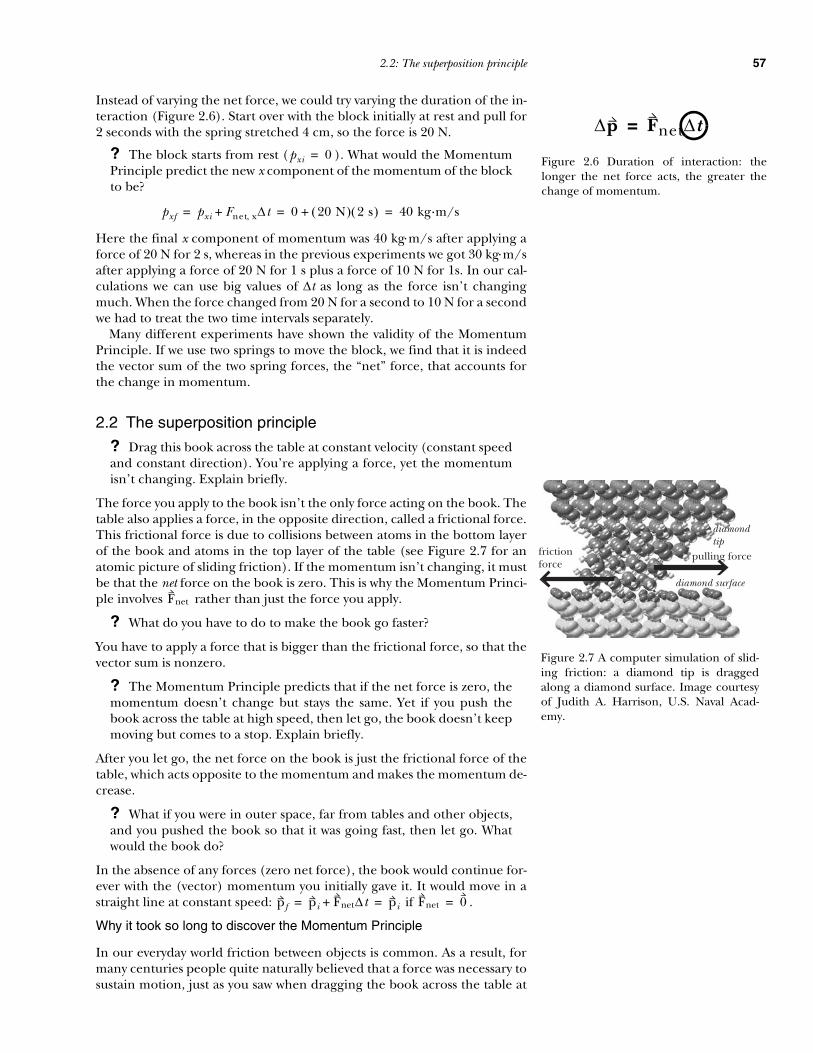
Instead of varying the net force, we could try varying the duration of the in-teraction (Figure 2.6). Start over with the block initially at rest and pull for2 seconds with the spring stretched 4 cm, so the force is 20 N.
? The block starts from rest ( ). What would the MomentumPrinciple predict the new x component of the momentum of the blockto be?
Here the final x component of momentum was 40 kg⋅m/s after applying aforce of 20 N for 2 s, whereas in the previous experiments we got 30 kg⋅m/safter applying a force of 20 N for 1 s plus a force of 10 N for 1s. In our cal-culations we can use big values of ∆t as long as the force isn’t changingmuch. When the force changed from 20 N for a second to 10 N for a secondwe had to treat the two time intervals separately.
Many different experiments have shown the validity of the MomentumPrinciple. If we use two springs to move the block, we find that it is indeedthe vector sum of the two spring forces, the “net” force, that accounts forthe change in momentum.
2.2 The superposition principle
? Drag this book across the table at constant velocity (constant speedand constant direction). You’re applying a force, yet the momentumisn’t changing. Explain briefly.
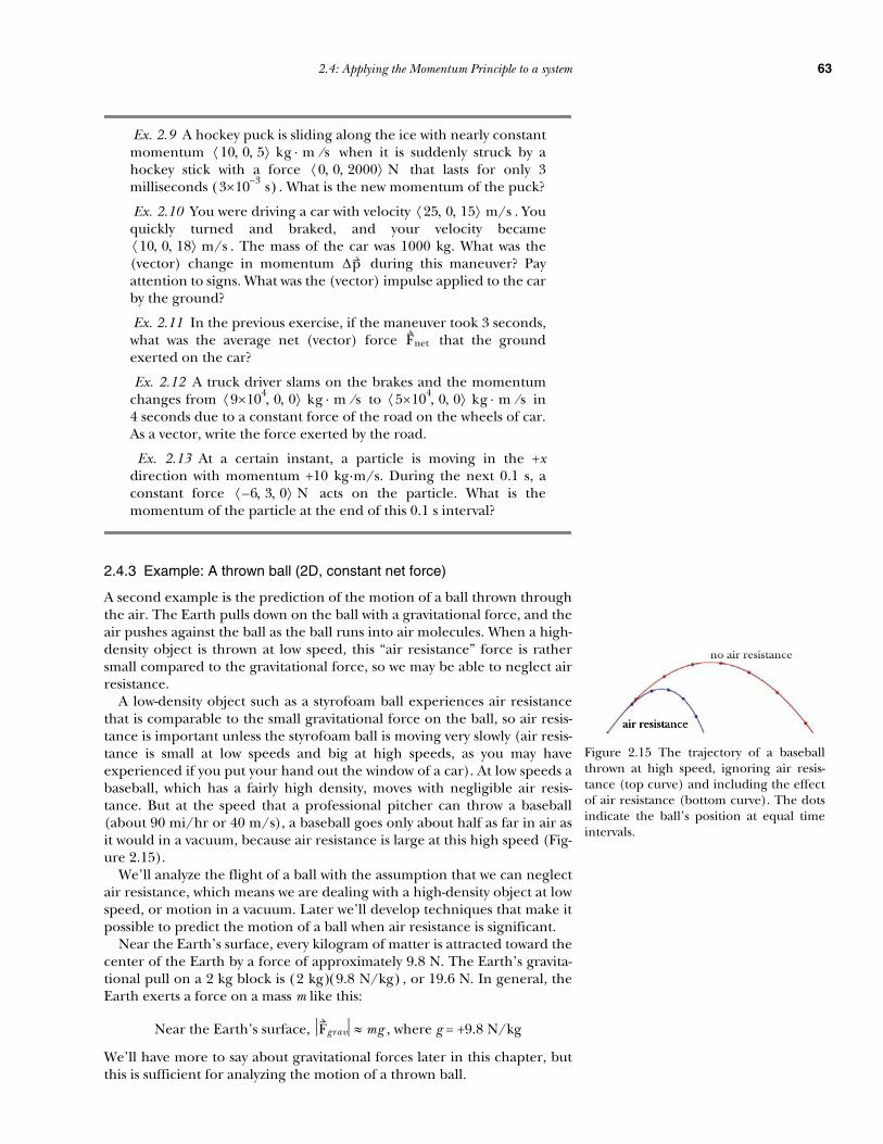
The force you apply to the book isn’t the only force acting on the book. Thetable also applies a force, in the opposite direction, called a frictional force.This frictional force is due to collisions between atoms in the bottom layerof the book and atoms in the top layer of the table (see Figure 2.7 for anatomic picture of sliding friction). If the momentum isn’t changing, it mustbe that the net force on the book is zero. This is why the Momentum Princi-ple involves rather than just the force you apply.
? What do you have to do to make the book go faster?
You have to apply a force that is bigger than the frictional force, so that thevector sum is nonzero.
? The Momentum Principle predicts that if the net force is zero, themomentum doesn’t change but stays the same. Yet if you push thebook across the table at high speed, then let go, the book doesn’t keepmoving but comes to a stop. Explain briefly.
After you let go, the net force on the book is just the frictional force of thetable, which acts opposite to the momentum and makes the momentum de-crease.
? What if you were in outer space, far from tables and other objects,and you pushed the book so that it was going fast, then let go. Whatwould the book do?
In the absence of any forces (zero net force), the book would continue for-ever with the (vector) momentum you initially gave it. It would move in astraight line at constant speed: if .
Why it took so long to discover the Momentum Principle
In our everyday world friction between objects is common. As a result, formany centuries people quite naturally believed that a force was necessary tosustain motion, just as you saw when dragging the book across the table at
Figure 2.6 Duration of interaction: thelonger the net force acts, the greater thechange of momentum.
∆p Fnet∆t=
pxi 0=
pxf pxi Fnet x, ∆t+ 0 20 N( ) 2 s( )+ 40 kg·m/s= = =
diamondtip
friction force
pulling force
diamond surface
Figure 2.7 A computer simulation of slid-ing friction: a diamond tip is draggedalong a diamond surface. Image courtesyof Judith A. Harrison, U.S. Naval Acad-emy.
Fnet
pf pi Fnet∆t+ pi= = Fnet 0=

58 Chapter 2: The Momentum Principle
constant speed. This made it hard to understand what made the planetskeep moving. Galileo and Newton finally realized that it is the net force thatmatters, and that objects free of interactions just naturally keep moving,with no forces needed to keep them moving (Newton’s first law of motion).This represented a major revolution in how humans viewed the world.
2.2.1 Net force
How do we calculate the net force acting on an object? It turns out to be sur-prisingly straightforward, as summarized by the superposition principle.
THE SUPERPOSITION PRINCIPLE
The net force on an object is the vector sum of theindividual forces exerted on it by all other objects.
Each individual interaction is unaffected bythe presence of other interacting objects.
The superposition principle is completely general. It has been found exper-imentally to apply to all kinds of interactions: gravitational, electromagnet-ic, and nuclear interactions. The implications of this principle are notalways intuitively obvious. For example, this principle implies that the forceexerted by the Sun on the Earth at a particular distance will always be thesame, regardless of how many other planets there are that also interact withthe Sun and the Earth. The presence of other objects and interactions doesnot block or change the interactions between each pair of objects. An inter-action doesn’t get “used up,” and the interaction between one object andanother is unaffected by the presence of a third object.
To take a silly example, hold a glass over a table and then let go (Figure2.8). The glass falls, so evidently the table doesn’t block the gravitational in-teraction with the Earth. In fact, the table adds a tiny additional gravitation-al force on the glass to that of the Earth, without changing the Earth’sattraction for the glass.
Ex. 2.5 A balloon experiences a gravitational force of and a force due to the wind of .
What is the net force acting on the balloon? Ex. 2.6 A sailboat sails straight toward an island at constant speed.What are all the forces acting on the boat? Is the net force zero ornonzero? Ex. 2.7 You watch someone carry a heavy block left-to-right acrossthe room, walking at constant speed. According to the MomentumPrinciple, should we conclude that the net force acting on the blockis upward, toward the right, or zero?
2.3 System and surroundings
In order to use the Momentum Principle to predict motion, we must choosea “system” whose momentum change we will calculate. By the word “system”we mean some pieces of the Universe of interest to us. The rest of the Uni-verse we call the “surroundings” (Figure 2.9).
To predict the motion of a baseball through the air, it makes sense tochoose the baseball as the system whose momentum changes. The sur-roundings include the Earth which exerts a gravitational force on our cho-sen system (the baseball), and the air, which exerts a force of air resistance
Figure 2.8 The presence of the table doesnot change the interaction of the glasswith the Earth.
0 0.05– 0, ,⟨ ⟩ N 0.03– 0 0.02, ,⟨ ⟩ N
SYSTEM
SURROUNDINGS
SURROUNDINGS SURROUNDINGS
SURROUNDINGS
Figure 2.9 System and surroundings. Inter-actions in the form of impulses flow acrossthe system boundary and change the sys-tem’s momentum.

2.3: System and surroundings 59
against the moving ball (Figure 2.10). It is true that there are changes in themomentum of the Earth and the momentum of the air molecules due to in-teractions with the baseball, but once we decide to choose the baseball asthe system of interest we don’t have to pay attention to what happens to themomentum of objects in the surroundings. The role of the surroundings isdescribed entirely by the forces they exert on our chosen system.
Only external forces matter
It is an important rule that we do not include in the net force acting on thebaseball any forces that the baseball exerts on itself. The atoms of the base-ball do exert forces on each other, but as we’ll discuss in more detail later,interatomic forces and gravitational force come in equal and opposite pairs(Figure 2.11). Therefore these “internal” force pairs, forces between pairsof atoms internal to our chosen system, add up to zero and can safely be ig-nored in calculating the net force that appears in the Momentum Principle,
. Only “external” forces matter, forces associated with inter-actions between our chosen system and objects in the surroundings.
Of course objects in the surroundings experience forces exerted by ob-jects inside the system, but when we apply the Momentum Principle just tothe system, we only care about the change of momentum of the system. Al-so, there are equal and opposite changes of momentum in the surround-ings, but they typically don’t interest us.
Neglecting small effects
The surroundings of the system of the baseball includes the Sun, the Moon,Mars, etc. Do we have to consider all of the forces these objects exert on thebaseball? In practice, no, because these forces are extremely small com-pared to the forces exerted on the system by the Earth and the air duringthe brief flight of the baseball. But if we were trying to plot an accuratecourse for a spacecraft going to Mars we would need to include even smallforces exerted by other planets, because impulse is forces times time dura-tion, , and in the long time required to go to Mars even small forces canproduce significant impulses, and significant changes in the momentum ofthe spacecraft.
Systems consisting of several objects
A system can consist of more than one object. For example, we mightchoose to consider a system consisting of the entire Solar System. The sur-roundings of this large system would include the rest of the Universe, in-cluding neighboring stars. The total momentum of the Solar System canchange due to the gravitational forces exerted by stars, especially nearbystars.
Ex. 2.8 In Section 2.1.3 we applied the Momentum Principle topredict the motion of a glider on an air track. What did we chooseas the system in this analysis? What objects were included in thesurroundings?
System is baseball
Earth is part of surroundings
Air is part of surroundings
Figure 2.10 Choose a baseball as the sys-tem. The surroundings are the Earth andthe air, which interact across the systemboundary to change the momentum of thesystem.
p
pf pi Fnet∆t+=
Internal forces cancel;no effect on system momentum
External forces changethe system momentum
System
Object insurroundings
Figure 2.11 Internal force pairs cancel, soonly external forces can change themomentum of a system.
Fon 2 by 1
Fon 1 by 2
F∆t

60 Chapter 2: The Momentum Principle
2.4 Applying the Momentum Principle to a system
To apply the Momentum Principle to analyze the motion of a real-world sys-tem, several steps are required:
1. Choose a system, consisting of a portion of the Universe.The rest of the Universe is called the surroundings.
2. List objects in the surroundings that exert significant forces on the chosen system, and make a labeled diagram showing the external forcesexerted by the objects in the surroundings.
3. Apply the Momentum Principle to the chosen system:
For each term in the Momentum Principle, substitute any values you know.
4. Apply the position update formula, if necessary:
5. Solve for any remaining unknown quantities of interest.
6. Check for reasonableness (units, etc.).
2.4.1 Example: Position and momentum of a ball
Inside a spaceship in outer space there is a small steel ball of mass 0.25 kg.At a particular instant, the ball is located at position and has mo-mentum . At this instant the ball is being pulled by astring, which exerts a net force on the ball. What is the ball’sapproximate momentum and position 3 milliseconds later ?What approximations or simplifying assumptions did you make in your anal-ysis?
A labeled diagram (step 3) gives a physicsview of the situation, and it defines sym-bols to use in writing an algebraic state-ment of the Momentum Principle.
pf pi Fnet∆t+=
rf ri varg∆t+=
9 5 0, ,⟨ ⟩ m8– 3 0, ,⟨ ⟩ kg·m/s
20 50 0, ,⟨ ⟩ N3 3–×10 s( )
ball
Fstring
1. Choose a system
System: the steel ball
2. List external objects that interact with the system, with diagram
the string(a circle represents the system)
3. Apply the Momentum Principle
pf pi Fnet∆t+=
pf 8– 3 0, ,⟨ ⟩ kg·m/s( ) 20 50 0, ,⟨ ⟩ N( ) 3 3–×10 s( )+=
pf 8– 3 0, ,⟨ ⟩ kg·m/s( ) 0.06 0.15 0, ,⟨ ⟩ N·s( )+=
pf 7.94– 3.15 0, ,⟨ ⟩ kg·m/s=
Assume that the force didn’t change muchduring 3 ms. Or to put it another way, weassumed that a time interval of 3 ms wassufficiently short that we could update themomentum fairly well assuming a constantforce during that short time interval.

2.4: Applying the Momentum Principle to a system 61
2.4.2 Example: A fan cart (1D, constant net force)
An easy way to arrange to apply a nearly constant force is to mount an elec-tric fan on a cart (Figure 2.12). If the fan blows backwards, the interactionwith the air pushes the cart forward with a nearly constant force, making thecart’s momentum continually increase. Swamp boats used in the very shal-low Florida Everglades are built in a similar way, with large fans on top ofthe boats propelling them through the swamp.
When a fan cart or boat gets going very fast, air resistance becomes im-portant and at high speeds is as big as the propelling force, so that the netforce becomes zero, at which point the momentum doesn’t increase anymore, and the cart or boat travels at constant speed. For simplicity we’ll con-sider the motion at low speed, with negligible air resistance, so we can makethe approximation that the net force is due solely to the fan and is nearlyconstant.
(Note that the y component of the net force is zero, because the down-ward gravitational force on the cart is exactly balanced by the upward forceexerted by the track on the cart. In a later chapter we will examine the in-teraction between solid objects like the cart and the track in more detail.)
Predict new position and new momentum
Suppose you have a fan cart whose mass is 400 grams (0.4 kg), and with thefan turned on, the net force acting on the cart, due to the air and frictionwith the track, is N and constant. You give the cart a shove, andyou release the cart at position m with initial velocity m/s. What is the position of the cart 3 seconds later, and what is its momen-tum at that time?
4. Apply the position update formula
, where since v << c
5. There are no remaining unknowns
6. Check
Units check (momentum: kg·m/s and position: m)
rf ri varg∆t+= v p m⁄≈
rf 9 5 0, ,⟨ ⟩ m( ) 7.94– 3.15 0, ,⟨ ⟩ kg·m/s( )0.25 kg( )
----------------------------------------------------------------- 3 3–×10 s( )+=
rf 9 5 0, ,⟨ ⟩ m( ) 0.0953– 0.0378 0, ,⟨ ⟩ m( )+=
rf 8.905 5.038 0, ,⟨ ⟩ m=
We used the momentum at the end of theinterval to update the position.
Note that at very high speeds, isn’tvalid for updating position. See page 98.
v p m⁄≈
Figure 2.12 A fan cart on a track.
0.2 0 0, ,⟨ ⟩0.5 0 0, ,⟨ ⟩ 1.2 0 0, ,⟨ ⟩
1. Choose a system
System: the cart (including the fan)
2. List external objects that interact with the system, with diagram
the Earth, the track, the air(represent the system by a circle)
Fair
Ftrack
FEarth
cart

62 Chapter 2: The Momentum Principle
Approximating the average velocityIn order to use the position update formula, we need the average velocity ofthe cart. How do we find ? We know initial and final values for :
Can we use these values to find ? You may have guessed that the averagevelocity is the “arithmetic” (pronounced “arithMETic”) average:
The arithmetic average.is often a good approximation, but it is not alwaysexactly equal to the average velocity . The arithmetic averagedoes lie between the two extremes. For example, the arithmetic average of6 and 8 is (6+8)/2 = 14/2 = 7, halfway between 6 and 8. See Figure 2.13.
The arithmetic average does not give the true average velocity unless thevelocity is changing at a constant rate, which is the case only if the net forceis constant, as it happens to be for a fan cart. For example, if you drive 50mi/hr for four hours, and then 20 mi/hr for an hour, you go 220 miles, andyour average speed is (220 mi)/(5 hr) = 44 mi/hr, whereas the arithmeticaverage is (50+20)/2 = 35 mi/hr. In situations where the force is not con-stant, we have to choose short enough time intervals that the velocity is near-ly constant during the brief (see Figure 2.14).
APPROXIMATE AVERAGE VELOCITY
(if v << c)
exactly true only if changes at a constant rate ( constant)
The proof (which is more complicated than one might expect) is given inoptional Section 2.11 at the end of this chapter.
3. Apply the Momentum Principle
pf pi Fnet∆t+ pi Ftrack FEarth Fair+ +( ) ∆t( )+= =
pf 0.4kg( ) 1.2m s⁄( ) 0 0, ,⟨ ⟩ 0.2 Ftrack FEarth–( ) 0, ,⟨ ⟩N 3 s( )+≈
pf 1.08 0 0, ,⟨ ⟩ kg m s⁄⋅≈
Since , we can use the approximationthat .
Since the y component of the cart’s mo-mentum does not change, we know thatthe y component of the net force must bezero, and .
We can use a large time interval ∆t be-cause the force isn’t changing very muchin either magnitude or direction.
v c«p mv≈
Ftrack FEarth=
vavg v
vi 1.2 0 0, ,⟨ ⟩m s⁄=
vfpf
m----≈ 1.08 0 0, ,⟨ ⟩ kg m s⁄⋅
0.4 kg----------------------------------------------------- 2.7 0 0, ,⟨ ⟩m s⁄= =
vavg
vavgvi vf+( )
2-------------------≈
ti tft
vfx
vix
vx
(vix + vfx)2
Figure 2.13 vx is changing linearly withtime, so the arithmetic average is equal to
vavg ∆r ∆t⁄=
ti tft
vfx
vix
(vix + vfx)2
Figure 2.14 vx is not changing linearly withtime. In this case the arithmetic average ismuch higher than the average value of vx.
∆t
vavgvi vf+( )
2-------------------≈
v Fnet
4. Apply the position update formula
5. There are no remaining unknowns
6. Check
Position: m (correct units); , as it should be.
vavgvi vf+( )
2-------------------
1.2 2.7+( )2
-------------------------- 0 0+( )2
----------------- 0 0+( )2
-----------------, ,⟨ ⟩ ms-----= =
vavg 1.95 0 0, ,⟨ ⟩m s⁄ =
rf ri varg∆t+ 0.5 0 0, ,⟨ ⟩m 1.95 0 0, ,⟨ ⟩ ms
----- 3s( )+= =
rf 6.35 0 0, ,⟨ ⟩m=
xf xi>
The net force on the cart is constant, sothis calculation of average velocity givesthe correct value.
2.4: Applying the Momentum Principle to a system 63
Ex. 2.9 A hockey puck is sliding along the ice with nearly constantmomentum when it is suddenly struck by ahockey stick with a force that lasts for only 3milliseconds . What is the new momentum of the puck?
Ex. 2.10 You were driving a car with velocity . Youquickly turned and braked, and your velocity became
. The mass of the car was 1000 kg. What was the(vector) change in momentum during this maneuver? Payattention to signs. What was the (vector) impulse applied to the carby the ground?
Ex. 2.11 In the previous exercise, if the maneuver took 3 seconds,what was the average net (vector) force that the groundexerted on the car?
Ex. 2.12 A truck driver slams on the brakes and the momentumchanges from to in4 seconds due to a constant force of the road on the wheels of car.As a vector, write the force exerted by the road.
Ex. 2.13 At a certain instant, a particle is moving in the +xdirection with momentum +10 kg·m/s. During the next 0.1 s, aconstant force acts on the particle. What is themomentum of the particle at the end of this 0.1 s interval?
2.4.3 Example: A thrown ball (2D, constant net force)
A second example is the prediction of the motion of a ball thrown throughthe air. The Earth pulls down on the ball with a gravitational force, and theair pushes against the ball as the ball runs into air molecules. When a high-density object is thrown at low speed, this “air resistance” force is rathersmall compared to the gravitational force, so we may be able to neglect airresistance.
A low-density object such as a styrofoam ball experiences air resistancethat is comparable to the small gravitational force on the ball, so air resis-tance is important unless the styrofoam ball is moving very slowly (air resis-tance is small at low speeds and big at high speeds, as you may haveexperienced if you put your hand out the window of a car). At low speeds abaseball, which has a fairly high density, moves with negligible air resis-tance. But at the speed that a professional pitcher can throw a baseball(about 90 mi/hr or 40 m/s), a baseball goes only about half as far in air asit would in a vacuum, because air resistance is large at this high speed (Fig-ure 2.15).
We’ll analyze the flight of a ball with the assumption that we can neglectair resistance, which means we are dealing with a high-density object at lowspeed, or motion in a vacuum. Later we’ll develop techniques that make itpossible to predict the motion of a ball when air resistance is significant.
Near the Earth’s surface, every kilogram of matter is attracted toward thecenter of the Earth by a force of approximately 9.8 N. The Earth’s gravita-tional pull on a 2 kg block is , or 19.6 N. In general, theEarth exerts a force on a mass m like this:
Near the Earth’s surface, , where g = +9.8 N/kg
We’ll have more to say about gravitational forces later in this chapter, butthis is sufficient for analyzing the motion of a thrown ball.
10 0 5, ,⟨ ⟩ kg m⋅ s⁄0 0 2000, ,⟨ ⟩ N
3 3–×10 s( )
25 0 15, ,⟨ ⟩ m/s
10 0 18, ,⟨ ⟩ m/s∆p
Fnet
9 4×10 0 0, ,⟨ ⟩ kg m⋅ s⁄ 5 4×10 0 0, ,⟨ ⟩ kg m⋅ s⁄
6 3 0, ,–⟨ ⟩ N
no air resistance
Figure 2.15 The trajectory of a baseballthrown at high speed, ignoring air resis-tance (top curve) and including the effectof air resistance (bottom curve). The dotsindicate the ball’s position at equal timeintervals.
2 kg( ) 9.8 N/kg( )
Fgrav mg≈

64 Chapter 2: The Momentum Principle
Predict new velocity and new position of a thrown ball
You throw the ball so that just after it leaves your hand at location it has velocity , with no component in the z direction. Now thatit has left your hand, and we’re neglecting air resistance, the net force at alltimes is , since the Earth’s gravitational force acts downward, to-ward the center of the Earth, and we normally choose our axes so y pointsup. Predict the velocity and position of the ball after a time . .
? Under what circumstances can we use this result to predict thetrajectory of an object?
We assumed that air resistance was negligible, that the object was travelingat a speed much less than the speed of light, and that the net force was con-stant. If any of these three conditions are not met, then these results do notapply, and using them will give a wrong answer.
xi yi 0, ,⟨ ⟩vxi vyi 0, ,⟨ ⟩
0 mg– 0, ,⟨ ⟩
∆t
ball
FEarth
Fair
1. Choose a system
System: the ball
2. List external objects that interact with the system, with diagram
the Earth, the air(represent the system by a circle)
3. Apply the Momentum Principle
4. Apply the position update formula
Alternatively:
5. There are no remaining unknowns
6. Check
The units check for the final position. Note that g is N/kg, so that is N·s/kg, units of impulse/kg, which is kg·m/s/kg, or m/s.
pf pi Fnet∆t+=
m vxf vyf 0, ,⟨ ⟩ m vxi vyi 0, ,⟨ ⟩ 0 mg– 0, ,⟨ ⟩∆t+=
vxf vyf 0, ,⟨ ⟩ vxi vyi 0, ,⟨ ⟩ 0 g– 0, ,⟨ ⟩∆t+=
vxi 0∆t+( ) vyi g– ∆t+( ) 0 0 ∆t( )+( ), ,⟨ ⟩=
vxi vyi g– ∆t+( ) 0, ,⟨ ⟩=
vargvxi vxi+
2-------------------⎝ ⎠
⎛ ⎞ vyi vyi g– ∆t+( )+( )2
---------------------------------------------- 0 0+( )2
-----------------, ,⟨ ⟩=
varg vxi vyi12---g∆t–( ) 0, ,⟨ ⟩=
rf ri varg∆t+=
xf yf 0, ,⟨ ⟩ xi yi 0, ,⟨ ⟩ vxi vyi12---g∆t–( ) 0, ,⟨ ⟩∆t+=
xf yf 0, ,⟨ ⟩ xi vxi∆t+( ) yi vyi∆t 12---g ∆t( )2–+( ) 0, ,⟨ ⟩=
xf xi vxi∆t+=
yf yi vyi∆t 12---g ∆t( )2–+=
zf 0=
g∆t
We make the approximation that air resis-tance is negligible compared to the gravita-tional force.
so v c« p mv≈
Divide both sides of the equation by m
The x and z components of velocity are notchanging; this makes sense because the netforce has only a y component. The y com-ponent of velocity is decreasing continu-ously; this makes sense because thegravitational force on the ball by the Earthaffects the y component of the ball’s veloc-ity.

2.4: Applying the Momentum Principle to a system 65
Using this result
If a ball of mass 90 g is initially on the ground, at location , andyou kick it with initial velocity , where will the ball be half a sec-ond later?
? Can we use these equations to find the location of the ball 10seconds after you kick it?
No. Our result would be that the ball was far underground:
which is not physically reasonable! (The ball would have hit the ground andstopped before 10 seconds had passed.)
? What should you remember from the preceding example?
If you understand the basic method, you can reproduce the specific resultsquickly and accurately. Just memorizing the results won’t help you much,because you won’t really understand what they mean or when they can beused.
For concreteness we analyzed the flight of a thrown ball, but this sameanalysis would work for any situation where an object moves in two dimen-sions under the influence of a constant net force. For example, just bychanging the constant y component of the net force to be something otherthan , we could analyze the two-dimensional motion of a swamp boat(if the direction of the thrust of the propeller doesn’t change, and we canneglect friction with the water), or to the two-dimensional motion of anelectron between two large charged plates. However, in these cases, the re-sulting equations would be slightly different, because the mass of the objectwould appear in the result (the m cancels only in the case of a force that isproportional to m, such as the gravitational force).
Graphs of the motion.
In Figure 2.16 we shows graphs of position and velocity components vs.time, and the actual path (y vs. x) of the ball. The first graph, vs. t, is sim-ply a horizontal line, because doesn’t change, since there is no x compo-nent of force. The graph of x is a straight line (second graph), rising if is positive. Note that the slope of the x vs. t graph is equal to .
The graph of is a falling straight line (third graph), because the y com-ponent of the force is , which constantly makes the y component of mo-mentum decrease. At some point the y component of momentum decreasesto zero, at the top of the motion, after which the ball heads downward, withnegative . The graph of y vs. time t is an inverted parabola (fourth graph),since the equation for y is a quadratic function in the time.
Note that the slope of the y vs. t graph (the fourth graph) at any time isequal to at that time. In particular, when the slope is zero (at the maxi-mum y), is momentarily equal to zero. Before that point the slope is pos-itive, corresponding to > 0, and after that point the slope is negative,corresponding to < 0.
The actual path of the ball, the graph of y vs. x, is also an inverted parab-ola (the bottom graph). Since x increases linearly with t, whether we plot yvs. t or y vs. x we’ll see a similar curve. The scale factor along the horizontalaxis is different, of course (meters instead of seconds).
0 0 0, ,⟨ ⟩ m3 7 0, ,⟨ ⟩ m/s
xf 0 3m s⁄( ) 0.5 s( )+ 1.5 m= =
yf 0 7m s⁄( ) 0.5 s( ) 9.8N kg⁄( ) 0.5 s( )2–+ 1.05 m= =
yf 7m s⁄( ) 10 s( ) 9.8N kg⁄( ) 10 s( )2– 910 m–= =
mg–
t
vx
vx does not change
∆t
vxi
ti tf
t
vy
vy continually decreases
Stops rising,heads downward
Rising, vy > 0
Falling, vy < 0
vyi
vyf
ti tf
t
x
x increases at constant ratexi
xf
ti tf
t
y
Rising
Stops rising,heads downward
Falling
This is y vs. time t. It is not the path.
yi
yf
ti tf
x
yActual path: y vs. x
yi
yf
xi xf
< xi, yi, 0 >
< xf, yf, 0 >
Figure 2.16 Graphs for the thrown ball.
vxvx
vxvx
vymg–
vy
vyvy
vyvy

66 Chapter 2: The Momentum Principle
Understanding the results
Let’s explore the results a bit to understand what they tell us about the mo-tion. The x component of the motion is very simple; it is completely unaf-fected by the downward-pointing gravitational force, so x simply increases ata constant rate ( constant). Of course, once the ball hits the ground, x nolonger increases.
The y component of the motion is more interesting. The equation
says that if you throw the ball so that is positive (heading up), at sometime will decrease to zero, and then become negative.
? At what time will the ball reach its highest point?
Our result for y as a function of time:
does not help us answer this question, because we don’t yet know how highthe ball will go (we don’t know what to use for ).
? Can we use the equation for as a function of time to find the timeat which the ball reaches its highest point? Do we know the value
of when the ball reaches its highest point?
Just before the ball reaches its maximum height, is positive. Just after itreaches its maximum height and begins to head downward, is negative.At the instant the ball reaches its maximum height, . Using this in-formation, we can solve for the elapsed time at that instant:
If then
? How high is the ball when it turns around and heads downward?
Now that we have a value for , we can use that in our general result forthe final position:
is the maximum height above your hand
Check the algebra yourself to verify this result. This result makes sense, inthat the bigger the initial y component of velocity, the higher the ball willgo. Notice that it doesn’t matter at all what x component of initial velocityyou give the ball; all that matters is . However, it takes more effort to givethe ball some in addition to giving it some , so for maximum heightyou want to throw the ball nearly straight up.
? Suppose you throw the ball so that it rises 2 m before falling backdown. If you double , how far will it rise above your hand?
Since , doubling will make the ball go up 4 times ashigh, to 8 m above your hand.
? Suppose you throw the ball so that it rises 2 m on Earth. If you givethe ball the same on the Moon, where g is about one-sixth that onEarth, how far will the ball rise above your hand?
vx
vyf vyi g∆t–=
vyivy
∆ttop
yf yi vyi∆t 12---g ∆t( )2–+=
yf
vy∆ttop
vy
vyvy
vy 0=
vyf vyi g∆ttop– 0= = ∆ttopvyi
g------=
∆ttop
yf yi vyi∆ttop12---g ∆ttop( )2–+ yi vyi
vyi
g------⎝ ⎠
⎛ ⎞ 12---g
vyi
g------⎝ ⎠
⎛ ⎞2
–+= =
yf yi–vyi
2
2g------=
vyivxi vyi
vyi
yf yi– vyi2 2g( )⁄= vyi
vyi

2.4: Applying the Momentum Principle to a system 67
Since , if g decreases by a factor of 6 but stays the same,the rise of the ball will increase by a factor of 6, so the ball will rise to 12 mabove your hand. Because there is no air on the Moon, our analysis workswell there.
? On Earth, what must you give the ball so that it rises 10 m aboveyour hand?
We have , and solving this we find. This is a high enough speed that air resistance might be sig-
nificant, and our result inaccurate.
? Suppose the ball is caught by a friend at the same height as youlaunched the ball. What is the formula for how long the ball was in theair?
In this case we have , so gives us
; compare with
The ball takes twice as long to go up and down as to go up, so we concludethat the time to come down is the same as the time to go up. (In the pres-ence of air resistance, the speed at every height is slower on the way down,so it takes longer to come down than to go up.) Again, notice that the timeto go up and down doesn’t depend at all on the x component of velocity.The x and y motions are independent of each other.
? How far from you is your friend when the ball is caught? Note thatyou know how long the ball was in the air, and you know the xcomponent of velocity.
, so the distance is
This distance is called the “range” of the ball. It is the distance the ball goesin the air if it returns to the same height. It depends on because that de-termines how much time it spends in the air. The result also depends on because that determines how far the ball will move in the x direction whilethe ball is in the air.
Initial speed and angle
Sometimes you know the initial speed and angle θ for the launch of aball. Figure 2.17 shows how to calculate the sine and cosine of the angle.Use these results to solve for the velocity components:
,
Ex. 2.14 A ball is kicked from a location (on theground) with initial velocity .
(a) What is the velocity of the ball 0.6 seconds after being thrown?(b) What is the location of the ball 0.6 seconds after being thrown?(c) What is the maximum height reached by the ball?(d) At what time does the ball reach its maximum height?(e) At what time does the ball hit the ground?(f) What is the location of the ball when it hits the ground?
Ex. 2.15 Apply the general results obtained in the full analysis onpage 64 to answer the following questions. You hold a small metalball of mass m a height h above the floor. You let go, and the ballfalls to the floor. Choose the origin of the coordinate system to beon the floor where the ball hits, with y up as usual. Just after release,
yf yi– vyi2 2g( )⁄= vyi
vyi
10 m vyi2 2 9.8 N/kg( )( )⁄=
vyi 14 m/s=
yf yi= yf yi vyi12---g∆t–( )∆t+=
∆tup and down 2vyi
g------= ∆ttop
vyi
g------=
xf xi vxi∆tup and down+= xf xi– vxi 2vyi
g------⎝ ⎠
⎛ ⎞=
vyvx
θ
vi
Figure 2.17 Converting speed and angleto velocity components.
θcos adjhyp---------
vxi
v------= =
θsin opphyp----------
vyi
v------= =
vxi vi θcos=
vyi vi θsin=
v
vxi v θcos= vyi v θsin=
9 0 5–, ,⟨ ⟩ m10– 13 5–, ,⟨ ⟩ m/s

68 Chapter 2: The Momentum Principle
what are and ? Just before hitting the floor, what is ? Howmuch time does it take for the ball to fall? What is just beforehitting the floor? Express all results in terms of m, g, and h. Howwould your results change if the ball had twice the mass?
Ex. 2.16 A soccer ball is kicked at an angle of 60° to the horizontalwith an initial speed of 10 m/s. Assume that we can neglect airresistance. For how much time is the ball in the air? How far does itgo (horizontal distance along the field)? How high does it go?
2.4.4 Graphical prediction of motion
It is instructive to apply the Momentum Principle qualitatively and graphi-cally to the thrown ball, to see visually how the Momentum Principle deter-mines the motion. The Momentum Principle predicts that in a short timeinterval ∆t, the momentum of the ball will change by an amount
which we can calculate, because we know the force acting onthe ball. In the following diagram we show the initial momentum , thechange in the momentum , and the new momentum
. Note that this vector addition corresponds to adding the ar-rows and tip to tail. We approximate the average momentum in thetime interval by the new momentum , and we advance the ball in thedirection of .
During the short time interval ∆t, the ball will move an amount , inthe direction of its new velocity (we assume that v << c). The ve-locity is changing during this time interval, but if ∆t is quite small (as it couldbe if we let a computer do the calculations), the change in the velocity isquite small, and it doesn’t matter very much whether we use the velocity atthe start or end of the time interval, or some kind of average. In this partic-ular case of constant net force the average velocity is the arithmetic average,but if we included air resistance the net force wouldn’t be constant in mag-nitude or direction, yet this method would still be accurate as long as we usesmall .
At the next position we repeat the procedure, graphically adding the vec-tors and to obtain the new momentum . We then ad-vance the ball in the direction of . As we do this repeatedly, we trace outgraphically the trajectory of the ball. You can see that the trajectory lookslike what is observed in the real world, and you can even see the increasingmagnitude of the ball as it falls, corresponding to increasing speed. The im-portant point to see in the diagram is that the net impulse changesthe momentum.
yi vyi yf∆t vyf
∆p Fnet∆t=p1
∆p Fnet∆t=p2 p1 ∆p+=
p1 ∆p∆t p2
Graphical prediction of the motion of aball, for three successive time steps.
p2
p1
∆p Fnet∆t=
p4
p3
p2
Fnet
p2
p3
p4
p5
Fnet
Fnet
Fnet
∆p Fnet∆t=
∆p Fnet∆t=
∆p Fnet∆t=
v∆tv2 p2 m⁄=
∆t
p2 ∆p Fnet∆t= p3p3
Fnet∆t
2.4: Applying the Momentum Principle to a system 69
2.4.5 Example: Block on spring (1D, nonconstant net force)
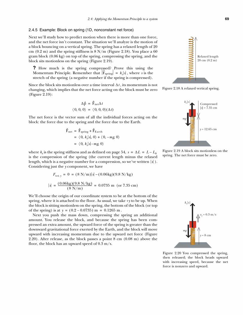
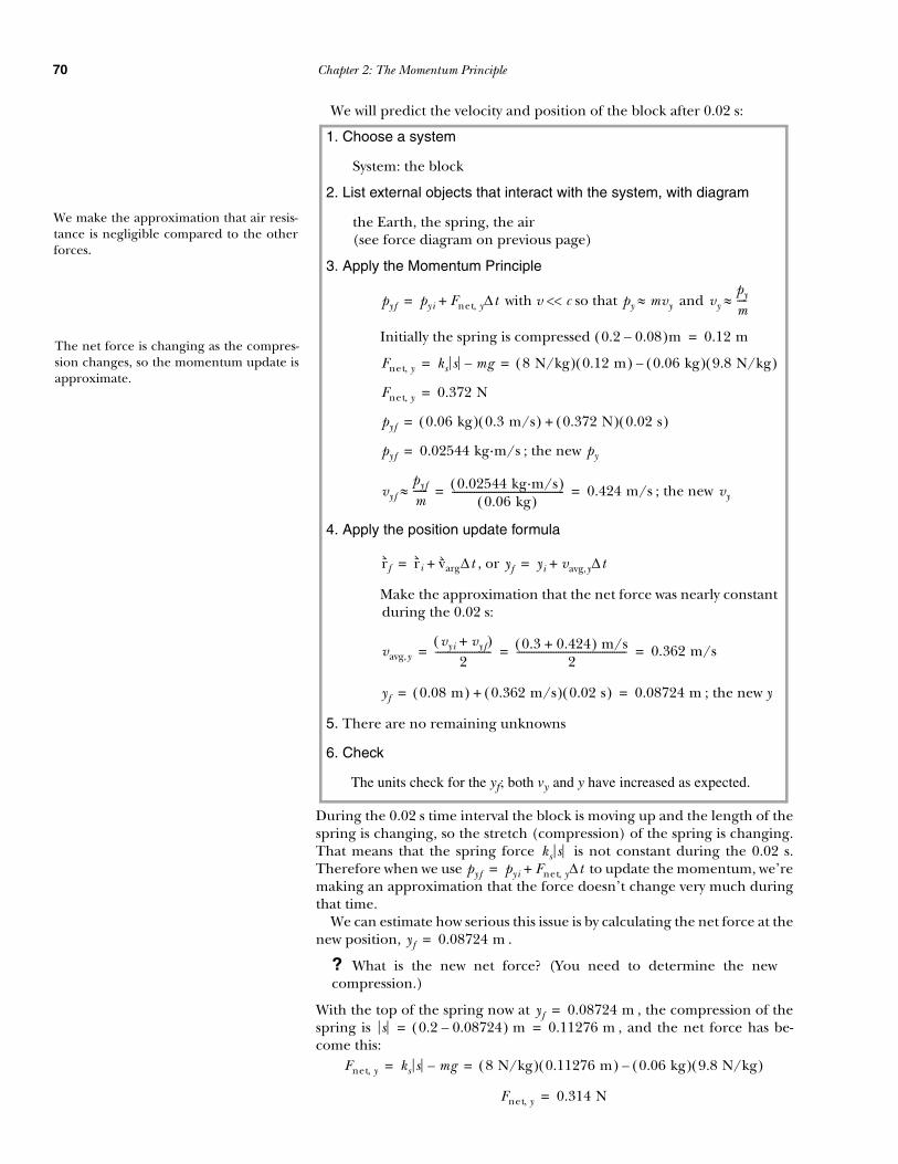
Next we’ll study how to predict motion when there is more than one force,and the net force isn’t constant. The situation we’ll analyze is the motion ofa block bouncing on a vertical spring. The spring has a relaxed length of 20cm (0.2 m) and the spring stiffness is 8 N/m (Figure 2.18). You place a 60gram block (0.06 kg) on top of the spring, compressing the spring, and theblock sits motionless on the spring (Figure 2.19).
? How much is the spring compressed? Prove this using theMomentum Principle. Remember that , where s is thestretch of the spring (a negative number if the spring is compressed).
Since the block sits motionless over a time interval , its momentum is notchanging, which implies that the net force acting on the block must be zero(Figure 2.19):
The net force is the vector sum of all the individual forces acting on theblock: the force due to the spring and the force due to the Earth.
where ks is the spring stiffness and as defined on page 54, is the compression of the spring (the current length minus the relaxedlength, which is a negative number for a compression, so we’ve written ).Considering just the y component, we have
(or 7.35 cm)
We’ll choose the origin of our coordinate system to be at the bottom of thespring, where it is attached to the floor. As usual, we take +y to be up. Whenthe block is sitting motionless on the spring, the bottom of the block (or topof the spring) is at .
Next you push the mass down, compressing the spring an additionalamount. You release the block, and because the spring has been com-pressed an extra amount, the upward force of the spring is greater than thedownward gravitational force exerted by the Earth, and the block will moveupward with increasing momentum due to the upward net force (Figure2.20). After release, as the block passes a point 8 cm (0.08 m) above thefloor, the block has an upward speed of 0.3 m/s.
Relaxed length20 cm (0.2 m)
Figure 2.18 A relaxed vertical spring.
Fspring ks s=
Compressed|s| = 7.35 cm
y = 12.65 cm
mg
ks|s|
Figure 2.19 A block sits motionless on thespring. The net force must be zero.
∆t
∆p Fnet∆t=
0 0 0, ,⟨ ⟩ 0 0 0, ,⟨ ⟩ ∆t( )=
Fnet Fspring FEarth+=
0 ks s 0, ,⟨ ⟩ 0 mg– 0, ,⟨ ⟩+=
0 ks s mg– 0, ,⟨ ⟩=
s ∆L L L0–= =
s
Fnet y, 0 8 N/m( ) s 0.06kg( ) 9.8 N/kg( )–= =
s 0.06kg( ) 9.8 N/kg( )8 N/m( )
--------------------------------------------------- 0.0735 m= =
y 0.2 0.0735–( ) m 0.1265 m= =
mg
ks|s|
y = 8 cm
vy = 0.3 m/s
Figure 2.20 You compressed the spring,then released; the block heads upwardwith increasing speed, because the netforce is nonzero and upward.
70 Chapter 2: The Momentum Principle
We will predict the velocity and position of the block after 0.02 s:
During the 0.02 s time interval the block is moving up and the length of thespring is changing, so the stretch (compression) of the spring is changing.That means that the spring force is not constant during the 0.02 s.Therefore when we use to update the momentum, we’remaking an approximation that the force doesn’t change very much duringthat time.
We can estimate how serious this issue is by calculating the net force at thenew position, .
? What is the new net force? (You need to determine the newcompression.)
With the top of the spring now at , the compression of thespring is , and the net force has be-come this:
1. Choose a system
System: the block
2. List external objects that interact with the system, with diagram
the Earth, the spring, the air(see force diagram on previous page)
3. Apply the Momentum Principle
with v << c so that and
Initially the spring is compressed
; the new
; the new
4. Apply the position update formula
, or
Make the approximation that the net force was nearly constant during the 0.02 s:
; the new y
5. There are no remaining unknowns
6. Check
The units check for the yf; both vy and y have increased as expected.
pyf pyi Fnet y, ∆t+= py mvy≈ vypy
m----≈
0.2 0.08–( )m 0.12 m=
Fnet y, ks s mg– 8 N/kg( ) 0.12 m( ) 0.06 kg( ) 9.8 N/kg( )–= =
Fnet y, 0.372 N=
pyf 0.06 kg( ) 0.3 m/s( ) 0.372 N( ) 0.02 s( )+=
pyf 0.02544 kg·m/s= py
vyfpyf
m------≈ 0.02544 kg·m/s( )
0.06 kg( )---------------------------------------------- 0.424 m/s= = vy
rf ri varg∆t+= yf yi vavg,y∆t+=
vavg,yvyi vyf+( )
2----------------------- 0.3 0.424+( ) m/s
2--------------------------------------------- 0.362 m/s= = =
yf 0.08 m( ) 0.362 m/s( ) 0.02 s( )+ 0.08724 m= =
We make the approximation that air resis-tance is negligible compared to the otherforces.
The net force is changing as the compres-sion changes, so the momentum update isapproximate.
ks spyf pyi Fnet y, ∆t+=
yf 0.08724 m=
yf 0.08724 m=s 0.2 0.08724–( ) m 0.11276 m= =
Fnet y, ks s mg– 8 N/kg( ) 0.11276 m( ) 0.06 kg( ) 9.8 N/kg( )–= =
Fnet y, 0.314 N=

2.4: Applying the Momentum Principle to a system 71
The net force at the start of the time interval was . So al-though the net force did change during the 0.02 s, it didn’t change verymuch, and our approximate analysis is therefore pretty good.
? How could our predictions be improved?
By taking shorter time steps. Instead of taking one step of 0.02 s, we couldtake two steps of 0.01 s, or ten steps of 0.002 s. During each of these shortertime intervals the compression would change less, so the force would bemore nearly constant. Unfortunately, to achieve increased accuracy we haveto do a lot more calculations.
Taking another step
To continue predicting the motion of the block into the future, we can takeanother step. The final values of momentum and position after the original0.02 s step become the initial values for the next 0.02 s step:
Look through this calculation and make sure you understand how the fi-nal results for position and momentum from the first 0.02 s time step havebeen used as the initial values for the second 0.02 s time step.
In principle we could continue, taking more and more steps to predictfarther and farther into the future. Here is a summary of this iterativescheme:
Fnet y, 0.372 N=
3. Apply the Momentum Principle
with v << c so that and
Spring is compressed
; the new
; the new
4. Apply the position update formula
, or
Make the approximation that the net force was nearly constant during the 0.02 s:
pyf pyi Fnet y, ∆t+= py mvy≈ vypy
m----≈
0.2 0.08724–( )m 0.11276 m=
Fnet y, ks s mg–8 N/kg( ) 0.11276 m( ) 0.06 kg( ) 9.8 N/kg( )–
==
Fnet y, 0.314 N=
pyf 0.02544 kg·m/s( ) 0.314 N( ) 0.02 s( )+=
pyf 0.03172 kg·m/s= py
vyfpyf
m------≈ 0.03172 kg·m/s( )
0.06 kg( )---------------------------------------------- 0.5287 m/s= = vy
rf ri varg∆t+= yf yi vavg,y∆t+=
vavg,yvyi vyf+( )
2----------------------- 0.424 0.5287+( ) m/s
2------------------------------------------------------- 0.4764 m/s= = =
yf 0.08724 m( ) 0.4764 m/s( ) 0.02 s( )+ 0.09677 m= =
The initial momentum and position aretaken from the final momentum and posi-tion in the previous step.
• Start with initial positions and momenta of the interacting objects.• Calculate the (vector) forces acting on each object.• Update the momentum of each object: .• Update the positions: .• Repeat.
pf pi Fnet∆t+=rf ri varg∆t+=

72 Chapter 2: The Momentum Principle
Every time you repeat, the “final” momentum and position become the “ini-tial” momentum and position for the next step. You have to use an approx-imate value for , either by using the velocity at the start or end of thetime interval, or by taking the arithmetic average of these two velocities aswe did above.
While this scheme is very general, doing it by hand is incredibly tedious.It is possible to program a computer to do these calculations repetitively.Computers are now fast enough that it is possible to get high accuracy sim-ply by taking very short time steps, so that during each step the net force andvelocity aren’t changing much. We’ll talk more about computer predictionof motion later in this chapter.
Ex. 2.17 After a third time step of 0.02 seconds, what will be theposition and momentum of the block?
2.4.6 Example: Fast proton (1D, constant net force, relativistic)
A proton in a particle accelerator is moving with velocity , sothe speed is . A constant electric force isapplied to the proton to speed it up, . What is theproton’s speed as a fraction of the speed of light after 20 nanoseconds( )?
The speed didn’t increase very much, because the proton’s initial speed,0.96c, was already close to the cosmic speed limit, c. Because the speed hard-ly changed, the distance the proton moved during the 20 ns was approxi-mately equal to .
varg
0.96c 0 0, ,⟨ ⟩0.96 3 8×10× m/s 2.88 8×10 m/s=
Fnet 5 12–×10 0 0, ,⟨ ⟩ N=
1 ns 1 9–×10 s=
proton
1. Choose a system
System: the proton
2. List external objects that interact with the system, with diagram
electric charges in the accelerator(a circle represents the system)
3. Apply the Momentum Principle
Evaluate (no units)
pf pi Fnet∆t+=
pxf 0 0, ,⟨ ⟩ γimvxi 0 0, ,⟨ ⟩ 5 12–×10 0 0, ,⟨ ⟩ N( ) 20 9–×10 s( )+=
pxf1
1 0.96cc
-------------⎝ ⎠⎛ ⎞
2–
---------------------------------- 1.7 27–×10 kg( ) 0.96 3 8×10× m/s( ) 1 19–×10 N·s( )+=
pxf 1.75 18–×10 kg·m/s( ) 1 19–×10 N·s( )+ 1.85 18–×10 kg·m/s= =
vxf
c------
pxf
mc------
1pxf
mc------⎝ ⎠
⎛ ⎞2
+
----------------------------=
pxf
mc------ 1.85 18–×10 kg·m/s
1.7 27–×10 kg( ) 3 8×10 m/s( )---------------------------------------------------------------------- 3.62= =
vxf
c------ 3.62
1 3.622+--------------------------- 0.964= =
5 12–×10 0 0, ,⟨ ⟩ N
(See Section 2.15, page 98; obtaining v from pwhen the speed is near the speed of light.)
0.96 3 8×10 m/s×( ) 20 9–×10 s( ) 5.8 m=
2.5: Problems of greater complexity 73
2.5 Problems of greater complexity
So far all of the examples we have considered have involved finding achange in momentum (and position), given a known force acting over aknown time interval. The following problems require you to find either theduration of an interaction (time interval), or the force exerted during aninteraction. These large problems involve several steps in reasoning.
2.5.1 Example: Strike a hockey puck
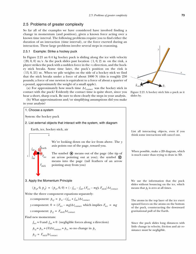
In Figure 2.21 an 0.4 kg hockey puck is sliding along the ice with velocity As the puck slides past location on the rink, a
player strikes the puck with a sudden force in the +z direction, and the hock-ey stick breaks. Some time later, the puck’s position on the rink is
. When we pile weights on the side of a hockey stick we findthat the stick breaks under a force of about 1000 N (this is roughly 250pounds; a force of one newton is equivalent to a force of about a quarter ofa pound, approximately the weight of a small apple).
(a) For approximately how much time was the hockey stick incontact with the puck? Evidently the contact time is quite short, since youhear a short, sharp crack. Be sure to show clearly the steps in your analysis.
(b) What approximations and/or simplifying assumptions did you makein your analysis?
xz
y
Figure 2.21 A hockey stick hits a puck as itslides by.
piFstick
20 0 0, ,⟨ ⟩ m/s 1 0 2, ,⟨ ⟩ m
13 0 21, ,⟨ ⟩ m
∆tcontact
1. Choose a system
System: the hockey puck
2. List external objects that interact with the system, with diagram
Earth, ice, hockey stick, air
3. Apply the Momentum Principle
Write the three component equations separately:
x component:
y component: which implies
z component:
Find new momentum:
and (negligible forces along x direction)
so no change in
We’re looking down on the ice from above. The yaxis points out of the page, toward you.
The symbol means out of the page (the tip ofan arrow pointing out at you); the symbol means into the page (tail feathers of an arrowpointing away from you)
z
x
Fice
fair
Fstick
FEarth
fair
pxf 0 pzf, ,⟨ ⟩ pxi 0 0, ,⟨ ⟩ fice– fair– Fice mg–( ) Fstick, ,⟨ ⟩∆tcontact+=
pxf pxi fice fair+( )∆tcontact–=
0 Fice mg–( )∆tcontact= Fice mg=
pzf Fstick∆tcontact=
fice 0≈ fair 0≈
pxf pxi 0( )∆tcontact pxi≈+≈ px
pzf Fstick∆tcontact=
List all interacting objects, even if youthink some interactions will cancel out.
We use the information that the puckslides without bouncing on the ice, whichmeans that py is zero at all times.
The atoms in the top layer of the ice exertupward forces on the atoms on the bottomof the puck, counteracting the downwardgravitational pull of the Earth.
Since the puck slides long distances withlittle change in velocity, friction and air re-sistance must be negligible.
When possible, make a 2D diagram, whichis much easier than trying to draw in 3D.

74 Chapter 2: The Momentum Principle
? Given these results from the Momentum Principle for and ,make a sketch of the path of the puck before and after it is hit.
The path of the puck must look something like that shown in Figure 2.22.In the result there are two unknowns, and .
We need another equation in order to be able to solve for the unknown con-tact time . We can get additional information from the position up-date formula .
How good were our approximations?
We made the following approximations and simplifying assumptions:• Ice exerts little force in the x or z directions; low sliding friction.• Negligible air resistance.• Force of stick is roughly constant during and equal to 1000 N.• The puck doesn’t move very far during the contact time.
The neglect of sliding friction and air resistance is probably pretty good,since a hockey puck slides for long distances on ice.
We know the hockey stick exerts a maximum force of Fstick = 1000 N, be-cause we observe that the stick breaks. We approximate the force as nearlyconstant during contact. Actually, this force grows quickly from zero at firstcontact to 1000 N, then abruptly drops to zero when the stick breaks.
The final approximation is somewhat questionable. Although 0.013 s is ashort time, the puck moves (20 m/s)(0.013 s) = 0.26 m (a bit less than onefoot) in the x direction during this time. Also during this time increasesfrom 0 to 31.7 m/s, with an average value of about 15.8 m/s, so the z dis-placement is about (15.8 m/s)(0.013 s) = 0.2 m during contact. On the oth-er hand, these displacements aren’t very large compared to thedisplacement from to , so our result isn’t terribly
px pz
z
xinitial < 1, 0, 2 > m
final < 13, 0, 21 > m
Figure 2.22 The x component of themomentum (and velocity) hardly changes,but the z component of momentum (andvelocity) changes quickly from zero tosome final value when the puck is hit.
pzf Fstick∆tcontact= pzf Fstick
∆tcontactrf ri vavg∆t+=
4. Apply the position update formula
In , let be the amount of time it takes the puck toslide from where it was struck to the known final position:
x component: , so
y component: so (not a surprise)
z component: since , so
5. Solve for the unknowns
where (since v << c)
6. Check
• Units check (contact time is in seconds)• Is the result reasonable? The contact time is very short, as expected.
If for example it had come out to be 300 s (5 minutes!) we shouldcheck our calculations.
rf ri varg∆t+= ∆tslide
13 0 21, ,⟨ ⟩ m 1 0 2, ,⟨ ⟩ m( ) 20 m/s 0 vz, ,⟨ ⟩∆tslide+=
13 m( ) 1 m( ) 20 m/s( )∆tslide+=
∆tslide 12 m( ) 20 m/s( )⁄ 0.6 s= =
0 0 0∆tslide+= 0 0=
21 m( ) 2 m( ) vz 0.6 s( )+= ∆tslide 0.6 s=
vz 19 m( ) 0.6 s( )⁄ 31.7 m/s= =
pzf Fstick∆tcontact= pzf mvzf≈
0.4 kg( ) 31.7 m/s( ) 1000 N( )∆tcontact=
∆tcontact 0.4 kg( ) 31.7 m/s( ) 1000 N( )⁄ 0.013 s= =
Since the puck slides long distances withlittle change in velocity, friction and airresistance must be negligible. We assumethat after the puck is struck, the velocityis nearly constant (with a new magnitudeand direction). Therefore the average ve-locity is the same as the velocity just afterimpact.
The contact time is very short, a smallfraction of a second. As a result, you heara short sharp crack when the stick hits thepuck.
∆tcontact
vz
1 0 2, ,⟨ ⟩ m 13 0 21, ,⟨ ⟩ m

2.5: Problems of greater complexity 75
inaccurate due to this approximation. Nevertheless, a more accurate sketchof the path of the puck should show a bend as in Figure 2.23.
We can even calculate the radius of curvature of this bend, the radius ofthe “kissing circle” discussed in the previous chapter. We know that
On the left, since
At first contact the velocity is in the x direction and has magnitude of 20m/s. The kissing circle is tangent to the incoming velocity.
On the right,
Equate the left and right quantities:
Solve:
This is a plausible result for the radius of the bend, since we saw that xchanges by about 0.26 m and z changes by about 0.2 m during contact.
It is important to see that even though our analysis of the stick contacttime (0.013 s) isn’t exact, it is adequate to get a reasonably good determina-tion of this short time, something that we wouldn’t know without using theMomentum Principle and the position update formula. The short durationof the impact explains why we hear a sharp, short crack.
Choice of system
? We chose the hockey puck as the system to analyze. Why not choosethe system consisting of both the hockey puck and the hockey stick?
The problem with choosing both objects as the system is that the 1000 Nforce is now an internal force and doesn’t show up in the Momentum Prin-ciple, so we aren’t able to use this information. By the reciprocity of electricforces, including the interatomic forces between stick and puck, the puckexerts a 1000 N force on the stick. In the combined system the puck gainsmomentum from the stick, and the stick loses momentum to the puck. Thetotal momentum of the system doesn’t change: .
Review
Let’s review what we did to analyze this situation, in the form of a generalscheme for attacking problems. We can summarize our work with a diagramin the shape of a diamond, which emphasizes
• starting from the Momentum Principle applied to a system, • then expanding for the particular situation, • then contracting down to solving for the quantity of interest, • followed by checking for reasonableness.
z
x
Figure 2.23 A more accurate overhead viewof the path of the hockey puck, showingthe bend during impact.
dpdt------ Fnet=
dpdt------
vR----- p m v 2
R------------≈ 0.4 kg( ) 20 m/s( )2
R-----------------------------------------------= = p mv≈
Fnet 1000 N=
0.4 kg( ) 20 m/s( )2
R----------------------------------------------- 1000 N=
R 0.4 kg( ) 20 m/s( )2
1000 N( )----------------------------------------------- 0.16 m= =
psystem 0=

76 Chapter 2: The Momentum Principle
Link the lines in this diamond to the hockey stick analysis:
An important point implied by this diamond is that it is usually not useful totry to jump immediately to the step “Solve for the unknowns,” by huntingfor some formula that gives the unknown quantity directly. Very often sucha special-case formula may not exist. For example, in the hockey puck prob-lem the contact time emerged from applying the Momentum Principle andthe position update formula. There wasn’t some ready-made “formula forthe contact time for hockey sticks and pucks” that you could use.
If you start by applying the Momentum Principle to a chosen system youcan attack novel problems that you’ve never before encountered. The Mo-mentum Principle is always valid, whereas special-case formulas aren’t.
In previous studies you may have been taught a useful but restricted ap-proach to solving problems, which is to start with a formula for the unknownquantity. That is, if you’ve trying to find v, start with a formula for v. We willhelp you learn a more powerful technique for solving problems, which is tostart from a fundamental physics principle (in this case the MomentumPrinciple), expand it by substituting known values, then contract to solve forthe unknown quantities. In other words, you derive the formula you needrather than hunt for it. This is the only technique that can give you the pow-er to solve novel problems, ones that no one has previously encountered.
In an increasingly complex world, engineers and scientists are continuallybeing asked to meet new challenges. A major goal of this course is to pre-pare you to meet the novel challenges of the 21st century.
2.5.2 Example: Colliding students
Next we’ll work through in detail a messy real-world situation: Two studentswho are late for tests are running to classes in opposite directions as fast asthey can (Figure 2.24). They turn a corner, run into each other head-on,and crumple into a heap on the ground. Using physics principles, estimatethe force that one student exerts on the other during the collision. You willneed to estimate some quantities; give reasons for your choices and providechecks showing that your estimates are physically reasonable.
This problem is rather ill-defined and doesn’t seem much like a “text-book” problem. No numbers have been given, yet you’re asked to estimatethe force of the collision. This kind of problem is typical of the kinds ofproblems engineers and scientists encounter in their professional work. Forexample, suppose you are trying to design a crash helmet and you need toestimate the force it must withstand without breaking. You don’t know ex-actly what the ultimate wearer will be doing at the time of a crash, so youhave to make some reasonable estimates of typical human activities onwhich to base your analysis. We’ll make the simplifying assumption that thestudents have similar masses and similar speeds (Figure 2.24).
1. Choose a system.
2. List interacting objects, with diagram.
3. Apply the Momentum Principle:
Expand the Momentum Principle by substituting any values you know.
4. You may also need to expand .
5. Solve for the unknowns.
6. Check.
pf pi Fnet∆t+=
rf ri varg∆t+=
v v
m m
Figure 2.24 Colliding students. The speed(magnitude of velocity) of each student isassumed to be the same and is representedby v. We also make the simplifying assump-tion that the students have about the samemass m.

2.5: Problems of greater complexity 77
Remember the diamond scheme as a guide to how to proceed. We’ll car-ry out the analysis symbolically and plug in estimated values of student massand speed at the end. That way we get a general solution that can be evalu-ated for different values of these quantities.
We could estimate the typical mass of a student, and the likely speed of astudent running at full speed, but is one equation in two un-knowns, the unknown force F of the other student and the time duration
of the impact.
? Before trying to apply the position update formula ,try to estimate of the impact simply by making a guess.
It is common to guess what seems a rather short time, such as a second, orhalf a second. However, it is easy to show that such estimates are way off. Therecord for the 100 m dash is about 10 seconds. If we assume that these stu-dents are very fast runners, they each could be running 10 m/s. An alterna-tive way of making the estimate is to note that you can easily walk about 4miles in an hour, which gives
This moderate walking speed suggests that the students should be able torun between 5 m/s and 10 m/s. Let’s estimate that they each have a speed
. During the collision the speed drops quickly from v to 0, so theaverage speed during the collision is approximately , or 2.5 m/s.
? If we guess that is about half a second, during that half second,how far does the student move?
1. Choose a system
System: the student on the left
2. List external objects that interact with the system, with diagram
Earth, ground, other student, air
(more complex diagram shows pointof application of each force)
3. Apply the Momentum Principle
Write the three component equations separately:
x component:
y component: , so
z component: which is true but uninformative
Find new momentum:
Assume and are negligible compared to F
, so since v << c
0 0 0, ,⟨ ⟩ pxi 0 0, ,⟨ ⟩ F– fground fair–– Fground mg–( ) 0, ,⟨ ⟩∆t+=
0 pxi F fground fair+ +( )∆t–=
0 Fground mg–( )∆t= Fground mg=
0 0=
fground fair
0 pxi F∆t–= mv F∆t=
mg
F
fground
Fground
fair
List all interacting objects, even if youthink some interactions will cancel out.
Many of the momentum components arezero. Do you see why pxf = 0?
In a vector equation, the x component onthe left must equal the x component on theright; similarly for y and z.
The student’s heels are pushed to the leftalong the ground due to the collision, andthe resisting ground pushes to the right.We’ll assume that this force is much small-er than the force exerted by the other stu-dent, because the student’s shoes can slip.
mv F∆t=
∆t
rf ri varg∆t+=∆t
v 4 mihr--------⎝ ⎠
⎛ ⎞ 1.6 kmmi
---------⎝ ⎠⎛ ⎞ 1000 m
km--------⎝ ⎠
⎛ ⎞ 1 hr3600 s----------------⎝ ⎠
⎛ ⎞ 1.8 m/s≈≈
v 5 m/s≈v 0+( ) 2⁄
∆t

78 Chapter 2: The Momentum Principle
At an average speed of 2.5 m/s, in a half second the student would go 1.25meters, well over a yard. This would imply that the two students pass rightthrough each other, coming out the other side! Evidently an estimate of ahalf second is wildly too big and is inconsistent with the real world.
The problem is that it is very difficult to guess short time intervals accu-rately. On the other hand, we can estimate short distances rather well, andthis gives us an indirect way to estimate short time intervals. Each studentgets squeezed during the collision. Suppose each student’s body getspushed in a distance of about (try pushing on yourstomach and see how much deflection you can make).
15000 N is a very large force. For example, the gravitational force on a 60kg student (the “weight”) is only about . Theforce of the impact is more than 25 times the weight of the student! It’s likehaving a stack of 25 students sitting on you. If the students hit heads insteadof stomachs, the squeeze might be less than 1 cm, and the force would beover 5 times as large! This is why heads can break in such a collision.
So yes, our result of 15000 N is plausible: collisions involve very large forc-es acting for very short times, giving impulses of ordinary magnitude.
How good were our approximations?
We made the following approximations and simplifying assumptions:• We estimated the running speed from known 100 m dash records.• We estimated the masses of the students; we could plug in other masses
now that we have derived general results in terms of m and v.• We assumed that the horizontal component of the force of the ground
on the bottom of the student’s shoe was small compared to the forceexerted by the other student. Now that we find that the impact forceis huge, this assumption seems quite good.
• We made the approximation that the impact force was nearly constantduring the impact, so what we’ve really determined is an average force.
• We assumed that the students had similar masses and similar runningspeeds, to simplify the analysis. If this is not the case, the analysis is sig-nificantly more complicated, but we would still find that the impactforce is huge.
∆x 5 cm≈ 0.05 m=
4. Apply the position update formula
Apply or equivalently :
x component: , so
5. Solve for the unknowns
6. Check
• Units check (force is in newtons, collision time is in seconds)• Is the result reasonable? The contact time is very short, as expected.
Is the force reasonable or not? See discussion below.
rf ri vavg∆t+= vavg ∆r ∆t⁄=
v 2⁄ 0 0, ,⟨ ⟩ ∆x 0 0, ,⟨ ⟩ ∆t⁄=
v 2⁄ ∆x ∆t⁄= ∆t 2∆x v⁄=
mv F∆t F 2∆x v⁄( )= =
F mv2
2∆x---------- 60 kg( ) 5 m/s( )2
2 0.05 m( )------------------------------------------ 15000 N= = =
∆t 2∆xv
---------- 2 0.05 m( )5 m/s
-------------------------- 0.02 s= = =
Estimate that the student is brought to anabrupt stop in just 5 cm (about 2 inches).
The collision time is 25 times smallerthan our original guess of 0.5 s. So thekey to making a realistic estimate of atime interval is to estimate average speedand distance, and then derive a time esti-mate from that.
Force has units (kg)(m/s)/s, which hasthe units of momentum (kg·m/s) divid-ed by s, which is correct for a force(change of momentum divided by time).
60 kg( ) 9.8 N/kg( ) 600 N≈

2.5: Problems of greater complexity 79
You might object that with all these estimates and simplifying assumptionsthe final result of 15000 N for the impact force is fatally flawed. It is certainlythe case that we don’t have a very accurate result. But nevertheless wegained valuable information, that the impact force is very large. Before do-ing this analysis based on the Momentum Principle, we had no idea ofwhether the force was small compared to the student’s weight, comparable,or much bigger. Now we have a quantitative result that the force is on theorder of 25 times the weight of a student, and we can appreciate why colli-sions are so dangerous.
? What if we choose the system to include both students?
In this case there is almost no external impulse during the brief time of con-tact. The big internal forces the students exert on each other are equal inmagnitude but opposite in direction (due to the reciprocity of interatomicforces that come into play when the students make contact). Thereforethese forces don’t change the momentum of the combined system. Beforethe collision the total momentum of the combined system is zero( ), and after the collision the total momentum is also zero(they’re not moving). So there’s no change in momentum, which is consis-tent with there being negligible external forces. Simple analysis, but withthis choice of system we learn nothing about the force that one student ex-erts on the other. That’s why we choose just one student as the system.
2.5.3 Physical models
Our model of the colliding student situation is good enough for many pur-poses. However, we left out some aspects of the actual motion. For example,we mostly ignored the flexible structure of the students, how much theirshoes slip on the ground during the collision, etc. We have also quite sensi-bly neglected the gravitational force of Mars on the students, because it isso tiny compared to the force of one student on the other.
Making and using models is an activity central to physics, and the criteriafor a “good” physical model will depend on how we intend to use the model.In fact, one of the most important problems a scientist or engineer faces isdeciding what interactions must be included in a model of a real physical,chemical, or biological system, and what interactions can reasonably be ig-nored.
Simplified (or “idealized”) models
If we neglect some (hopefully small) effects, we say that we are constructinga simplified model of the situation. A useful model should omit extraneousdetail but retain the main features of the real-world situation. We hope thatthe main results of our analysis of the simplified model will apply adequatelyto the complex real-world situation.
Of course if we do a poor job of modeling and make inappropriate ap-proximations or neglect effects that are actually sizable, we may get a ratherinaccurate result (though perhaps adequate for some purposes). There istherefore a certain art to making a good model. One goal of this course isto help you develop skill in formulating simplified but meaningful physicalmodels of complex situations.
Another common way of describing a model is to say that it is an “ideali-zation,” by which we mean a simple, clean, stripped-down representation,free of messy complexities. “Ideally,” a ball will roll forever on a level floor,but a real ball rolling on a real floor eventually comes to a stop. An “ideal”gas is a fictitious gas in which the molecules don’t interact with each other,as opposed to a real gas whose molecules do interact, but only when theycome close to each other.
mv mv– 0=

80 Chapter 2: The Momentum Principle
The analysis of a simplified model gives an approximate result that differssomewhat from what actually happens in the real world. Alternatively, youcan consider your result to be exact for a different real-world situation, onewhere the neglected influences are not actually present. For example, thecalculations we made concerning the colliding students could apply almostexactly to two rubber balls moving in outer space that compress by theamount we estimated.
An important aspect of physical modeling that will engage us throughoutthis course is making appropriate approximations to simplify the messy,real-world situation enough to permit (approximate) analysis using New-ton’s laws. Actually, using Newton’s laws is itself an example of modelingand making approximations, because we are neglecting the effects of quan-tum mechanics and of general relativity (Einstein’s treatment of gravita-tion). Newton’s laws are only an approximation to the way the world works,though frequently an extremely good one.
2.6 Fundamental forces
There are four different kinds of fundamental forces currently known to sci-ence, associated with four different kinds of interactions: gravitational, elec-tromagnetic, nuclear (also referred to as the “strong” interaction), and the“weak” interaction.
• The gravitational interaction is responsible for an attraction every ob-ject exerts on every other object. For example, the Earth exerts a grav-itational force on the Moon, and the Moon exerts a gravitational forceon the Earth.
• The electromagnetic interaction includes electric forces responsible forsparks, static cling, and the behavior of electronic circuits, and mag-netic forces responsible for the operation of motors driven by electriccurrent. Protons repel each other electrically, as do electrons, whereasprotons and electrons attract each other (Figure 2.25). Electric forcesbind protons and electrons to each other in atoms, and are responsi-ble for the chemical bonds between atoms in molecules. The force ofa stretched or compressed spring is due to electric forces between theatoms that make up the spring.
• The nuclear or strong interaction holds protons and neutrons togetherin the nucleus of an atom despite the large mutual electric repulsionof the protons (Figure 2.26). (The neutrons are not electricallycharged and interact only through the strong force.)
• An example of the weak interaction is seen in the instability of a neu-tron. If a neutron is removed from a nucleus, with an average lifetimeof about 15 minutes the neutron decays into a proton, an electron,and a ghostly particle called the antineutrino. This change is broughtabout by the weak interaction.
We will be mainly concerned with gravitational and electric interactions, butwe will occasionally encounter situations where the nuclear or strong inter-action plays an important role. We will have little to say about the weak in-teraction. Nor will we deal with magnetism, the other part of theelectromagnetic interaction. The second volume of this textbook deals ex-tensively with both electric and magnetic interactions.
2.7 The gravitational force law
To predict the motion of stars, planets, spacecraft, comets, satellites, andother massive objects traveling through space, we need to use a gravitationalforce law together with the Momentum Principle. As a matter of general cul-
Figure 2.25 The electric force: protonsrepel each other; electrons repel eachother; protons and electrons attract eachother.
Figure 2.26 The strong force: the protonsin the nucleus of an atom exert repulsiveelectric forces on each other, but hestrong interaction holds the nucleustogether despite this electric repulsion.

2.7: The gravitational force law 81
ture, it can be interesting to understand how the motion of objects in spacecan be predicted by physics principles. If you are studying aerospace engi-neering or astrophysics this may also be a professional interest.
What if your interests are in nanotechnology or chemistry or civil engi-neering? Studying how to predict the motion of stars and planets is one ofthe most direct ways to understand in general how the Momentum Princi-ple determines the behavior of objects in the real world. The motion of starsand planets is in important ways simpler than other mechanical phenome-na, because there is no friction to worry about, so this is a good place to startyour study. The basic ideas used to predict the motion of stars and planetscan be applied later to a wide range of everyday and atomic phenomena.
In the 1600’s Isaac Newton deduced that there must be an attractive forceassociated with a gravitational interaction between any pair of objects. Thegravitational force acts along a line connecting the two objects (Figure2.27), is proportional to the mass of one object and to the mass of the otherobject, and is inversely proportional to the square of the distance betweenthe centers of the two objects (not the gap between their surfaces). Here isthe formula for the gravitational force exerted on object 2 by object 1:
THE GRAVITATIONAL FORCE LAW
points from the center of object 1 to the center of object 2
G is a universal constant:
This force law looks pretty complicated, but it could have been a lot morecomplicated than it is. For example, the gravitational force law does not de-pend on the momentum or velocity of the objects. It depends only on themasses, and on the position of one object relative to the other object.
Large spheres
An optional section at the end of this chapter (page 96) shows that uniform-density spheres interact gravitationally as though all of their mass were con-centrated at the center of the sphere, so the gravitational force law appliesto large uniform-density spheres as long as you use the center-to-center dis-tance. For example, the force that the Earth exerts on you can be calculatedas though all the mass of the Earth were at its center, away fromwhere you are sitting.
Measurement of G
Another optional section at the end of this chapter (page 97) tells how Cav-endish in the late 1700’s measured G by observing the tiny gravitationalforces two lead balls exerted on each other.
2.7.1 Understanding the gravitational force law
We will spend some time understanding how to calculate forces between ob-jects using Newton’s gravitational force law. Then we will use this force inthe Momentum Principle to predict the future motion of objects.
The gravitational force law involves a lot of different symbols and maylook pretty intimidating at first. Let’s take the law apart and look at the in-dividual pieces to try to make sense of the formula.
The relative position vector in the gravitational force law points fromthe center of object 1 to the center of object 2, and so does the unit vector
(“r-hat”) in Figure 2.28. Recall that in words is the location of ob-
m1
m2
Fgrav on 1 by 2
Figure 2.27 The gravitational force exertedon object 2 by object 1. (The force exertedon object 1 by object 2 has the same magni-tude but opposite direction.)
r2-1
Fgrav on 2 by 1 G–m2m1
r2-12
-------------- r̂2-1=
r̂2-1Fgrav on 2 by 1 G–m2m1
r2-12
------------- r̂2-1=
r2-1
G 6.7 11–×10 N m2⋅kg2
----------------=
6.4 6×10 m
m1
m2
Figure 2.28 The location of object 2 rela-tive to object 1: “final minus initial.”
r2-1 r2 r1–=
r1
r2
r̂2-1
r2-1
r̂2-1 r2-1

82 Chapter 2: The Momentum Principle
ject 2 relative to object 1, “final minus initial.” The magnitude of is thedistance between the centers of the two objects.
We say that the gravitational constant G is “universal” because it is thesame for any pair of interacting masses, no matter how big or small they are,or where they are located. Because G is universal, it can be measured for anypair of objects and then used with other pairs of objects. As we describe onpage 97, Cavendish was the first person to make such a measurement.
As highlighted in Figure 2.29, the gravitational force is proportional tothe product of the two masses, m2m1. If you double either of these masses,keeping the other one the same, the force will be twice as big. If you doubleboth of the masses, the force will be four times as big. Since m2m1 = m1m2,the magnitude of the force exerted on object 1 by object 2 is exactly thesame as the magnitude of the force exerted on object 2 by object 1 (but thedirection is opposite).
The gravitational force is an “inverse square” law. As highlighted in Figure2.30, the square of the center-to-center distance appears in the denomina-tor. This means that the gravitational force depends very strongly on the dis-tance between the objects. For example, if you double the distance betweenthem, the only thing that changes is the denominator, which gets four timesbigger (2 squared is 4), so the force is only 1/4 as big as before.
? If you move the masses 10 times farther apart than they wereoriginally, how does the gravitational force change?
The force goes down by a factor of 100. Evidently when two objects are veryfar apart, the gravitational forces they exert on each other will be vanishing-ly small: big denominator, small force.The minus sign with the unit vector highlighted in Figure 2.31 gives the di-rection of the force exerted on object 2 by object 1. The vector pointstoward object 2, as does the unit vector , and the force acting on object2 points in the opposite direction.
A useful way to think about the gravitational force law is to factor it intomagnitude and direction, like this:
• A vector is a magnitude times a direction:
• Magnitude:
• Direction (unit vector):
It is usually simplest to calculate the magnitude and direction separately,then combine them to get the vector force. That way you can focus on onething at a time rather than getting confused (or intimidated!) by the fullcomplexity of the vector force law.
Ex. 2.18 Masses M and m attract each other with a gravitationalforce of magnitude F. Mass m is replaced with a mass 3m, and it ismoved four times farther away. Now what is the magnitude of theforce?
Ex. 2.19 A 3 kg ball and a 5 kg ball are 2 m apart, center to center.What is the magnitude of the gravitational force that the 3 kg ballexerts on the 5 kg ball? What is the magnitude of the gravitationalforce that the 5 kg ball exerts on the 3 kg ball?
Ex. 2.20 Measurements show that the Earth’s gravitational forceon a mass of 1 kg near the Earth’s surface is 9.8 N. The radius of theEarth is 6400 km (6.4×10⁶ m). From these data determine the massof the Earth.
r2-1
Figure 2.29 The gravitational forcedepends on the product of the two masses.
G–m2m1
r2-12
-------------- r̂2-1
Figure 2.30 The gravitational force is an“inverse square” law.
G–m2m1
r2-12
-------------- r̂2-1
Figure 2.31 The direction of the gravita-tional force on object 2 is in the oppositedirection to the unit vector pointing towardobject 2.
G–m2m1
r2-12
-------------- r̂2-1 r2-1r̂2-1
Fgrav Fgrav F̂grav=
Fgrav Gm2m1
r2-12
-------------=
F̂grav r̂2-1–=
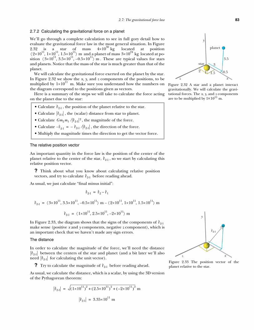
2.7: The gravitational force law 83
2.7.2 Calculating the gravitational force on a planet
We’ll go through a complete calculation to see in full gory detail how toevaluate the gravitational force law in the most general situation. In Figure2.32 is a star of mass located at position
and a planet of mass located at po-sition . These are typical values for starsand planets. Notice that the mass of the star is much greater than that of theplanet.
We will calculate the gravitational force exerted on the planet by the star.In Figure 2.32 we show the x, y, and z components of the positions, to bemultiplied by m. Make sure you understand how the numbers onthe diagram correspond to the positions given as vectors.
Here is a summary of the steps we will take to calculate the force actingon the planet due to the star:
The relative position vector
An important quantity in the force law is the position of the center of theplanet relative to the center of the star, , so we start by calculating thisrelative position vector.
? Think about what you know about calculating relative positionvectors, and try to calculate before reading ahead.
As usual, we just calculate “final minus initial”:
In Figure 2.33, the diagram shows that the signs of the components of make sense (positive x and y components, negative z component), which isan important check that we haven’t made any sign errors.
The distance
In order to calculate the magnitude of the force, we’ll need the distance between the centers of the star and planet (and a bit later we’ll also
need for calculating the unit vector).
? Try to calculate the magnitude of before reading ahead.
As usual, we calculate the distance, which is a scalar, by using the 3D versionof the Pythagorean theorem:
star
planet
2 1.5
3.5
1
3
-0.5
xz
y
Figure 2.32 A star and a planet interactgravitationally. We will calculate the gravi-tational forces. The x, y, and z componentsare to be multiplied by 1×10¹¹ m.
4 30×10 kg2 11×10 1 11×10 1.5 11×10, ,⟨ ⟩ m 3 24×10 kg
3 11×10 3.5 11×10 0.5 11×10–, ,⟨ ⟩ m
1 11×10
• Calculate , the position of the planet relative to the star.
• Calculate , the (scalar) distance from star to planet.
• Calculate , the magnitude of the force.
• Calculate , the direction of the force.
• Multiply the magnitude times the direction to get the vector force.
r2-1
r2-1
Gm2m1 r2-12⁄
r̂2-1– r2-1 r2-1⁄–=
r2-1
r2-1
r2-1 r2 r1–=
r2-1 3 11×10 3.5 11×10 0.5 11×10–, ,⟨ ⟩ m 2 11×10 1 11×10 1.5 11×10, ,⟨ ⟩ m–=
r2-1 1 11×10 2.5 11×10 2 11×10–, ,⟨ ⟩ m=
r2-1
r2-1r2-1
xz
y
Figure 2.33 The position vector of theplanet relative to the star.
r2-1
r2-1
r2-1 1 11×10( )2 2.5 11×10( )2 2 11×10–( )2+ + m=
r2-1 3.35 11×10 m=

84 Chapter 2: The Momentum Principle
The magnitude of the force
? Before reading ahead, try to calculate the magnitude of the force,.
The magnitude of the force on the planet by the star is this:
This looks like a big force, but it’s acting on a very big mass, so it isn’t obvi-ous whether this is really a “big” force in terms of what it will do.
The direction of the force
? Can you think how to calculate the vector direction of thegravitational force, the unit vector ? Try it.
We’ve got the magnitude of the force. We also need to calculate the direc-tion of the force, which involves the unit vector:
Direction of force:
Notice that the unit vector giving the direction has no units, because themeters in the numerator and the denominator cancel. Figure 2.34 showsthe unit vectors pointing from star toward planet, and from planet towardstar.
The vector gravitational force
? Try to construct the vector force. You know the magnitude, and youknow the direction.
Finally we can multiply the magnitude of the force times the unit vector di-rection of the force to get the full vector force:
Checking our result
It is important to check long calculations such as this, because there aremany opportunities to make a mistake along the way. There are severalchecks we can make.
• Diagram: An important check is to make a diagram like Figure 2.35 andsee whether the direction of the calculated force makes sense. Pay par-ticular attention to signs. The diagram shows that the force acting on
Fgrav on planet by star
Fgrav on planet by star Gm2m1
r2-12
-------------=
Fgrav on planet by star 6.7 11–×10 N m2⋅kg2
----------------⎝ ⎠⎛ ⎞ 3 24×10 kg( ) 4 30×10 kg( )
3.35 11×10 m( )2------------------------------------------------------------=
Fgrav on planet by star 7.16 21×10 N=
F̂grav on planet by star
F̂grav on planet by star r̂2-1– r2-1
r2-1----------–= =
F̂grav on planet by star 1 11×10 2.5 11×10 2 11×10–, ,⟨ ⟩ m
3.35 11×10 m------------------------------------------------------------------------------–=
F̂grav on planet by star 0.299– 0.746– 0.597, ,⟨ ⟩=
xz
y
Figure 2.34 Unit vectors.
r̂2-1
r̂2-1–
Fgrav on planet by star Fgrav on planet by star F̂grav on planet by star=
Fgrav on planet by star 7.16 21×10 N( ) 0.299– 0.746– 0.597, ,⟨ ⟩=
Fgrav on planet by star 2.14 21×10– 5.34 21×10– 4.27 21×10, ,⟨ ⟩ N=
xz
y
Figure 2.35 The gravitational force exertedon the planet by the star.
Fgrav on planet by star

2.7: The gravitational force law 85
the planet points in the , , direction, and this agrees with ourcalculation, which has the same component signs.
• Order of magnitude: Make a rough “order of magnitude” check, drop-ping all the detailed numbers. In terms of “order of magnitude” thedistance between star and planet is very roughly , the mass ofthe star is very roughly , the mass of the planet is very roughly
, and the gravitational constant is very roughly. Therefore we expect the magnitude of the force
to be very roughly this:
In this very rough order of magnitude calculation, ignoring numericaldetails, we just need to add and subtract exponents, and one hardlyeven needs a calculator. The fact that we get within an order of magni-tude of the result is evidence that we haven’t made anyhuge mistakes.
• Units: An important check is that the units came out correctly, in new-tons.
• Unit vector: Check to see whether the calculated unit vector does in-deed have magnitude 1:
The magnitude isn’t exactly 1 because we rounded off the intermediatecalculations to three significant figures.
Our result passes all these checks. This doesn’t prove we haven’t made amistake somewhere, but at least we’ve ruled out many possible errors.
The force on the star exerted by the planet
We’ve just calculated the force exerted on the planet by the star. To calcu-late the force exerted on the star by the planet, we could redo all theselengthy calculations in the same way, but that would be a lot of work.
? Look at the form of the gravitational force law and think carefully.Do you see a way to write down immediately the gravitational force onthe star by the planet, without doing any additional calculations?
Note that the magnitude is exactly the same, because it involves exactly thesame quantities. The only change is the direction of the force, which is inthe opposite direction. Therefore we can immediately write the new result,just by flipping the signs:
Note that the signs of the force components are consistent with Figure 2.36.You might be puzzled that the planet pulls just as hard on the star as the starpulls on the planet. We’ll discuss this in more detail later in this chapter.
How can you remember all these steps?
Calculating the vector gravitational force requires many steps, but each stepis pretty straight-forward. How can one remember what steps to take? Thinkof the equation for the gravitational force as a guide and outline for what todo.
x– y– +z
1 11×10 m1 30×10 kg
1 24×10 kg1 11–×10 N m2⋅ kg2⁄
1 11–×10 N m2⋅kg2
----------------⎝ ⎠⎛ ⎞ 1 24×10 kg( ) 1 30×10 kg( )
1 11×10 m( )2------------------------------------------------------------ 1 21×10 N=
7.16 21×10 N
F̂grav on planet by star 0.299–( )2 0.746–( )2 0.597( )2+ + 1.001= =
Fgrav on star by planet 2.14 21×10 5.34 21×10 4.27– 21×10, ,⟨ ⟩ N=
xz
y
Figure 2.36 The gravitational force exertedon the star by the planet.
Fgrav on star by planet
Fgrav on 2 by 1 G–m2m1
r2-12
------------- r̂2-1=
86 Chapter 2: The Momentum Principle
• When you look at the formula you see that you need , so you calcu-late it (“final minus initial”).
• You also see that you need , so you calculate that. • Now you see that you now have enough information to calculate the
magnitude of the force. • The formula tells you to calculate the negative of the unit vector, to get
the direction.• The formula says to multiply magnitude times direction. That’s it!
With this scheme in mind, look over the previous few pages to review howwe carried out the evaluation of the gravitational force law.
Ex. 2.21 The mass of the Earth is , and the mass of theMoon is . At a particular instant the Moon is at location
, in a coordinate system whose origin is atthe center of the Earth. (a) What is the relative position vector from the Earth to theMoon?(b) What is ?(c) What is the unit vector ?(d) What is the gravitational force exerted by the Earth on the Moon?Your answer should be a vector.
2.7.3 Using the gravitational force to predict motion
You now know that this star exerts this force on this planet at this instant,but what’s the point in knowing this? By itself, this isn’t particularly interest-ing. But if we use this calculated force in the Momentum Principle, we canpredict the future motion of the planet.
• We know the force at this instant, and if we know the initial momen-tum of the planet we can use the update form of the MomentumPrinciple, , to predict the momentum of the planet ashort time later. We need to choose short enough that the forcedoesn’t change much during this brief time interval, due to changesin the positions of the interacting objects.
• We can also use the velocity to update the position of the planet, usingthe position update formula . Again, we need tochoose short enough that the velocity doesn’t change much duringthat brief time interval, so that we can use the initial or final velocity asa good approximation to the average velocity.
After doing these momentum and position updates, we have successfullypredicted the new momentum and position a short time into the future.Now we can repeat this process, calculating a new gravitational force basedon the new position, updating the momentum, and updating the position.Step by step we can predict the motion of the planet into the future.
Although the massive star won’t move very much, we could also update itsmomentum and position repetitively. As we’ve seen, it’s easy to get the forceon the star just by flipping signs.
Here is a summary of this iterative scheme:
r2-1
r2-1
6 24×10 kg7 22×10 kg
2.8 8×10 0 2.8– 8×10, ,⟨ ⟩ m
rM-E
rM-Er̂M-E
pipf pi Fnet∆t+=∆t ∆t
rf ri varg∆t+=∆t
• Start with initial positions and momenta of the interacting objects.• Calculate the (vector) gravitational forces acting on each object.• Update the momentum of each object: .• Update the positions: , where .• Repeat.
pf pi Fnet∆t+=rf ri varg∆t+= varg pf m⁄≈

2.7: The gravitational force law 87
In order to plan the trajectory for a spacecraft from Earth to a particularlanding site on Mars, NASA has to carry out a very large number of such up-date calculations, taking small steps (small ) to achieve high accuracy.This includes calculating the net force as the vector sum of all the gravita-tional forces exerted on the spacecraft along the way by the Sun, Earth,Moon, Mars, and other objects in the Solar System. Doing all these forceand update calculations by hand would be impossibly difficult, so people atNASA write computer programs to do these repetitive calculations. Later wewill show you how to write such programs.
Updating the momentum and position of the planet
To see in detail how this iterative scheme works, we’ll carry out one com-plete step—one update of the momentum and position. In order to startthe iteration we have to know the initial positions and momenta of the starand planet. We already know their initial positions. Let’s suppose we alsoknow their initial velocities:
The star is initially at rest and, because it has a huge mass compared to theplanet, it won’t move very much. For simplicity we’ll make the approxima-tion that the star is fixed in position and never moves.
Choosing a sufficiently small time interval
We need to decide how big a value of we can get away with and yet pre-serve adequate accuracy. The smaller the time step , the more accuratethe calculation, because the force and velocity won’t change much duringthe brief time interval. However, taking smaller steps means doing more cal-culations to predict some time into the future.
Here is a way to choose a time interval. The initial speed is about. Choose a so that the distance the planet goes in this time
interval, , is small compared to the distance d between star and planet,which is about . As the planet changes position the gravitationalforce will change in magnitude and direction, as you can see in Figure 2.37.In the Momentum Principle we need for to be smallenough that is nearly constant during this time interval.
Let’s choose as a tentative criterion that the distance the planet movesought to be about 0.001 times the distance from the star to the planet:
This is about 3 hours. If instead we choose a large time interval of ,say, in the first update the planet would move a long distance, about
, which is about as large as the distanceto the star, and during that step the actual gravitational force would changea great deal in magnitude and direction. This would make our predictionsvery inaccurate.
Whenever you choose a time interval to use for updating momentum,make sure it is sufficiently small that the net force doesn’t change very muchin magnitude or direction during your chosen time interval.
∆t
vi ,star 0 0 0, ,⟨ ⟩ m/s=
vi,planet 1 4×10 2 4×10 1.5 4×10, ,⟨ ⟩ m/s=
∆t∆t
v 3 4×10 m/s≈ ∆tv∆t
3 11×10 m
pf pi Fnet∆t+= ∆tFnet
d
v∆t
Figure 2.37 If ∆t is too big, the gravitationalforce will change a lot in magnitude anddirection during the time interval.
v
Fat time t1
Fat time t2
v∆t 0.001d≈
∆t 0.001dv
-----------------≈ 0.001( ) 3 11×10 m( )
3 4×10 m/s( )------------------------------------------------ 1 4×10 s= =
1 7×10 s
3 4×10 m/s( ) 1 7×10 s( ) 3 11×10 m=
88 Chapter 2: The Momentum Principle
On the other hand, if the force happens to be constant in magnitude anddirection, you can use as large a as you like without making an error inthe momentum update.
Update the momentum of the planet
? We know the force acting on the planet, and we’ve chosen a timeinterval to make one step in predicting the future of the planet. Try topredict the momentum the planet will have after .
The planet is moving at a high speed, about , but this is smallcompared to the speed of light, which is , so the initial momen-tum is .
Use the Momentum Principle in its update form:
Notice that the momentum didn’t change very much, because we deliber-ately chose a small time interval to ensure accuracy in the momentum up-date, by making sure that the force remained nearly constant during thebrief time interval.
Update the position of the planet
? Think about how you would update the position of the planet.
We must use the position update formula, , but what is theaverage velocity ? The velocity (and momentum) changed during the
time step. Should we use the initial velocity? The final velocity? Thearithmetic average of these two velocities?
A key point is that the momentum changed very little, so the velocitychanged very little. Therefore it hardly matters which velocity we use. To beconcrete about this, and for simplicity in computer calculations, we’ll nor-mally use the final velocity (obtained from the just-calculated final momen-tum) to represent the average velocity. This works well as long as the timestep is small. Since , , and the position update is this:
∆t
1 4×10 s
3 4×10 m/s3 8×10 m/s
pi mvi≈
pi mvi≈ 3 24×10 kg( ) 1 4×10 2 4×10 1.5 4×10, ,⟨ ⟩ m/s( )=
pi 3 28×10 6 28×10 4.5 28×10, ,⟨ ⟩ kg·m/s=
pf pi Fnet∆t+=
pf 3 28×10 6 28×10 4.5 28×10, ,⟨ ⟩ kg·m/s
2.14 21×10– 5.34 21×10– 4.27 21×10, ,⟨ ⟩ N( ) 1 4×10 s( )+=
pf 2.9979 28×10 5.9947 28×10 4.5043 28×10, ,⟨ ⟩ kg·m/s=
rf ri varg∆t+=varg
1 4×10 s
pf mvf≈ vf pf m⁄≈
rf ripf
m----∆t+≈
rf 3 11×10 3.5 11×10 0.5 11×10–, ,⟨ ⟩ m( )
2.9979 28×10 5.9947 28×10 4.5043 28×10, ,⟨ ⟩ kg·m/s( )
3 24×10 kg( )---------------------------------------------------------------------------------------------------------------------------------- 1 4×10 s( )
+⎝
⎠
⎜
⎟
⎛
⎞
=
rf 3.001 11×10 3.502 11×10 0.4985 11×10–, ,⟨ ⟩ m=

2.7: The gravitational force law 89
What have we done?
Whew! After all that computational drudgery, what have we accomplished?We’ve predicted the future of the planet!
Knowing the planet’s initial position and momentum, we predict that af-ter the planet will be in a new position that we’ve calculated, with anew momentum that we’ve calculated. So what? Well, we could do thisagain. The second time step would involve exactly the same calculations wejust did, but the “initial” position and momentum would be the “final” oneswe just calculated. We could keep going, doing this over and over and over,and predict as far ahead into the future as we are willing to do the tediouscalculations.
You say you’d rather not do all those calculations? Right! The thing to dois to instruct a computer to do this for you. What you need to do is learn howto write out one set of instructions for the computer to do repetitively, overand over. Next we will show you how to do this, but it was important to guideyou once through the gory details of the calculation, so that you could un-derstand exactly what it is you have to tell the computer to do.
2.7.4 Telling a computer what to do
Here we summarize how to organize a computer program in order to tell acomputer how to apply the Momentum Principle repetitively to predict thefuture.
The details of the actual program statements depend on what program-ming language or system you use, and your instructor will provide you withthe details of the particular tool you will use.
A computer calculation
In the preceding sections you took one step in such a calculation, by hand.Figure 2.38 shows the orbit of the planet as predicted by a computer pro-gram written using VPython (http://vpython.org) that continually updatedthe momentum and position of the planet, repeatedly using the gravitation-al force law, the Momentum Principle, and the position update formula.The star and planet are shown much larger than they really are, for visibilityin the largely empty space.
Using the gravitational force law, Newton was able to explain the motionof planets and moons in the Solar System. Later scientists have found thatit is possible to explain even the motions of other stars in our own and othergalaxies with the same formula, so it appears that this is truly a universal lawof gravitation, applying to all pairs of masses everywhere in the universe.
Vary the step size
After you get a program running, it is very important that you decrease thevalue of the step size and make sure that the motion doesn’t change. Ofcourse the motion will take longer, because you’re doing more calculations,
1 4×10 s
• Define the values of constants such as G to use in the program.• Specify the masses, initial positions, and initial momenta of the inter-
acting objects.• Specify an appropriate value for , small enough that the objects
don’t move very far during one update.• Create a “loop” structure for repetitive calculations:
• Calculate the (vector) forces acting on each object.• Update the momentum of each object: .• Update the positions: , where .• Repeat.
∆t
pf pi Fnet∆t+=rf ri varg∆t+= varg pf m⁄≈
x
z
y
Start
star
planet
Figure 2.38 The motion of the planetaround the star. The star and planet areshown much larger than they really are.
∆t
90 Chapter 2: The Momentum Principle
but the issue is that the shape of the trajectory shouldn’t change. If it doeschange significantly, that means that was originally too big, leading tothe net force and average velocity changing too much during the time .
Keep decreasing until you find that the shape of the trajectory hardlychanges. Now you have an adequately small step size .
Define and use constants
It is important to gather together at the start of the program the definitionsof any constants such as G, and use these defined symbols everywhere elsein the program (that is, use G rather than 6.7E–11 in later calculations). Youshould avoid entering actual numbers such as 6.7E–11 more than once in aprogram, since if there is a mistake in a constant you have to correct it inmany places. Also, it is easier to read a program that uses G everywhere rath-er than the number 6.7E–11.
Why not just use calculus?
You might wonder why we don’t simply use calculus to predict the motionof planets and stars. One answer is that we do use calculus. Step by step, weadd up a large number of tiny increments of the momentum of a body tocalculate a large change in its momentum over a long time, and this corre-sponds to an approximate evaluation of an integral (which is an infinite sumof infinitesimal amounts).
A more interesting answer is that the motion of most physical systems can-not be predicted using calculus in any way other than by this step-by-step ap-proach. In a few cases calculus does give a general result without goingthrough this procedure. For example, an object subjected to a constantforce has a constant rate of change of momentum and velocity, and calculuscan be used to obtain a prediction for the position as a function of time, aswe saw in the example of a ball thrown through a vacuum. The elliptical or-bits of two stars around each other can be predicted mathematically, al-though the math is quite challenging. But the general motion of three starsaround each other has never been successfully analyzed in this way. The ba-sic problem is that it is usually relatively easy to take the derivative of aknown function, but it is often impossible to determine in algebraic formthe integral of a known function, which is what would be involved in long-term prediction.
It isn’t a question of taking more math courses in order to be able to solvethe “three-body” problem: there is no general mathematical solution. How-ever, a step-by-step procedure of the kind we carried out for the planet caneasily be extended to three or more bodies. Just calculate all the forces act-ing between pairs of bodies, update the momenta, and update the positions.This is why we study the step-by-step prediction method in detail, because itis a powerful technique of increasing importance in modern science and en-gineering, thanks to the availability of powerful computers to do the repet-itive work for us.
Ex. 2.22 The Earth goes around the Sun in 365 days, in a nearlycircular orbit. In a computer calculation of the orbit (which isactually an ellipse), approximately how big can be and still getgood accuracy in the prediction of the motion?
Ex. 2.23 A pendulum swings with a “period” (time for one roundtrip) of 2 s. In a computer calculation of the motion, approximatelyhow big can be and still get good accuracy in the prediction ofthe motion?
∆t∆t
∆t∆t
∆t
∆t
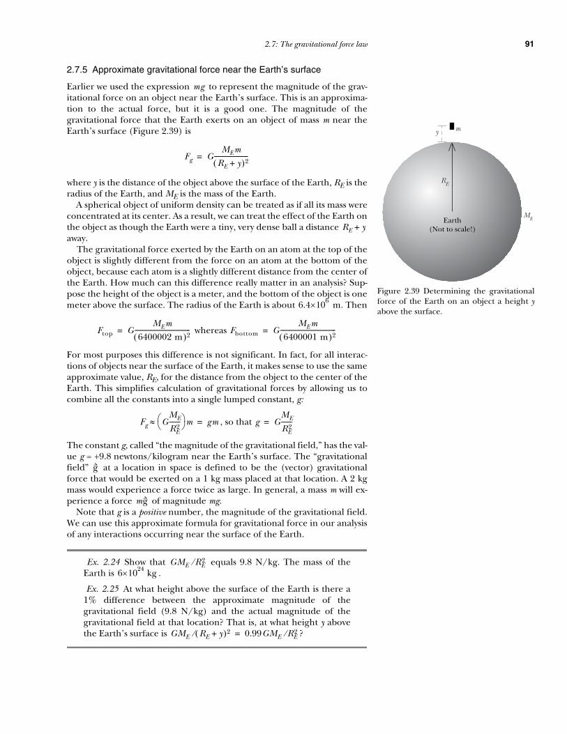
2.7: The gravitational force law 91
2.7.5 Approximate gravitational force near the Earth’s surface
Earlier we used the expression to represent the magnitude of the grav-itational force on an object near the Earth’s surface. This is an approxima-tion to the actual force, but it is a good one. The magnitude of thegravitational force that the Earth exerts on an object of mass m near theEarth’s surface (Figure 2.39) is
where y is the distance of the object above the surface of the Earth, RE is theradius of the Earth, and ME is the mass of the Earth.
A spherical object of uniform density can be treated as if all its mass wereconcentrated at its center. As a result, we can treat the effect of the Earth onthe object as though the Earth were a tiny, very dense ball a distance away.
The gravitational force exerted by the Earth on an atom at the top of theobject is slightly different from the force on an atom at the bottom of theobject, because each atom is a slightly different distance from the center ofthe Earth. How much can this difference really matter in an analysis? Sup-pose the height of the object is a meter, and the bottom of the object is onemeter above the surface. The radius of the Earth is about m. Then
whereas
For most purposes this difference is not significant. In fact, for all interac-tions of objects near the surface of the Earth, it makes sense to use the sameapproximate value, RE, for the distance from the object to the center of theEarth. This simplifies calculation of gravitational forces by allowing us tocombine all the constants into a single lumped constant, g:
, so that
The constant g, called “the magnitude of the gravitational field,” has the val-ue g = +9.8 newtons/kilogram near the Earth’s surface. The “gravitationalfield” at a location in space is defined to be the (vector) gravitationalforce that would be exerted on a 1 kg mass placed at that location. A 2 kgmass would experience a force twice as large. In general, a mass m will ex-perience a force of magnitude mg.
Note that g is a positive number, the magnitude of the gravitational field.We can use this approximate formula for gravitational force in our analysisof any interactions occurring near the surface of the Earth.
Ex. 2.24 Show that equals 9.8 N/kg. The mass of theEarth is .
Ex. 2.25 At what height above the surface of the Earth is there a1% difference between the approximate magnitude of thegravitational field (9.8 N/kg) and the actual magnitude of thegravitational field at that location? That is, at what height y abovethe Earth’s surface is ?
mg
Earth(Not to scale!)
y
RE
m
ME
Figure 2.39 Determining the gravitationalforce of the Earth on an object a height yabove the surface.
Fg GMEm
RE y+( )2----------------------=
RE y+
6.4 6×10
Ftop GMEm
6400002 m( )2------------------------------------= Fbottom G
MEm
6400001 m( )2------------------------------------=
Fg GME
RE2
-------⎝ ⎠⎛ ⎞ m≈ gm= g G
ME
RE2
-------=
g
mg
GME RE2⁄
6 24×10 kg
GME RE y+( )2⁄ 0.99GME RE2⁄=

92 Chapter 2: The Momentum Principle
2.8 The electric force law: Coulomb’s law
There are electric interactions between “charged” particles such as the pro-tons and electrons found in atoms. It is observed that two protons repel eachother, as do two electrons, while a proton and an electron attract each other(Figure 2.40; where protons are said to have “positive electric charge” andelectrons have “negative electric charge”).
The force corresponding to this electric interaction is similar to the grav-itational force law, and it is known as “Coulomb’s law” to honor the Frenchscientist who established this law in the late 1700’s, during the same periodwhen Cavendish measured the gravitational constant G. See Figure 2.41.
THE ELECTRIC FORCE LAW (COULOMB’S LAW)
where is a universal constant:
Both the gravitational and electric forces are proportional to the inversesquare of the center-to-center distance (“inverse square” laws). The univer-sal electric constant (read as “one over four pi epsilon-zero”) is very muchlarger than the gravitational constant, reflecting the fact that electric inter-actions are intrinsically much stronger than gravitational interactions. Forexample, consider a heavy weight that hangs from a thin metal wire. Thesmall number of atoms interacting electrically in the wire have as big an ef-fect on the hanging weight as a very much larger number of atoms in thehuge Earth, interacting gravitationally.
The charges q1 and q2 must be measured in SI units called “coulombs.”The proton has a charge of C and the electron has a charge of
.
? Study the three cases in Figure 2.40. Why is no minus sign neededin the force law, unlike the case with the gravitational force law?
The difference is that two positively charged particles such as two protonsrepel each other, whereas masses are always positive but the gravitationalforce is attractive. Two negatively charged particles such as electrons also at-tract each other and minus times minus gives plus. Only if the two particleshave opposite charges will they attract each other, and then the factor q2q1contributes the necessary minus sign, just as in the gravitational force law.
2.8.1 Interatomic forces
When two objects touch each other they exert forces on each other. At themicroscopic level, these contact forces are due to electric interactions be-tween the protons and electrons in one object and the protons and elec-trons in the other object. In Chapter 3 we will examine interatomic forcesin more detail.
Ex. 2.26 A proton and an electron are separated by , theradius of a typical atom. Calculate the magnitude of the electricforce that the proton exerts on the electron, and the magnitude ofthe electric force that the electron exerts on the proton.
Figure 2.40 Protons repel each other; elec-trons repel each other; protons and elec-trons attract each other.
Figure 2.41 The electric force exerted onobject 2 by object 1. (The force exerted onobject 2 by object 1 has the same magni-tude but opposite direction.)
q1
q2
Felec on 2 by 11
4πε0------------
q2q1
r2-12
------------- r̂2-1=
r2-1
r̂2-1Felec on 1 by 2
Felec on 2 by 11
4πε0------------
q2q1
r2-12
------------- r̂2-1=
14πε0------------ 1
4πε0------------ 9 9×10 N m2⋅
C2----------------=
+1.6 19–×101.6 19–×10–
1 10–×10 m
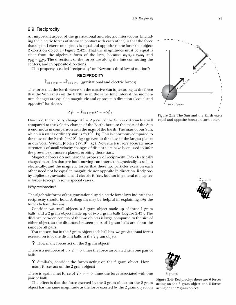
2.9: Reciprocity 93
2.9 Reciprocity
An important aspect of the gravitational and electric interactions (includ-ing the electric forces of atoms in contact with each other) is that the forcethat object 1 exerts on object 2 is equal and opposite to the force that object2 exerts on object 1 (Figure 2.42). That the magnitudes must be equal isclear from the algebraic form of the laws, because m1m2 = m2m1 andq1q2 = q2q1. The directions of the forces are along the line connecting thecenters, and in opposite directions.
This property is called “reciprocity” or “Newton’s third law of motion”:
RECIPROCITY
(gravitational and electric forces)
The force that the Earth exerts on the massive Sun is just as big as the forcethat the Sun exerts on the Earth, so in the same time interval the momen-tum changes are equal in magnitude and opposite in direction (“equal andopposite” for short):
However, the velocity change of the Sun is extremely smallcompared to the velocity change of the Earth, because the mass of the Sunis enormous in comparison with the mass of the Earth. The mass of our Sun,which is a rather ordinary star, is kg. This is enormous compared tothe mass of the Earth ( kg) or even to the mass of the largest planetin our Solar System, Jupiter ( kg). Nevertheless, very accurate mea-surements of small velocity changes of distant stars have been used to inferthe presence of unseen planets orbiting those stars.
Magnetic forces do not have the property of reciprocity. Two electricallycharged particles that are both moving can interact magnetically as well aselectrically, and the magnetic forces that these two particles exert on eachother need not be equal in magnitude nor opposite in direction. Reciproc-ity applies to gravitational and electric forces, but not in general to magnet-ic forces (except in some special cases).
Why reciprocity?
The algebraic forms of the gravitational and electric force laws indicate thatreciprocity should hold. A diagram may be helpful in explaining why theforces behave this way.
Consider two small objects, a 3 gram object made up of three 1 gramballs, and a 2 gram object made up of two 1 gram balls (Figure 2.43). Thedistance between centers of the two objects is large compared to the size ofeither object, so the distances between pairs of 1 gram balls are about thesame for all pairs.
You can see that in the 3 gram object each ball has two gravitational forcesexerted on it by the distant balls in the 2 gram object.
? How many forces act on the 3 gram object?
There is a net force of times the force associated with one pair ofballs.
? Similarly, consider the forces acting on the 2 gram object. Howmany forces act on the 2 gram object?
There is again a net force of times the force associated with onepair of balls.
The effect is that the force exerted by the 3 gram object on the 2 gramobject has the same magnitude as the force exerted by the 2 gram object on
y
x
z (out of page)
F on Ear
th by S
un
v
F on Sun by E
arth
Figure 2.42 The Sun and the Earth exertequal and opposite forces on each other.
Fon 1 by 2 Fon 2 by 1–=
∆p1 Fon 1 by 2∆t ∆p2–= =
∆v ∆p m⁄=
2 30×106 24×10
2 27×10
3 grams
2 grams
Figure 2.43 Reciprocity: there are 6 forcesacting on the 3 gram object and 6 forcesacting on the 2 gram object.
3 2× 6=
2 3× 6=

94 Chapter 2: The Momentum Principle
the 3 gram object. The same reciprocity holds, for the same reasons, for theelectric forces between a lithium nucleus containing 3 protons and a heliumnucleus containing 2 protons.
2.10 The Newtonian synthesis
Newton devised a particular explanatory scheme in which the analysis ofmotion is divided into two distinct parts:
1) Quantify the interaction in terms of a concept called “force.” Specificexamples are Newton’s law of gravitation and Coulomb’s law.
2) Quantify the change of motion in terms of the change in a quantitycalled “momentum.” The change in the momentum is equal to theforce times ∆t.
This scheme, called the “Newtonian synthesis,” has turned out to be extraor-dinarily successful in explaining a huge variety of diverse physical phenom-ena, from the fall of an apple to the orbiting of the Moon. Yet we have noway of asking whether the Universe “really” works this way. It seems unlikelythat the Universe actually uses the human concepts of “force” and “momen-tum” in the unfolding motion of an apple or the Moon.
We refer to the “Newtonian synthesis” both to identify and honor the par-ticular, highly successful analysis scheme introduced by Newton, but also toremind ourselves that this is not the only possible way to view and analyzethe universe.
Einstein’s alternative view
Newton stated his gravitational force law but could give no explanation forit. He was content with showing that it correctly predicted the motion of theplanets, and this was a huge advance, the real beginning of modern science.
Einstein made another huge advance by giving a deeper explanation forgravity, as a part of his general theory of relativity. He realized that the mas-sive Sun bends space and time (!) in such a way as to make the planets movethe way they do. The equations in Einstein’s general theory of relativitymake it possible to calculate the curvature of space and time due to massiveobjects, and to predict how other objects will move in this altered space andtime.
Moreover, Einstein’s theory of general relativity accurately predicts sometiny effects that Newton’s gravitational law does not, such as the slight bend-ing of light as it passes near the Sun. General relativity also explains somebizarre large-scale phenomena such as black holes and the observed expan-sion of the space between the galaxies.
Einstein’s earlier special theory of relativity established that nothing, noteven information, can travel faster than light. Because Newton’s gravitation-al force formula depends only on the distance between objects, not on thetime, something’s wrong with the formula, since this implies that if an objectwere suddenly yanked away, its force on another object would vanish instan-taneously, thus giving (in principle) a way to send information from oneplace to another instantaneously. Einstein’s theory of general relativitydoesn’t have this problem.
Since the equations of general relativity are very difficult to work with,and Newton’s gravitational law works very well for most purposes, in thiscourse we will use Newton’s approach to gravity. But you should be awarethat for the most precise calculations one must use the theory of general rel-ativity. For example, the highly accurate atomic clocks in the satellites thatmake up the Global Positioning System (GPS) have to be continually cor-rected using Einstein’s theory of general relativity. Otherwise GPS positionswould be wrong by several kilometers after just one day of operation!

2.11: *Derivation of special average velocity result 95
2.11 *Derivation of special average velocity result
Here we offer two proofs, one geometric and one algebraic (using calcu-lus), for the following special-case result concerning average velocity:
AVERAGE VELOCITY (SPECIAL CASE)
only if changes at a constant rate
( is constant, v << c); similar results for and
If is constant, implies that changes at a con-stant rate. At speeds small compared to the speed of light, , so agraph of vs. time is a straight line, as in Figure 2.44. In Figure 2.44 weform narrow vertical slices, each of height and narrow width .
Within each narrow slice changes very little, so the change in positionduring the brief time is approximately . Therefore thechange in x is approximately equal to the area of the slice of height andwidth (Figure 2.45).
If we add up the areas of all these slices, we get approximately the areaunder the line in Figure 2.44, and this is also equal to the total displacement
. If we go to the limit of an infinite number ofslices, each with infinitesimal width, the sum of slices really is the area, andthis area we have shown to be equal to the change in position. This kind ofsum of an infinite number of infinitesimal pieces is called an “integral” incalculus.
The area under the line is a trapezoid, and from geometry we know thatthe area of a trapezoid is the average of the two bases times the altitude.Turn Figure 2.44 on its side, as in Figure 2.46, and you see that the top andbottom have lengths and , while the altitude of the trapezoid is thetotal time . Therefore we have the following result:
Trapezoid area =
Dividing by , we have this:
But by definition the x component of average velocity is the change in x di-vided by the total time, so we have proved that
only if changes linearly with time ( is constant)
The proof depended critically on the straight-line (“linear”) change in ve-locity, which occurs only if is constant (and v << c). Otherwise wewouldn’t have a trapezoidal area. That’s why the result isn’t true in general;it’s only true in this important but special case.
Algebraic proof using calculus
An algebraic proof using calculus can also be given. We will use the x com-ponent of the derivative version of the Momentum Principle (more aboutthis in the next chapter):
implies that
vavg,xvxi vxf+( )
2------------------------= vx
Fnet,x vavg,y vavg,z
Fnet,x pxf pxi Fnet x, ∆t+= pxvx px m⁄≈
vx
t
vx
vx increases at constant rate
vxi
vxf
ti tf∆t ∆t∆t∆t∆t∆t∆t∆t∆t∆t ∆t
Figure 2.44 In this graph of vx vs. t (con-stant force), form narrow vertical sliceseach of height vx and width ∆t.
vx ∆tvx
∆t ∆x vx∆t=vx
∆t
vx
∆t
Figure 2.45 One narrow slice has an areagiven approximately by vx∆t. This is equalto ∆x, the displacement of the object.
Area vx∆t≈∆x1 ∆x2 ∆x3 ....+ + + xf xi–=
Figure 2.46 The area of the whole trape-zoid is equal to the total displacement.The figure in Figure 2.44 has been turnedon its side.
Bottom vxf=
Altitude tf ti–
Area Top Bottom+( )2
-----------------------------------------Altitude=
Top vxi=
vxi vxftf ti–( )
xf xi–vxi vxf+( )
2------------------------ tf ti–( )=
tf ti–( )
xf xi–
tf ti–--------------
vxi vxf+( )2
------------------------=
vavg,xvxi vxf+( )
2------------------------= vx Fnet,x
Fnet,x
∆p Fnet∆t= ∆p∆t------- Fnet=

96 Chapter 2: The Momentum Principle
In the limit we have and
If is a constant, the time derivative of is a constant, so we have
since when
You can check this by taking the derivative with respect to time t, which givesthe original equation . At speeds small compared to thespeed of light, , so we can write
since when
But the x component of velocity is the rate at which x is changing:
Now the question is, can you think of a function of x that has this time de-rivative? Since the time derivative of is , the following formula for x hasthe appropriate derivative:
since when
You can check this by taking the derivative with respect to t, which gives theequation for , since and .
The average velocity which we seek is the change in position divided bythe total time:
where we have used the equation we previously derived for the velocity:
Simplifying the expression for we have the proof:
only if changes at a constant rate ( is constant)
2.12 *Points and spheres
The gravitational force law applies to objects that are “point-like” (very smallcompared to the center-to-center distance between the objects). In the sec-ond volume of this textbook we will be able to show that any hollow spheri-cal shell with uniform density acts gravitationally on external objects asthough all the mass of the shell were concentrated at its center. The densityof the Earth is not uniform, because the central iron core has higher densitythan the outer layers. But by considering the Earth as layers of hollow spher-ical shells, like an onion, with each shell of nearly uniform density, we getthe result that the Earth can be modeled for most purposes as a point masslocated at the center of the Earth (for very accurate calculations one musttake into account small irregularities in the Earth’s density from place toplace). Similar statements can be made about other planets and stars. In Fig-ure 2.47, the gravitational force is correctly calculated using the center-to-center distance .
∆p∆t-------
∆ t 0→lim dp
dt------ Fnet= =
dpx
dt-------- Fnet,x=
Fnet,x px
px Fnet,xt pxi+= px pxi= t 0=
dpx dt⁄ Fnet,x=vx px m⁄≈
vxFnet,x
m------------t vxi+= vx vxi= t 0=
vxdxdt------
Fnet,x
m------------t vxi+= =
t2 2t
x 12---
Fnet,x
m------------t2 vxit xi+ += x xi= t 0=
vx d 12---t2( ) dt⁄ t= d t( ) dt⁄ 1=
vavg,xx xi–
t------------
12---
Fnet,x
m------------t vxi+
12--- vxf vxi–( ) vxi+= = =
vxf vxFnet,x
m------------t vxi+= =
vavg,x
vavg,xvxi vxf+( )
2------------------------= vx Fnet,x
m1m2
m1 m2
Equivalent:
Figure 2.47 A sphere whose densitydepends only on distance from the centeracts like a point particle with all the mass atthe center.
Fgrav Gm2m1
r2-12
--------------=
r2-1
r2-1

2.13: *Measuring the universal gravitational constant G 97
This is not an obvious result. After all, in Figure 2.47 some of the atomsare closer and some farther apart than the center-to-center distance ,but the net effect after adding up all the interactions of the individual atomsis as though the two objects had collapsed down to points at their centers.This is a very special property of forces, both gravitational and electric,and is not true for forces that have a different dependence on distance.
2.13 *Measuring the universal gravitational constant G
In order to make quantitative predictions and analyses of physical phenom-ena involving gravitational interactions, it is necessary to know the universalgravitational constant G. In 1797-1798 Henry Cavendish performed the firstexperiment to determine a precise value for G (Figure 2.48). In this kind ofexperiment, a bar with metal spheres at each end is suspended from a thinquartz fiber which constitutes a “torsional” spring. From other measure-ments, it is known how large a tangential force measured in newtons is re-quired to twist the fiber through a given angle. Large balls are brought nearthe suspended spheres, and one measures how much the fiber twists due tothe gravitational interactions between the large balls and the small spheres.
If the masses are measured in kilograms, the distance in meters, and theforce in newtons, the gravitational constant G has been measured in suchexperiments to be
This extremely small number reflects the fact that gravitational interactionsare inherently very weak compared with electromagnetic interactions. Theonly reason that gravitational interactions are significant in our daily lives isthat objects interact with the entire Earth, which has a huge mass. It takessensitive measurements such as the Cavendish experiment to observe grav-itational interactions between two ordinary-sized objects.
2.14 *The Momentum Principle is valid only in inertial frames
Newton’s first law is valid only in an “inertial frame” of reference, one in uni-form motion (or at rest) with respect to the pervasive “cosmic microwavebackground” (see optional discussion at the end of Chapter 1). Since theMomentum Principle is a quantitative version of Newton’s first law, we ex-pect the Momentum Principle to be valid in an inertial reference frame, butnot in a reference frame that is not in uniform motion. Let’s check that thisis true.
If you view some objects from a space ship that is moving uniformly withvelocity with respect to the cosmic microwave background, all of the ve-locities of those objects have the constant subtracted from them, as far asyou are concerned. For example, a rock moving at the same velocity as yourspacecraft would have in your reference frame: itwould appear to be stationary as it coasted along beside your spacecraft.
With a constant spaceship velocity, we have , and the change ofmomentum of the moving object reduces to the following (for speeds smallcompared to c):
since
Therefore,
r2-1
1 r2⁄
Figure 2.48 The Cavendish experiment.
G 6.7 11–×10 N m2⋅kg2
----------------=
vsvs
vrock v vs–( ) 0= =
∆vs 0=
∆ m v vs–( )[ ] ∆ mv( ) ∆ mvs( )– ∆ mv( )= = ∆ mvs( ) 0=
∆ m v vs–( )[ ] ∆ mv( ) Fnet∆t= =

98 Chapter 2: The Momentum Principle
If the velocity of the space ship doesn’t change (it represents an inertialframe of reference), the form (and validity) of the Momentum Principle isunaffected by the motion of the space ship.
However, if your space ship increases its speed, or changes direction,, an object’s motion relative to you changes without any force acting
on it. In that case the Momentum Principle is not valid for the object, be-cause you are not in an inertial frame. Although the Earth is not an inertialframe because it rotates, and goes around the Sun, it is close enough to be-ing an inertial frame for many everyday purposes.
2.15 *Updating position at high speed
If v << c, and . But at high speed it is more complicated todetermine the velocity from the (relativistic) momentum. Here is a way tosolve for in terms of :
Divide by m and square:
Multiply by :
Collect terms:
But since and are in the same direction, we can write this:
THE RELATIVISTIC POSITION UPDATE FORMULA
(for small )
Note that at low speeds , and the denominator is ,so the formula becomes the familiar .
2.16 *Definitions, measurements, and units
Using the Momentum Principle requires a consistent way to measurelength, time, mass, and force, and a consistent set of units. We state the def-initions of the standard Système Internationale (SI) units, and we briefly dis-cuss some subtle issues underlying this choice of units.
Units: meters, seconds, kilograms, and newtons
Originally the meter was defined as the distance between two scratches on aplatinum bar in a vault in Paris, and a second was 1/86,400th of a “mean so-
vs
∆vs 0≠
p mv≈ v p m⁄≈
v p
p 1
1 v c⁄( )2–--------------------------------m v=
p 2
m2-------- v 2
1 v c⁄( )2–----------------------------=
1 v c⁄( )2–( ) p 2
m2--------
p 2
m2c2-----------⎝ ⎠
⎛ ⎞ v 2– v 2=
1 p 2
m2c2-----------+⎝ ⎠
⎛ ⎞ v 2 p 2
m2--------=
v p m⁄
1p
mc------⎝ ⎠
⎛ ⎞2
+
----------------------------=
p v
v p m⁄
1p
mc------⎝ ⎠
⎛ ⎞2
+
----------------------------=
rf ri1
1p
mc------⎝ ⎠
⎛ ⎞2
+
---------------------------- pm----⎝ ⎠
⎛ ⎞ ∆t+= ∆t
p m v≈ 1 vc
-----⎝ ⎠⎛ ⎞
2+ 1≈
rf ri p m⁄( )∆t+=

2.16: *Definitions, measurements, and units 99
lar day.” Now however the second is defined in terms of the frequency oflight emitted by a cesium atom, and the meter is defined as the distancelight travels in 1/299,792,458th of a second, or about seconds (3.3nanoseconds). The speed of light is defined to be exactly 299,792,458 m/s(very close to m/s). As a result of these modern redefinitions, it is re-ally speed (of light) and time that are the internationally agreed-upon basicunits, not length and time.
By international agreement, one kilogram is the mass of a platinum blockkept in that same vault in Paris. As a practical matter, other masses are com-pared to this standard kilogram by using a balance-beam or spring weighingscale (more about this in a moment). The newton, the unit of force, is de-fined as that force which acting for 1 second imparts to 1 kilogram a velocitychange of 1 m/s. We could make a scale for force by calibrating the amountof stretch of a spring in terms of newtons.
Some subtle issues
What we have just said about SI units is sufficient for practical purposes topredict the motion of objects, but here are some questions that might both-er you. Is it legitimate to measure the mass that appears in the MomentumPrinciple by seeing how that mass is affected by gravity on a balance-beamscale? Is it legitimate to use the Momentum Principle to define the units offorce, when the concept of force is itself associated with the same law? Is thisall circular reasoning, and the Momentum Principle merely a definitionwith little content? Here is a chain of reasoning that addresses these issues.
Measuring inertial mass
When we use balance-beam or spring weighing scales to measure mass, whatwe’re really measuring is the “gravitational mass,” that is, the mass that ap-pears in the law of gravitation and is a measure of how much this object isaffected by the gravity of the Earth. In principle, it could be that this “grav-itational mass” would be different from the so-called “inertial mass”—themass that appears in the definition of momentum. It is possible to comparethe inertial masses of two objects, and we find experimentally that inertialand gravitational mass seem to be entirely equivalent.
Here is a way to compare two inertial masses directly, without involvinggravity. Starting from rest, pull on the first object with a spring stretched bysome amount s for an amount of time ∆t, and measure the increase of speed
. Then, starting from rest, pull on the second object with the samespring stretched by the same amount s for the same amount of time ∆t, andmeasure the increase of speed . We define the ratio of the inertial mass-es as . Since one of these masses could be the standardkilogram kept in Paris, we now have a way of measuring inertial mass in ki-lograms. Having defined inertial mass this way, we find experimentally thatthe Momentum Principle is obeyed by both of these objects in all situations,not just in the one special experiment we used to compare the two masses.
Moreover, we find to extremely high precision that the inertial mass in ki-lograms measured by this comparison experiment is exactly the same as thegravitational mass in kilograms obtained by comparing with a standard kilo-gram on a balance-beam scale (or using a calibrated spring scale), and thatit doesn’t matter what the objects are made of (wood, copper, glass, etc.).This justifies the convenient use of ordinary weighing scales to determineinertial mass.
Is this circular reasoning?
The definitions of force and mass may sound like circular reasoning, andthe Momentum Principle may sound like just a kind of definition, with no
3.3 9–×10
3 8×10
∆v1
∆v2m1 m2⁄ ∆v2 ∆v1⁄=

100 Chapter 2: The Momentum Principle
real content, but there is real power in the Momentum Principle. Forget fora moment the definition of force in newtons and mass in kilograms. The ex-perimental fact remains that any object if subjected to a single force by aspring with constant stretch experiences a change of momentum (and ve-locity) proportional to the duration of the interaction. Note that it is not achange of position proportional to the time (that would be a constantspeed), but a change of velocity. That’s real content. Moreover, we find thatthe change of velocity is proportional to the amount of stretch of the spring.That too is real content.
Then we find that a different object undergoes a different rate of changeof velocity with the same spring stretch, but after we’ve made one singlecomparison experiment to determine the mass relative to the standard kilo-gram, the Momentum Principle works in all situations. That’s real content.
Finally come the details of setting standards for measuring force in new-tons and mass in kilograms, and we use the Momentum Principle in helpingset these standards. But logically this comes after having established the lawitself.

2.17: Summary 101
2.17 Summary
Fundamental Physical Principles
THE MOMENTUM PRINCIPLE
(for a short enough time interval ∆t)
Update form:
THE SUPERPOSITION PRINCIPLE
The net force on an object is the vector sum of the individual forces exertedon it by all other objects. Each individual interaction is unaffected by thepresence of other interacting objects.
Major new concepts
To apply the Momentum Principle to analyze the motion of a real-world sys-tem, several steps are required:
1. Choose a system, consisting of a portion of the Universe.The rest of the Universe is called the surroundings.
2. List objects in the surroundings that exert significant forces on the chosen system, and make a labeled diagram showing the external forcesexerted by the objects in the surroundings.
3. Apply the Momentum Principle to the chosen system:
For each term in the Momentum Principle, substitute any values you know.
4. Apply the position update formula, if necessary:
5. Solve for any remaining unknown quantities of interest.
6. Check for reasonableness (units, etc.).
System is a portion of the Universe acted on by the surroundings.
Force is a quantitative measure of interactions; units are newtons.
Impulse is the product of force times time ; momentum change equalsnet impulse (the impulse due to the net force).
Four fundamental types of interaction have been identified:• gravitational interactions (all objects attract each other gravitational-
ly)• electromagnetic interactions (electric and magnetic interactions,
closely related to each other); interatomic forces are electric in nature• “strong” interactions (inside the nucleus of an atom)• “weak” interactions (neutron decay, for example)
Physical models are tractable approximations/idealizations of the real world.
∆p Fnet∆t=
pf pi Fnet∆t+=
A labeled diagram (step 3) gives a physicsview of the situation, and it defines sym-bols to use in writing an algebraic state-ment of the Momentum Principle.
pf pi Fnet∆t+=
rf ri varg∆t+=
F∆t

102 Chapter 2: The Momentum Principle
Computer prediction of motion:
Force laws
THE GRAVITATIONAL FORCE LAW
points from the center of object 1 to the center of object 2
G is a universal constant:
Near the Earth’s surface, , where g = +9.8 N/kg
THE ELECTRIC FORCE LAW (COULOMB’S LAW)
where is a universal constant:
THE SPRING FORCE LAW (MAGNITUDE)
s is the stretch: (relaxed length - new length)
is called the “spring stiffness”
RECIPROCITY
(gravitational and electric forces)
This is also called “Newton’s third law of motion.”
Additional new concepts and results
Uniform-density spheres act as though all the mass were at the center.
AVERAGE VELOCITY (SPECIAL CASE)
exactly true only if v << c and changes at a constant rate ( constant)
• Define the values of constants such as G to use in the program.• Specify the masses, initial positions, and initial momenta of the inter-
acting objects.• Specify an appropriate value for , small enough that the objects
don’t move very far during one update.• Create a “loop” structure for repetitive calculations:
• Calculate the (vector) forces acting on each object.• Update the momentum of each object: .• Update the positions: , where .• Repeat.
∆t
pf pi Fnet∆t+=rf ri varg∆t+= varg pf m⁄≈
m1
m2
Fgrav on 1 by 2
Figure 2.49 The gravitational force exertedon object 2 by object 1. (The force exertedon object 1 by object 2 has the same magni-tude but opposite direction.)
r2-1
Fgrav on 2 by 1 G–m2m1
r2-12
-------------- r̂2-1=
r̂2-1
Fgrav on 2 by 1 G–m2m1
r2-12
------------- r̂2-1=
r2-1
G 6.7 11–×10 N m2⋅kg2
----------------=
Fgrav mg=
Figure 2.50 The electric force exerted onobject 2 by object 1. (The force exerted onobject 2 by object 1 has the same magni-tude but opposite direction.)
q1
q2
Felec on 2 by 11
4πε0------------
q2q1
r2-12
------------- r̂2-1=
r2-1
r̂2-1Felec on 1 by 2
Felec on 2 by 11
4πε0------------
q2q1
r2-12
------------- r̂2-1=
14πε0------------ 1
4πε0------------ 9 9×10 N m2⋅
C2----------------=
Fspring ks s=
s ∆L L L0–= =
ks
Fon 1 by 2 Fon 2 by 1–=
vavgvi vf+( )
2-------------------≈
v Fnet

2.18: Review questions 103
2.18 Review questions
The Momentum Principle
RQ 2.1 At a certain instant, a particle is moving in the +x direction with mo-mentum +10 kg·m/s. During the next 0.1 s, a constant force acts on the par-ticle: Fx = –6 N, and Fy = +3 N. What is the magnitude of the momentum ofthe particle at the end of this 0.1 s interval?
RQ 2.2 At t = 12.0 seconds an object with mass 2 kg was observed to have avelocity of <10, 35, –8> m/s. At t = 12.3 seconds its velocity was <20, 30, 4>m/s. What was the average (vector) net force acting on the object?
RQ 2.3 A proton has mass . What is the magnitude of the im-pulse required to increase its speed from 0.990c to 0.994c?
The gravitational force law
RQ 2.4 Calculate the approximate gravitational force exerted by the Earthon a human standing on the Earth’s surface. Compare with the approxi-mate gravitational force of a human on another human at a distance of 3meters. What approximations or simplifying assumptions must you make?(See data on the inside back cover.)
Reciprocity
RQ 2.5 The windshield of a speeding car hits a hovering insect. Comparethe magnitude of the force that the car exerts on the bug to the force thatthe bug exerts on the car. Which is bigger? Compare the magnitude of thechange of momentum of the bug to that of the car. Which is bigger? Com-pare the magnitude of the change of velocity of the bug to that of the car.Which is bigger? Explain briefly. (Note: the interatomic forces between bugand windshield are electric forces.)
The superposition principle
RQ 2.6 In order to pull a sled across a level field at constant velocity youhave to exert a constant force. Doesn’t this violate Newton’s first and secondlaws of motion, which imply that no force is required to maintain a constantvelocity? Explain this seeming contradiction.
1.7 27–×10 kg

104 Chapter 2: The Momentum Principle
2.19 Problems
Problem 2.1 In the space shuttleA space shuttle is in a circular orbit near the Earth. An astronaut floats inthe middle of the shuttle, not touching the walls. On a diagram, draw andlabel
(a) the momentum of the astronaut at this instant; (b) all of the forces (if any) acting on the astronaut at this instant; (c) the momentum of the astronaut a short time ∆t later; (d) the momentum change (if any) in this time interval. (e) Why does the astronaut seem to “float” in the shuttle?
It is ironic that we say the astronaut is “weightless” despite the fact that theonly force acting on the astronaut is the astronaut’s weight (that is, the grav-itational force of the Earth on the astronaut).
Problem 2.2 Two books attract each otherTwo copies of this textbook are standing right next to each other on a book-shelf. Make a rough estimate of the magnitude of the gravitational force thatthe books exert on each other. Explicitly list all quantities that you had toestimate, and all simplifications and approximations you had to make to dothis calculation. Compare your result to the gravitational force on the bookby the Earth.
Problem 2.3 Compare gravitational and electric forcesUse data from the inside back cover to calculate the gravitational and elec-tric forces two protons exert on each other when they are apart(about one atomic radius). Which interaction between two protons is stron-ger, the gravitational attraction or the electric repulsion? If the two protonsare at rest, will they begin to move toward each other or away from each oth-er? Note that since both the gravitational and electric force laws depend onthe inverse square distance, this comparison holds true at all distances, notjust at a distance of .
Problem 2.4 Crash testIn a crash test, a truck with mass 2200 kg traveling at 25 m/s (about 55 milesper hour) smashes head-on into a concrete wall without rebounding. Thefront end crumples so much that the truck is 0.8 m shorter than before.What is the approximate magnitude of the force exerted on the truck by thewall? Explain your analysis carefully, and justify your estimates on physicalgrounds.
Problem 2.5 Ping-pong ballA ping-pong ball is acted upon by the Earth, air resistance, and a strongwind. Here are the positions of the ball at several times.
Early time interval:At t = 12.35 s, the position was < 3.17, 2.54, –9.38 > mAt t = 12.37 s, the position was < 3.25, 2.50, –9.40 > m
Late time interval:At t = 14.35 s, the position was < 11.25, –1.50, –11.40 > mAt t = 14.37 s, the position was < 11.27, –1.86, –11.42 > m
(a) In the early time interval, from t = 12.35 s to t = 12.37 s, what was theaverage momentum of the ball? The mass of the ping-pong ball is 2.7 grams( kg). Express your result as a vector.
(b) In the late time interval, from t = 14.35 s to t = 14.37 s, what was theaverage momentum of the ball? Express your result as a vector.
(c) In the time interval from t = 12.35 s (the start of the early time inter-val) to t = 14.35 s (the start of the late time interval), what was the averagenet force acting on the ball? Express your result as a vector.
p1
p2∆p
1 10–×10 m
1 10–×10 m
2.7 3–×10

2.19: Problems 105
Problem 2.6 Kick a basketballA 0.6 kg basketball is rolling by you at 3.5 m/s. As it goes by, you give it akick perpendicular to its path (Figure 2.51). Your foot is in contact with theball for 0.002 s. The ball eventually rolls at a 20º angle from its original di-rection. The overhead view is approximately to scale. The arrow representsthe force your toe applies briefly to the basketball.
(a) In the diagram, which letter corresponds to the correct overhead viewof the ball’s path?
(b) Determine the magnitude of the average force you applied to theball.
Problem 2.7 Spacecraft and asteroidAt t = 532.0 s after midnight a spacecraft of mass 1400 kg is located at posi-tion , and an asteroid of mass is locat-ed at position . There are no other objectsnearby.
(a) Calculate the (vector) force acting on the spacecraft.(b) At the spacecraft’s momentum was , and at the later
time its momentum was , Calculate the (vector) change ofmomentum .
Problem 2.8 Proton and HCl moleculeA proton interacts electrically with a neutral HCl molecule located at the or-igin. At a certain time t, the proton’s position is and theproton’s velocity is . The force exerted on the proton bythe HCl molecule is . At a time , what isthe approximate velocity of the proton?
Problem 2.9 A free throw in basketballDetermine two different possible ways for a player to make a free throw inbasketball. In both cases give the initial speed, initial angle, and initialheight of the basketball. The rim of the basket is 10 feet (3.0 m) above thefloor. It is 14 feet (4.3 m) along the floor from the free-throw line to a pointdirectly below the center of the basket.
Problem 2.10 A basketball passYou have probably seen a basketball player throw the ball to a teammate atthe other end of the court, 30 m away. Estimate a reasonable initial anglefor such a throw, and then determine the corresponding initial speed. Foryour chosen angle, how long does it take for the basketball to go the lengthof the court? What is the highest point along the trajectory, relative to thethrower’s hand?
Problem 2.11 The case of the falling flower potYou are a detective investigating why someone was hit on the head by a fall-ing flowerpot. One piece of evidence is a home video taken in a 4th-floorapartment, which happens to show the flowerpot falling past a tall window.Inspection of individual frames of the video shows that in a span of 6 framesthe flowerpot falls a distance that corresponds to 0.85 of the window heightseen in the video (note: standard video runs at a rate of 30 frames per sec-ond). You visit the apartment and measure the window to be 2.2 m high.What can you conclude? Under what assumptions? Give as much detail asyou can.
Problem 2.12 Tennis ball hits wallA tennis ball has a mass of 0.057 kg. A professional tennis player hits the ballhard enough to give it a speed of 50 m/s (about 120 miles per hour). Theball hits a wall and bounces back with almost the same speed (50 m/s). Asindicated in Figure 2.52, high-speed photography shows that the ball is
20˚
20˚
20˚
A
C
B
Figure 2.51 Kick a basketball (Problem2.6).
3 5×10 7 5×10 4 5×10–, ,⟨ ⟩ m 7 15×10 kg9 5×10 3– 5×10 12 5×10–, ,⟨ ⟩ m
t 532.0 s= pit 538.0 s= pf
pf pi–
1.6 9–×10 0 0, ,⟨ ⟩ m3200 800 0, ,⟨ ⟩ m/s
1.12– 11–×10 0 0, ,⟨ ⟩ N t 2 14–×10 s( )+
2 cm
Figure 2.52 A high-speed tennis balldeforms when it hits a wall (Problem 2.12).

106 Chapter 2: The Momentum Principle
crushed 2 cm (0.02 m) at the instant when its speed is momentarily zero, be-fore rebounding.
Making the very rough approximation that the large force that the wallexerts on the ball is approximately constant during contact, determine theapproximate magnitude of this force. Hint: Think about the approximateamount of time it takes for the ball to come momentarily to rest. (For com-parison note that the gravitational force on the ball is quite small, only about
. A force of 5 N force is approximately the sameas a force of one pound.)
Problem 2.13 Mars probeA small space probe, of mass 240 kg, is launched from a spacecraft nearMars. It travels toward the surface of Mars, where it will land. At a time 20.7seconds after it is launched, the probe is at the location
, and at this same time its momentum is. At this instant, the net force on the
probe due to the gravitational pull of Mars plus the air resistance acting onthe probe is .
(a) Assuming that the net force on the probe is approximately constantover this time interval, what is the momentum of the probe 20.9 seconds af-ter it is launched?
(b,) What is the location of the probe 20.9 seconds after launch?
Problem 2.14 Spacecraft navigationSuppose you are navigating a spacecraft far from other objects. The mass ofthe spacecraft is (about 150 tons). The rocket engines are shutoff, and you’re coasting along with a constant velocity of . Asyou pass the location you briefly fire side thruster rockets, sothat your spacecraft experiences a net force of for 3.4 s. Theejected gases have a mass that is small compared to the mass of the space-craft. You then continue coasting with the rocket engines turned off. Whereare you an hour later? Also, what approximations or simplifying assump-tions did you have to make in your analysis? Think about the choice of sys-tem: what are the surroundings that exert external forces on your system?
Problem 2.15 Electron motion in a CRTIn a cathode ray tube (CRT) used in oscilloscopes and televi-sion sets, a beam of electrons is steered to different places on aphosphor screen, which glows at locations hit by electrons (Fig-ure 2.53). The CRT is evacuated, so there are few gas moleculespresent for the electrons to run into. Electric forces are used toaccelerate electrons of mass m to a speed v0 << c, after whichthey pass between positively and negatively charged metalplates which deflect the electron in the vertical direction (up-ward in Figure 2.53, or downward if the sign of the charges onthe plates is reversed). While an electron is between the plates, it experiences a uni-form vertical force F, but when the electron is outside the platesthere is negligible force on it. The gravitational force on theelectron is negligibly small compared to the electric force inthis situation. The length of the metal plates is d, and the phos-phor screen is a distance L from the metal plates. Where doesthe electron hit the screen? (That is, what is yf?)
0.057 kg( ) 9.8 N/kg( ) 0.6 N≈
4.30 3×10 8.70 2×10 0, ,⟨ ⟩ m4.40 4×10 7.60– 3×10 0, ,⟨ ⟩ kg m⋅ s⁄
7– 3×10 9.2– 2×10 0, ,⟨ ⟩ N
1.5 5×10 kg0 20 0, ,⟨ ⟩ km/s
12 15 0, ,⟨ ⟩ km6 4×10 0 0, ,⟨ ⟩ N
+ + + + + + + + +
– – – – – – – – –
d L
yf = ?
v0
e–
Figure 2.53 A cathode ray tube (Problem2.15).
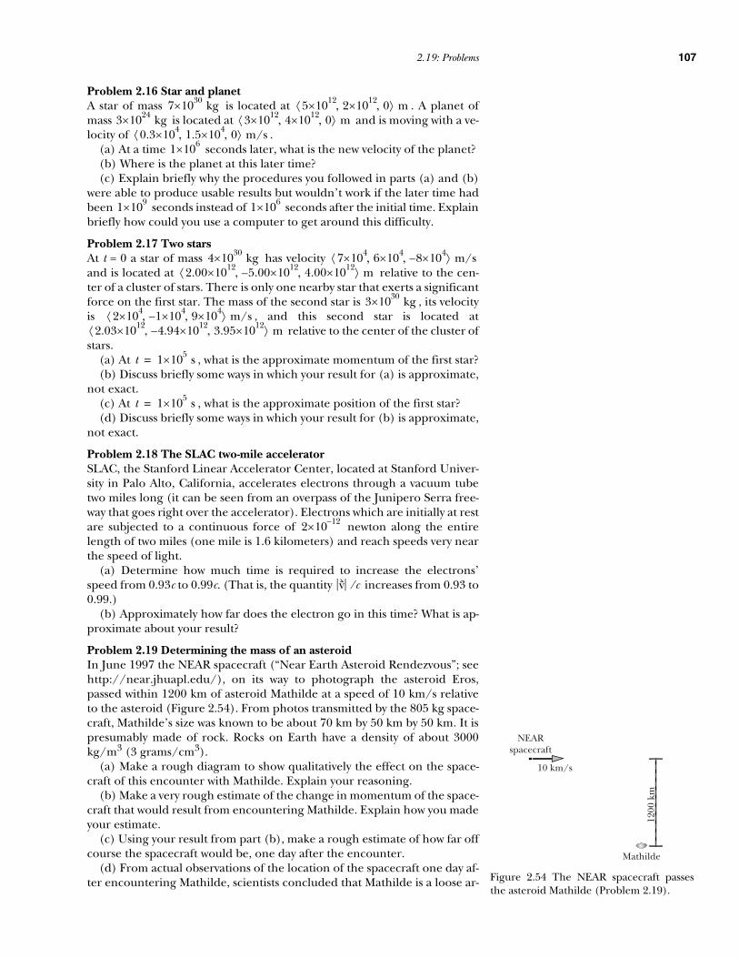
2.19: Problems 107
Problem 2.16 Star and planetA star of mass is located at . A planet ofmass is located at and is moving with a ve-locity of .
(a) At a time seconds later, what is the new velocity of the planet? (b) Where is the planet at this later time?(c) Explain briefly why the procedures you followed in parts (a) and (b)
were able to produce usable results but wouldn’t work if the later time hadbeen seconds instead of seconds after the initial time. Explainbriefly how could you use a computer to get around this difficulty.
Problem 2.17 Two starsAt t = 0 a star of mass has velocity and is located at relative to the cen-ter of a cluster of stars. There is only one nearby star that exerts a significantforce on the first star. The mass of the second star is , its velocityis , and this second star is located at
relative to the center of the cluster ofstars.
(a) At , what is the approximate momentum of the first star?(b) Discuss briefly some ways in which your result for (a) is approximate,
not exact.(c) At , what is the approximate position of the first star?(d) Discuss briefly some ways in which your result for (b) is approximate,
not exact.
Problem 2.18 The SLAC two-mile acceleratorSLAC, the Stanford Linear Accelerator Center, located at Stanford Univer-sity in Palo Alto, California, accelerates electrons through a vacuum tubetwo miles long (it can be seen from an overpass of the Junipero Serra free-way that goes right over the accelerator). Electrons which are initially at restare subjected to a continuous force of newton along the entirelength of two miles (one mile is 1.6 kilometers) and reach speeds very nearthe speed of light.
(a) Determine how much time is required to increase the electrons’speed from 0.93c to 0.99c. (That is, the quantity increases from 0.93 to0.99.)
(b) Approximately how far does the electron go in this time? What is ap-proximate about your result?
Problem 2.19 Determining the mass of an asteroidIn June 1997 the NEAR spacecraft (“Near Earth Asteroid Rendezvous”; seehttp://near.jhuapl.edu/), on its way to photograph the asteroid Eros,passed within 1200 km of asteroid Mathilde at a speed of 10 km/s relativeto the asteroid (Figure 2.54). From photos transmitted by the 805 kg space-craft, Mathilde’s size was known to be about 70 km by 50 km by 50 km. It ispresumably made of rock. Rocks on Earth have a density of about 3000kg/m3 (3 grams/cm3).
(a) Make a rough diagram to show qualitatively the effect on the space-craft of this encounter with Mathilde. Explain your reasoning.
(b) Make a very rough estimate of the change in momentum of the space-craft that would result from encountering Mathilde. Explain how you madeyour estimate.
(c) Using your result from part (b), make a rough estimate of how far offcourse the spacecraft would be, one day after the encounter.
(d) From actual observations of the location of the spacecraft one day af-ter encountering Mathilde, scientists concluded that Mathilde is a loose ar-
7 30×10 kg 5 12×10 2 12×10 0, ,⟨ ⟩ m3 24×10 kg 3 12×10 4 12×10 0, ,⟨ ⟩ m
0.3 4×10 1.5 4×10 0, ,⟨ ⟩ m/s1 6×10
1 9×10 1 6×10
4 30×10 kg 7 4×10 6 4×10 8 4×10–, ,⟨ ⟩ m/s2.00 12×10 5.00 12×10– 4.00 12×10, ,⟨ ⟩ m
3 30×10 kg2 4×10 1 4×10– 9 4×10, ,⟨ ⟩ m/s
2.03 12×10 4.94 12×10– 3.95 12×10, ,⟨ ⟩ m
t 1 5×10 s=
t 1 5×10 s=
2 12–×10
v c⁄
Mathilde
1200
km
NEARspacecraft
10 km/s
Figure 2.54 The NEAR spacecraft passesthe asteroid Mathilde (Problem 2.19).

108 Chapter 2: The Momentum Principle
rangement of rocks, with lots of empty space inside. What was it about theobservations that must have led them to this conclusion?
Experimental background: The position was tracked by very accuratemeasurements of the time that it takes for a radio signal to go from Earth tothe spacecraft followed immediately by a radio response from the spacecraftbeing sent back to Earth. Radio signals, like light, travel at a speed of m/s, so the time measurements had to be accurate to a few nanoseconds( ).
The following problems are intended to introduce you to using a computerto model matter, interactions, and motion. Some parts of these problemscan be done with almost any tool (spreadsheet, math package, etc.). Otherparts are most easily done with a programming language, for which we rec-ommend the free 3D programming language VPython (http://vpy-thon.org). Your instructor will introduce you to an available computationaltool and assign problems, or parts of problems, that can be addressed usingthe chosen tool.
Problem 2.20 Planetary orbitsIn this problem you will study the motion of a planet around a star. To startwith a somewhat familiar situation, you will begin by modeling the motionof our Earth around our Sun. Write answers to questions either as com-ments in your program or on paper, as specified by your instructor.
Planning(a) The Earth goes around the Sun in a nearly circular orbit, taking one
year to go around. Using data on the inside back cover, what initial speedshould you give the Earth in a computer model, so that a circular orbitshould result? (If your computer model does produce a circular orbit, youhave a strong indication that your program is working properly.)
(b) Estimate an appropriate value for ∆t to use in your computer model.Remember that t is in seconds, and consider your answer to part (a) in mak-ing this estimate. If your ∆t is too small, your calculation will require manytedious steps. Explain briefly how you decided on an appropriate step size.
Circular orbit(c) Starting with speed calculated in (a), and with the initial velocity per-
pendicular to a line connecting the Sun and the Earth, calculate and displaythe trajectory of the Earth. Display the whole trail, so you can see whetheryou have a closed orbit (that is, whether the Earth returns to its startingpoint each time around). Include the Sun’s position in yourcomputations, even if you set its coordinates to zero. This will make it easierto modify the computation to let the Sun move (Problem 2.2 Binary stars).
Computational accuracy(d) As a check on your computation, is the orbit a circle as expected? Run
the calculation until the accumulated time t is the length of a year: does thistake the Earth around the orbit once, as expected? What is the largest stepsize you can use that still gives a circular orbit and the correct length of ayear? What happens if you use a much larger step size?
Noncircular trajectories(e) Set the initial speed to 1.2 times the Earth’s actual speed. Make sure
the step size is small enough that the orbit is nearly unaffected if you cut thestep size. What kind of orbit do you get? What step size do you need to useto get results you can trust? What happens if you use a much larger step size?Produce at least one other qualitatively different noncircular trajectory for
3 8×10
1 ns 10 9– s=
rs <xs ys zs, , >=

2.19: Problems 109
the Earth. What difficulties would humans have in surviving on the Earth ifit had a highly noncircular orbit?
Force and momentum(f) Choose initial conditions that give a noncircular orbit. Continuously
display a vector showing the momentum of the Earth (with its tail at theEarth’s position), and a different colored vector showing the force on theEarth by the Sun (with its tail at the Earth’s position). You must scale thevectors appropriately to fit into the scene. A way to figure out what scale fac-tor to use is to print the numerical values of momentum and force, andcompare with the scale of the scene. For example, if the width of the sceneis W meters, and the force vector has a typical magnitude F (in newtons),you might scale the force vector by a factor 0.1W/F, which would make thelength of the vector be one-tenth the width of the scene. Is the force in thesame direction as the momentum? How does the momentum depend onthe distance from the star?
Problem 2.21 Binary starsAbout a half of the visible “stars” are actually systems consisting of two starsorbiting each other, called “binary stars.” In your computer model of theEarth and Sun (Problem 2.20 Planetary orbits ), replace the Earth with astar whose mass is half the mass of our Sun, and take into account the grav-itational effects that the second star has on the Sun.
(a) Give the second star the speed of the actual Earth, and give the Sunzero initial momentum. What happens? Try a variety of other initial condi-tions. What kinds of orbits do you find?
(b) One of the things to try is to give the Sun the same magnitude of mo-mentum as the second star, but in the opposite direction. If the initial mo-mentum of the second star is in the +y direction, give the Sun the samemagnitude of momentum but in the –y direction, so that the total momen-tum of the binary star system is initially zero, but the stars are not headedtoward each other. What is special about the motion you observe in thiscase?
Problem 2.22 Other force lawsModify your orbit computation to use a different force law, such as a forcethat is proportional to or , or a constant force, or a force propor-tional to (this represents the force of a spring whose relaxed length isnearly zero). How do orbits with these force laws differ from the circles andellipses that result from a law? If you want to keep the magnitude ofthe force roughly the same as before, you will need to adjust the force con-stant G.
Problem 2.23 The effect of the Moon and Venus on the EarthIn Problem 2.20 you analyzed a simple model of the Earth orbiting the Sun,in which there were no other planets or moons. Venus and the Earth havesimilar size and mass. At its closest approach to the Earth, Venus is about 40million kilometers away ( m). The Moon’s mass is about kg,and the distance from Earth to Moon is about m (400,000 km, centerto center).
(a) Calculate the ratio of the gravitational forces on the Earth exerted byVenus and the Sun. Is it a good approximation to ignore the effect of Venuswhen modeling the motion of the Earth around the Sun?
(b) Calculate the ratio of the gravitational forces on the Earth exerted bythe Moon and the Sun. Is it a good approximation to ignore the effect ofthe Moon when modeling the motion of the Earth around the Sun?
1 r⁄ 1 r⁄ 3
r2
1 r⁄ 2
4 10×10 7 22×104 8×10

110 Chapter 2: The Momentum Principle
Problem 2.24 The three-body problemCarry out a numerical integration of the motion of a three-body gravitation-al system and plot the trajectory, leaving trails behind the objects. Calculateall of the forces before using these forces to update the momenta and posi-tions of the objects. Otherwise the calculations of gravitational forces wouldmix positions corresponding to different times.
Try different initial positions and initial momenta. Find at least one set ofinitial conditions that produces a long-lasting orbit, one set of initial condi-tions that results in a collision with a massive object, and one set of initialconditions that allows one of the objects to wander off without returning.Report the masses and initial conditions that you used.
Problem 2.25 The Ranger 7 mission to the MoonThe first U.S. spacecraft to photographthe Moon close up was the unmanned“Ranger 7” photographic mission in1964. The spacecraft, shown in the illus-tration at the right (NASA photograph),contained television cameras that trans-mitted close-up pictures of the Moonback to Earth as the spacecraft ap-proached the Moon. The spacecraft didnot have retro-rockets to slow itself down,and it eventually simply crashed onto theMoon’s surface, transmitting its last pho-tos immediately before impact.
Figure 2.55 is the first image of the Moon taken by a U.S. spacecraft, Rang-er 7, on July 31, 1964, about 17 minutes before impacting the lunar surface.The large crater at center right is Alphonsus (108 km diameter); above it(and to the right) is Ptolemaeus and below it is Arzachel. The Ranger 7 im-pact site is off the frame, to the left of the upper left corner.
You can find out more about the actual Ranger lunar missions athttp://nssdc.gsfc.nasa.gov/planetary/lunar/ranger.html
To send a spacecraft to the Moon, we put it on top of a large rocket contain-ing lots of rocket fuel and fire it upward. At first the huge ship moves quiteslowly, but the speed increases rapidly. When the “first-stage” portion of therocket has exhausted its fuel and is empty, it is discarded and falls back toEarth. By discarding an empty rocket stage we decrease the amount of massthat must be accelerated to even higher speeds. There may be several stagesthat operate for a while and then are discarded before the spacecraft has ris-en above most of Earth’s atmosphere (about 50 km, say, above the Earth),and has acquired a high speed. At that point all the fuel available for thismission has been used up, and the spacecraft simply coasts toward the Moonthrough the vacuum of space.
We will model the Ranger 7 mission. Starting 50 km above the Earth’s sur-face ( m), a spacecraft coasts toward the Moon with an initial speed ofabout 104 m/s. Here are data we will need:
mass of spacecraft = 173 kg mass of Earth ≈ kg
mass of Moon ≈ kg radius of Moon = mdistance from Earth to Moon ≈ m (400,000 km, center to center)
We’re going to ignore the Sun in a simplified model even though it exertsa sizable gravitational force. We’re expecting the Moon mission to take onlya few days, during which time the Earth (and Moon) move in a nearlystraight line with respect to the Sun, because it takes 365 days to go all theway around the Sun. We take a reference frame fixed to the Earth as repre-
Figure 2.55 The first Ranger 7 photo ofthe Moon (NASA photograph).
5 4×10
6 24×10
7 22×10 1.75 6×10⁴ 8×10

2.19: Problems 111
senting (approximately) an inertial frame of reference with respect towhich we can use the Momentum Principle.
For a simple model, make the Earth and Moon be fixed in space duringthe mission. Factors that would certainly influence the path of the space-craft include the motion of the Moon around the Earth, and the motion ofthe Earth around the Sun. In addition, the Sun and other planets exertgravitational forces on the spacecraft. As a separate project you might liketo include some of these additional factors.
(a) Compute the path of the spacecraft, and display it either with a graphor with an animated image. Here, and in remaining parts of the problem,report the step size ∆t that gives accurate results (that is, cutting this stepsize has little effect on the results).
(b) By trying various initial speeds, determine the approximate minimumlaunch speed needed to reach the Moon, to two significant figures (this isthe speed that the spacecraft obtains from the multistage rocket, at the timeof release above the Earth’s atmosphere). What happens if the launchspeed is less than this minimum value? (Be sure to check the step size issue.)
(c) Use a launch speed 10% larger than the approximate minimum valuefound in part (b). How long does it take to go to the Moon, in hours or days?(Be sure to check the step size issue.)
(e) What is the “impact speed” of the spacecraft (its speed just before ithits the Moon’s surface)? Make sure that your spacecraft crashes on the sur-face of the Moon, not at the Moon’s center! (Be sure to check the step sizeissue.)
You may have noticed that you don’t actually need to know the mass m ofthe spacecraft in order to carry out the computation. The gravitationalforce is proportional to m, and the momentum is also proportional to m, som cancels. However, nongravitational forces such as electric forces are notproportional to the mass, and there is no cancellation in that case. We keptthe mass m in the analysis in order to illustrate a general technique for pre-dicting motion, no matter what kind of force, gravitational or not.
Problem 2.26 The effect of Venus on the Moon voyageIn the Moon voyage analysis, you used a simplified model in which you ne-glected among other things the effect of Venus. An important aspect ofphysical modeling is making estimates of how large the neglected effectsmight be. If we take Venus into account, make a rough estimate of whetherthe spacecraft will miss the Moon entirely. How large a sideways deflectionof the crash site will there be? Explain your reasoning and approximations.
Venus and the Earth have similar size and mass. At its closest approach tothe Earth, Venus is about 40 million kilometers away ( m). In thereal world, Venus would attract the Earth and the Moon as well as the space-craft, but to get an idea of the size of the effects, pretend that the Earth, theMoon, and Venus are all fixed in position (Figure 2.56) and just investigateVenus’s effect on the spacecraft.
Earth
Moon
Venus
Figure 2.56 The relative positions of Venus,Earth, and Moon in Problem 2.26.
4 10×10

112 Chapter 2: The Momentum Principle
2.20 Answers to exercises
2.1 (page 55) 0.275 N
2.2 (page 55) 3571 N/m
2.3 (page 55) 71.4 N
2.4 (page 56)
2.5 (page 58)
2.6 (page 58) Earth, water, and air exert forces; net force is zero
2.7 (page 58) zero
2.8 (page 59) glider; track, spring, Earth, air
2.9 (page 63)
2.10 (page 63) = impulse by
ground
2.11 (page 63)
2.12 (page 63)
2.13 (page 63)
2.14 (page 67) (a)
(b)
(c) 8.6 m
(d) 1.33 s
(e) 2.66 s
(f)
2.15 (page 67) , , , ,
Same results if mass is changed.
2.16 (page 68) time in air is 1.77 s; horizontal distance 8.8 m; 3.8 m high
2.17 (page 72) ,
2.18 (page 82) 3/16 times as large
2.19 (page 82) ,
2.20 (page 82)
2.21 (page 86) (a)
(b)
(c) (no units; dimensionless
(d)
2.22 (page 90) about a day or less; a small portion of the circle
2.23 (page 90) about 0.02 s; a small fraction of the round-trip time
2.25 (page 91) ; note that Mt. Everest is about tall
2.26 (page 92)
60– 24– 96, ,⟨ ⟩ N·s
0.03– 005– 0.02, ,⟨ ⟩ N
pf 10 0 11, ,⟨ ⟩ kg·m/s=
∆p pf pi– 15000– 0 3000, ,⟨ ⟩ kg·m/s= =
Fnet 5000– 0 1000, ,⟨ ⟩ N=
Fnet 1 4×10– 0 0, ,⟨ ⟩ N=
pf 9.4 0.3 0, ,⟨ ⟩ kg·m/s=
10– 7.12 5–, ,⟨ ⟩ m/s
3 6.036 8–, ,⟨ ⟩ m
17.5– 0 18.3–, ,⟨ ⟩ m
yi h= vyi 0= yf 0= ∆t 2h g⁄= vyf 2gh=
y 0.108 m= py 0.0365 kg·m/s=
2.5 10–×10 N 2.5 10–×10 N
6 24×10 kg
2.8 8×10 0 2.8– 8×10, ,⟨ ⟩ m
3.96 8×10 m
0.707 0 0.707–, ,⟨ ⟩
1.27 20×10– 0 1.27 20×10, ,⟨ ⟩ N
3.2 4×10 m 8 3×10 m
2.3 8–×10 NAugust 21, 2005 8:47 pm