Chapter 2 (Part 2) MATLAB Basics - NJIT SOShung/cs101/chap02-2.pdfChapter 2 (Part 2) MATLAB Basics ....
57
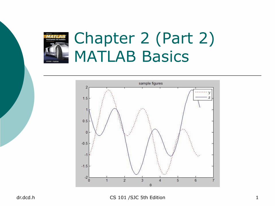
dr.dcd.h CS 101 /SJC 5th Edition 1 Chapter 2 (Part 2) MATLAB Basics
Transcript of Chapter 2 (Part 2) MATLAB Basics - NJIT SOShung/cs101/chap02-2.pdfChapter 2 (Part 2) MATLAB Basics ....
dr.dcd.h CS 101 /SJC 5th Edition 1
Chapter 2 (Part 2) MATLAB Basics
dr.dcd.h CS 101 /SJC 5th Edition 2
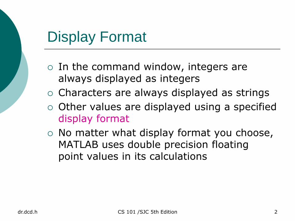
Display Format
In the command window, integers are always displayed as integers
Characters are always displayed as strings
Other values are displayed using a specified display format
No matter what display format you choose, MATLAB uses double precision floating point values in its calculations
dr.dcd.h CS 101 /SJC 5th Edition 3
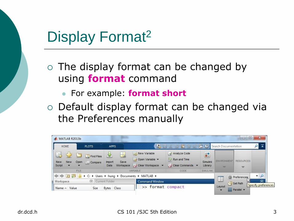
Display Format2
The display format can be changed by using format command
For example: format short
Default display format can be changed via the Preferences manually
dr.dcd.h CS 101 /SJC 5th Edition 4
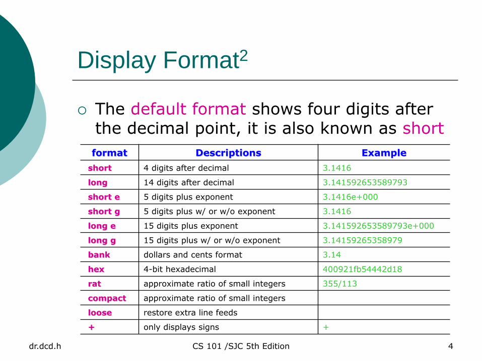
Display Format2
The default format shows four digits after the decimal point, it is also known as short
format Descriptions Example
short 4 digits after decimal 3.1416
long 14 digits after decimal 3.141592653589793
short e 5 digits plus exponent 3.1416e+000
short g 5 digits plus w/ or w/o exponent 3.1416
long e 15 digits plus exponent 3.141592653589793e+000
long g 15 digits plus w/ or w/o exponent 3.14159265358979
bank dollars and cents format 3.14
hex 4-bit hexadecimal 400921fb54442d18
rat approximate ratio of small integers 355/113
compact approximate ratio of small integers
loose restore extra line feeds
+ only displays signs +
dr.dcd.h CS 101 /SJC 5th Edition 5
The disp Function
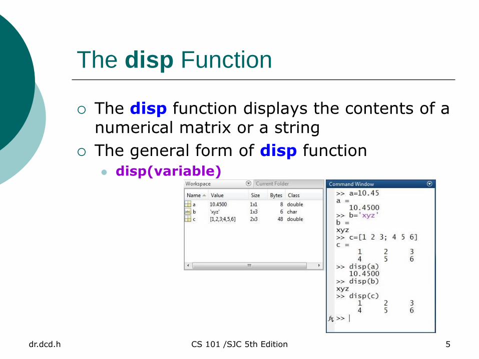
The disp function displays the contents of a numerical matrix or a string
The general form of disp function
disp(variable)
dr.dcd.h CS 101 /SJC 5th Edition 6
The disp Function2
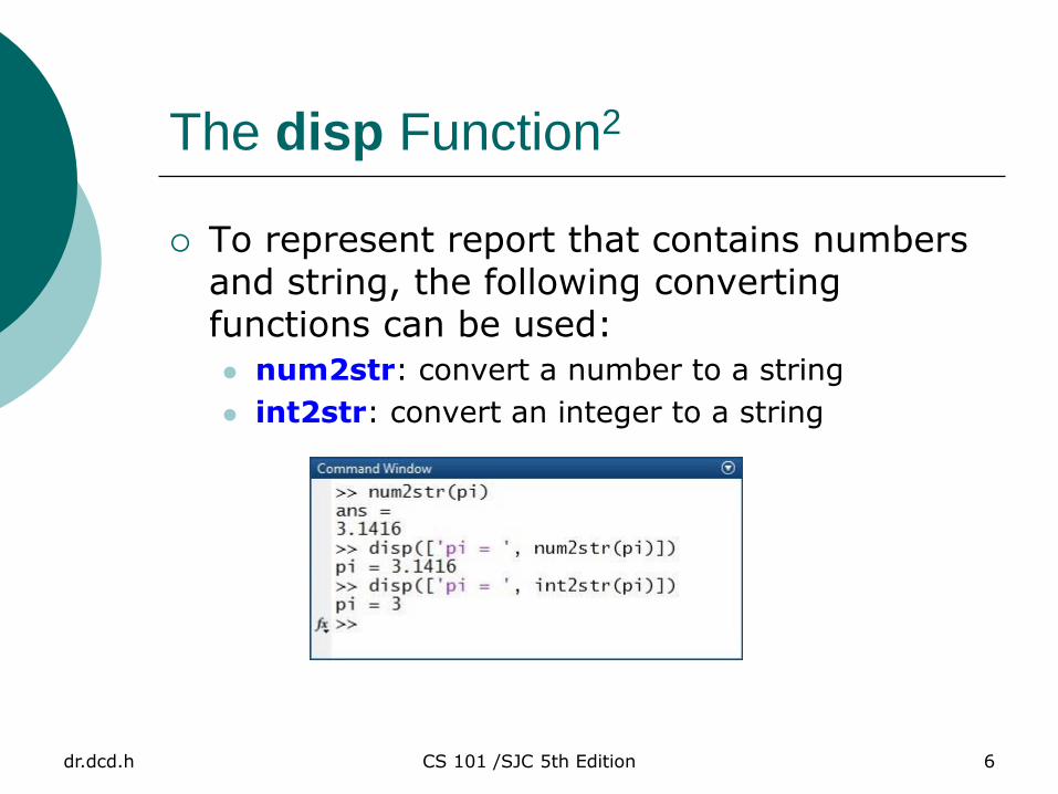
To represent report that contains numbers and string, the following converting functions can be used:
num2str: convert a number to a string
int2str: convert an integer to a string
dr.dcd.h CS 101 /SJC 5th Edition 7
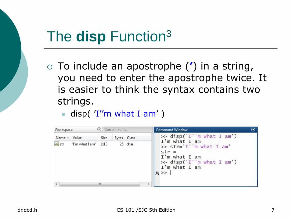
The disp Function3
To include an apostrophe (’) in a string, you need to enter the apostrophe twice. It is easier to think the syntax contains two strings.
disp( ’I’’m what I am’ )
dr.dcd.h CS 101 /SJC 5th Edition 8
Formatted Output: fprintf
fprintf function displays one or more values together with related text and provides control over the way values are displayed.
The general form of fprintf function
fprintf(format, data)
format is a string describing the way the data is to be printed
data is one or more scalars or arrays
dr.dcd.h CS 101 /SJC 5th Edition 9
Formatted Output: fprintf2
The general form of disp function
fprintf(format, data)
format is a string describing the way the data is to be printed
data is one or more scalars or arrays
The format is a string containing text plus special conversion characters describing the format of the data
dr.dcd.h CS 101 /SJC 5th Edition 10
Formatted Output: fprintf3
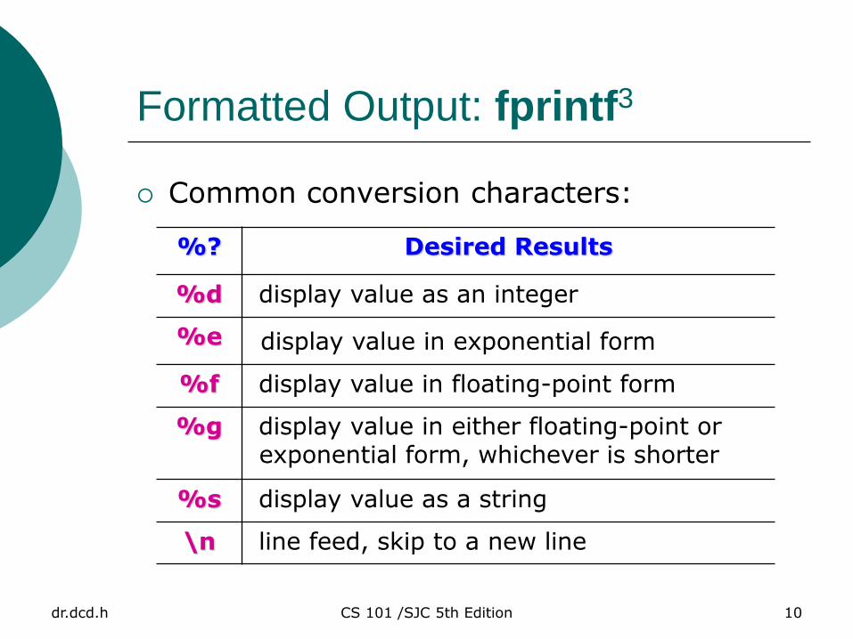
Common conversion characters:
%? Desired Results
%d display value as an integer
%e display value in exponential form
%f display value in floating-point form
%g display value in either floating-point or .exponential form, whichever is shorter
%s display value as a string
\n line feed, skip to a new line
dr.dcd.h CS 101 /SJC 5th Edition 11
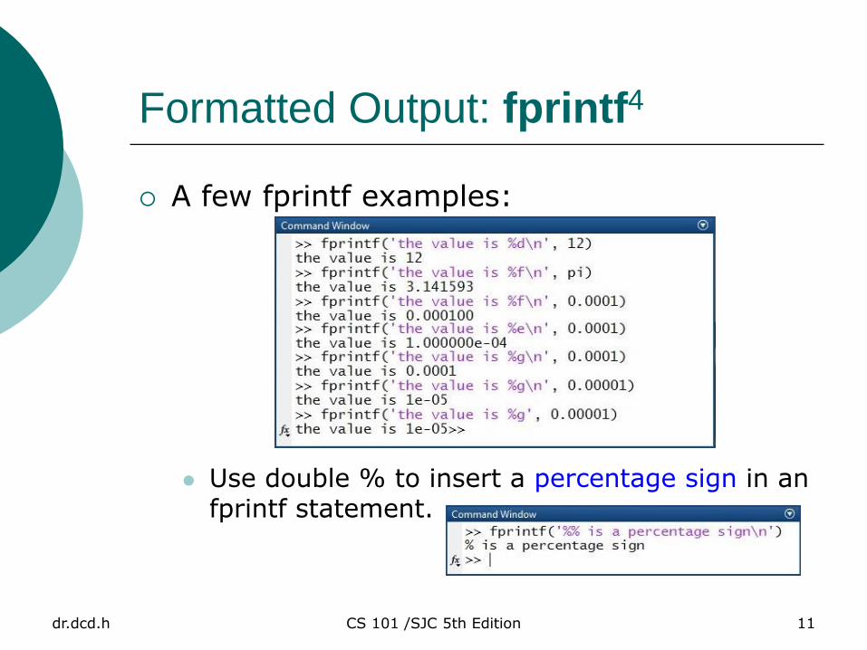
Formatted Output: fprintf4
A few fprintf examples:
Use double % to insert a percentage sign in an
fprintf statement.
dr.dcd.h CS 101 /SJC 5th Edition 12
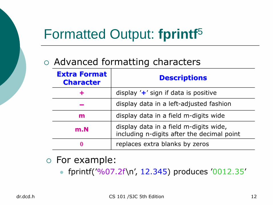
Formatted Output: fprintf5
Advanced formatting characters
Extra Format Character
Descriptions
+ display ’+’ sign if data is positive
– display data in a left-adjusted fashion
m display data in a field m-digits wide
m.N display data in a field m-digits wide, .including n-digits after the decimal point
0 replaces extra blanks by zeros
For example:
fprintf(’%07.2f\n’, 12.345) produces ’0012.35’
dr.dcd.h CS 101 /SJC 5th Edition 13
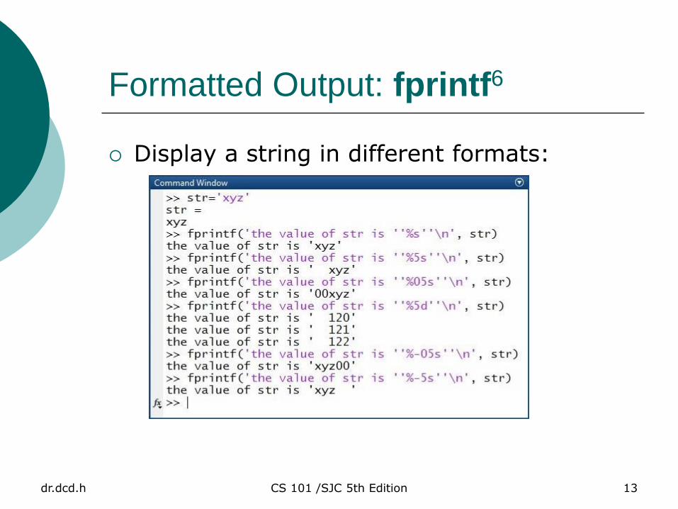
Formatted Output: fprintf6
Display a string in different formats:

dr.dcd.h CS 101 /SJC 5th Edition 14
Formatted Output: fprintf7
Display a number in different formats:
dr.dcd.h CS 101 /SJC 5th Edition 15
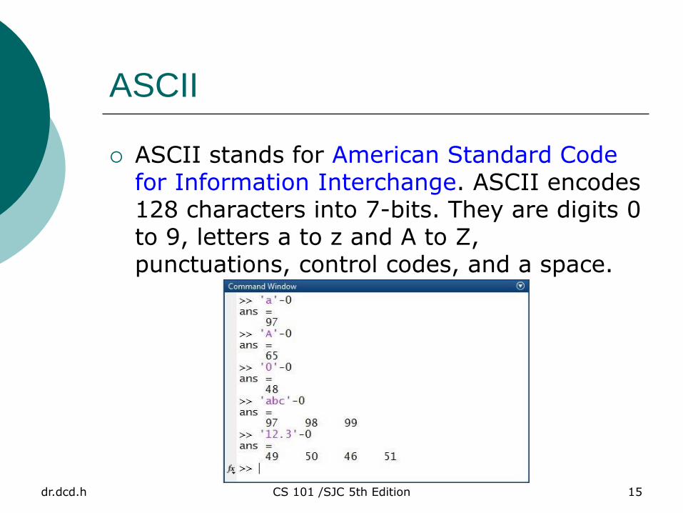
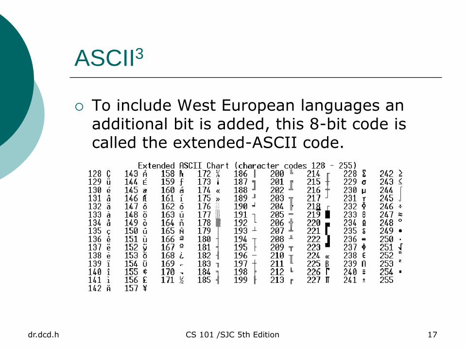
ASCII
ASCII stands for American Standard Code for Information Interchange. ASCII encodes 128 characters into 7-bits. They are digits 0 to 9, letters a to z and A to Z, punctuations, control codes, and a space.

dr.dcd.h CS 101 /SJC 5th Edition 16
ASCII2
The ASCII chart:
dr.dcd.h CS 101 /SJC 5th Edition 17
ASCII3
To include West European languages an additional bit is added, this 8-bit code is called the extended-ASCII code.

dr.dcd.h CS 101 /SJC 5th Edition 18
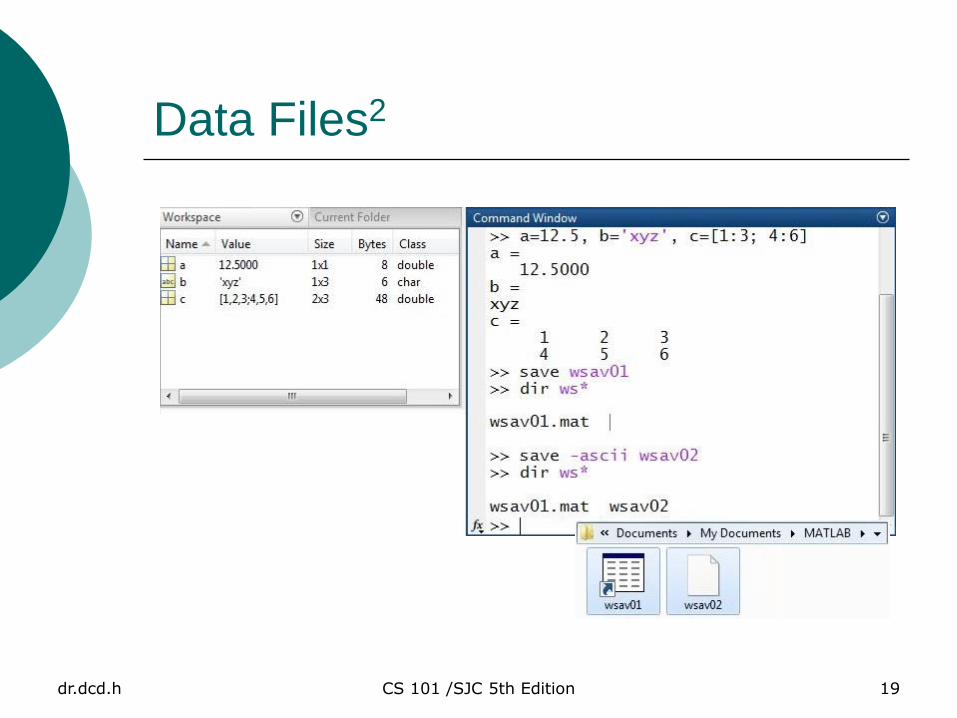
Data Files
The save command saves data from the current workspace into a disk file.
The general form of save function
save <–ascii> filename <var_list>
By default, the filename will be given the extension mat.
If no variables are specified, all variables in the workspace will be saved.
If option –ascii is used, the data will be saved in an ASCII file with the exponential form.
dr.dcd.h CS 101 /SJC 5th Edition 19
Data Files2
dr.dcd.h CS 101 /SJC 5th Edition 20
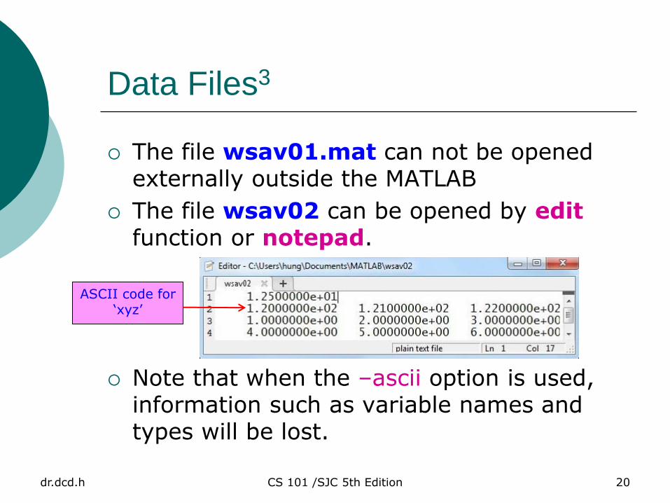
Data Files3
The file wsav01.mat can not be opened externally outside the MATLAB
The file wsav02 can be opened by edit function or notepad.
Note that when the –ascii option is used, information such as variable names and types will be lost.
ASCII code for ‘xyz’
dr.dcd.h CS 101 /SJC 5th Edition 21
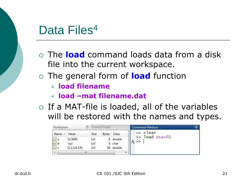
Data Files4
The load command loads data from a disk file into the current workspace.
The general form of load function
load filename
load –mat filename.dat
If a MAT-file is loaded, all of the variables will be restored with the names and types.
dr.dcd.h CS 101 /SJC 5th Edition 22
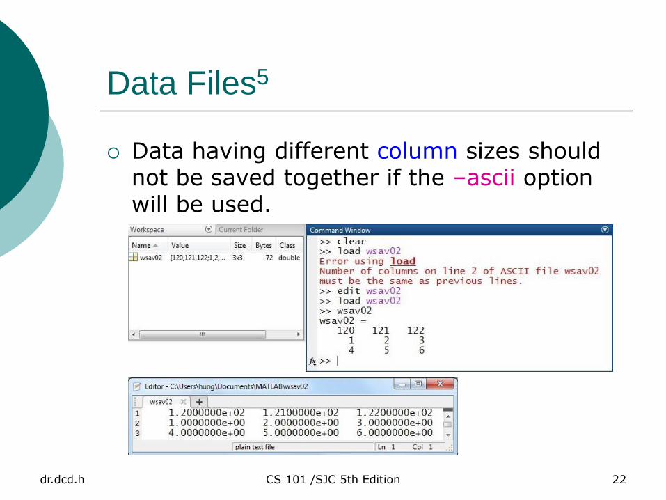
Data Files5
Data having different column sizes should not be saved together if the –ascii option will be used.
dr.dcd.h CS 101 /SJC 5th Edition 23
Data Files6
The contents of an ASCII-file will be converted into an array having the same name as the file (w/o the extension).
Data having different column sizes should not be saved together if the –ascii option will be used.

dr.dcd.h CS 101 /SJC 5th Edition 24
Scalar Arithmetic Operations
Arithmetic Operation
Algebraic Form MATLAB Form
Addition a + b a + b
Subtraction a – b a – b
Multiplication a x b a * b
Division a b
a / b or b \ a
Exponentiation ab a ^ b
____
Note:
b\a is called the left division.
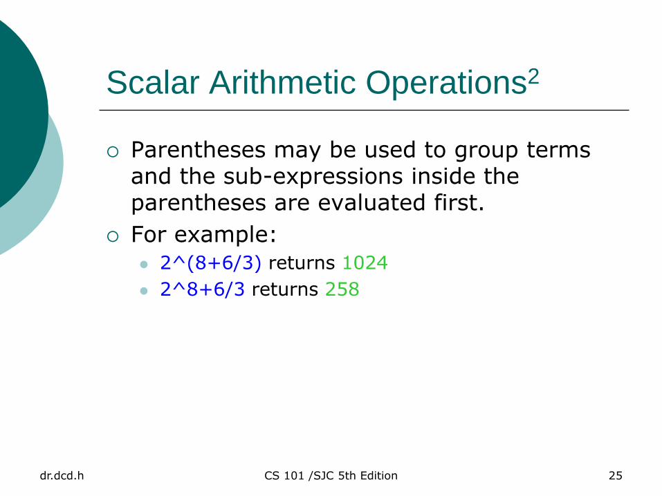
Parentheses may be used to group terms and the sub-expressions inside the parentheses are evaluated first.
dr.dcd.h CS 101 /SJC 5th Edition 25
Scalar Arithmetic Operations2
Parentheses may be used to group terms and the sub-expressions inside the parentheses are evaluated first.
For example:
2^(8+6/3) returns 1024
2^8+6/3 returns 258
dr.dcd.h CS 101 /SJC 5th Edition 26
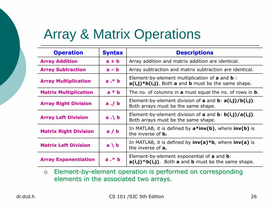
Array & Matrix Operations Operation Syntax Descriptions
Array Addition a + b Array addition and matrix addition are identical.
Array Subtraction a – b Array subtraction and matrix subtraction are identical.
Array Multiplication a .* b Element-by-element multiplication of a and b : a(i,j)*b(i,j). Both a and b must be the same shape.
Matrix Multiplication a * b The no. of columns in a must equal the no. of rows in b.
Array Right Division a ./ b Element-by-element division of a and b: a(i,j)/b(i,j). Both arrays must be the same shape.
Array Left Division a .\ b Element-by-element division of a and b: b(i,j)/a(i,j). Both arrays must be the same shape.
Matrix Right Division a / b In MATLAB, it is defined by a*inv(b), where inv(b) is the inverse of b.
Matrix Left Division a \ b In MATLAB, it is defined by inv(a)*b, where inv(a) is the inverse of a.
Array Exponentiation a .^ b Element-by-element exponential of a and b: a(i,j)^b(i,j). Both a and b must be the same shape.
Element-by-element operation is performed on corresponding elements in the associated two arrays.

dr.dcd.h CS 101 /SJC 5th Edition 27
Array & Matrix Operations2
Array operation between two arrays:
Array multiplication:
Matrix multiplication:
dr.dcd.h CS 101 /SJC 5th Edition 28
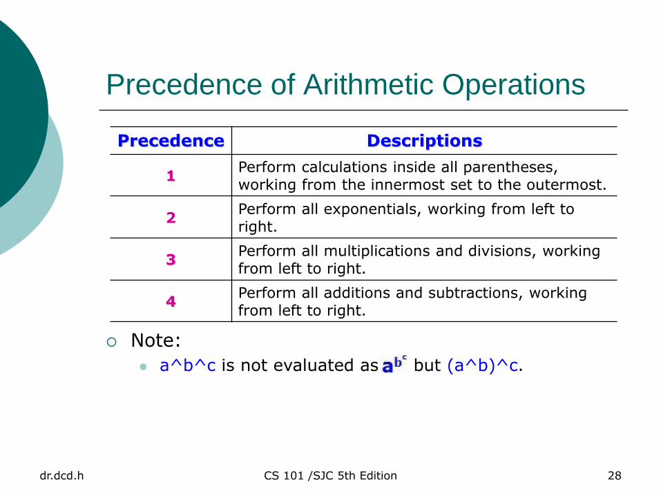
Precedence of Arithmetic Operations
Precedence Descriptions
1 Perform calculations inside all parentheses, working from the innermost set to the outermost.
2 Perform all exponentials, working from left to right.
3 Perform all multiplications and divisions, working from left to right.
4 Perform all additions and subtractions, working from left to right.
Note:
a^b^c is not evaluated as but (a^b)^c.
dr.dcd.h CS 101 /SJC 5th Edition 29
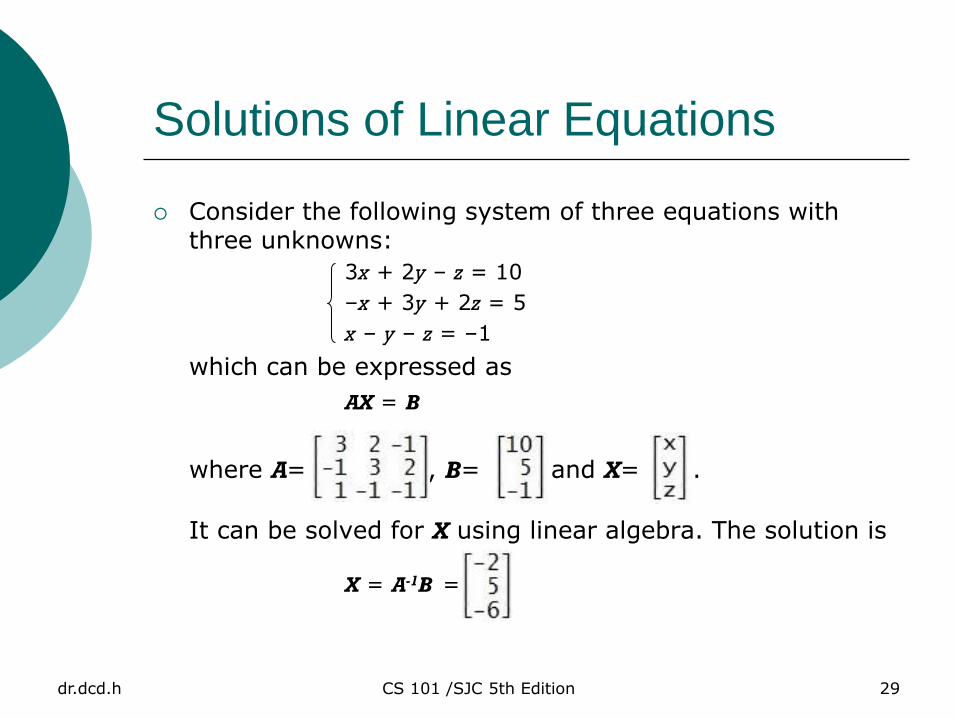
Solutions of Linear Equations
Consider the following system of three equations with three unknowns:
3x + 2y – z = 10
–x + 3y + 2z = 5
x – y – z = –1
which can be expressed as
AX = B
where A= , B= and X= .
It can be solved for X using linear algebra. The solution is
X = A-1B =

dr.dcd.h CS 101 /SJC 5th Edition 30
Homework Assignment #4
Quiz 2.3
Page 51: 2, 3
Quiz 2.4
Page 58: 1, 2
This assignment is due by next week.
Late submission will be penalized.
dr.dcd.h CS 101 /SJC 5th Edition 31
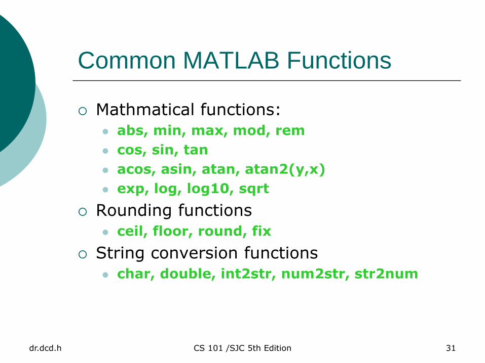
Common MATLAB Functions
Mathmatical functions:
abs, min, max, mod, rem
cos, sin, tan
acos, asin, atan, atan2(y,x)
exp, log, log10, sqrt
Rounding functions
ceil, floor, round, fix
String conversion functions
char, double, int2str, num2str, str2num
dr.dcd.h CS 101 /SJC 5th Edition 32
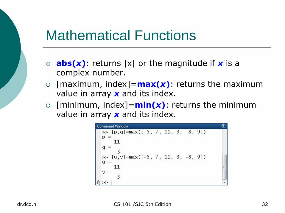
Mathematical Functions
abs(x): returns |x| or the magnitude if x is a complex number.
[maximum, index]=max(x): returns the maximum value in array x and its index.
[minimum, index]=min(x): returns the minimum value in array x and its index.
dr.dcd.h CS 101 /SJC 5th Edition 33
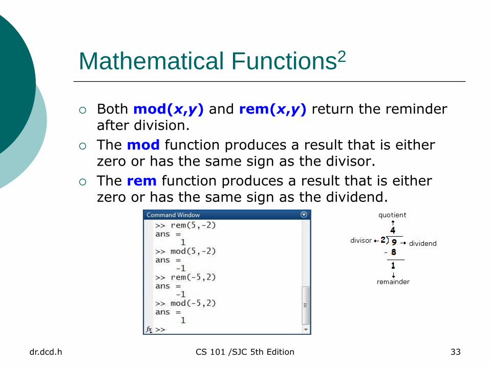
Mathematical Functions2
Both mod(x,y) and rem(x,y) return the reminder after division.
The mod function produces a result that is either zero or has the same sign as the divisor.
The rem function produces a result that is either zero or has the same sign as the dividend.
dr.dcd.h CS 101 /SJC 5th Edition 34
Mathematical Functions3
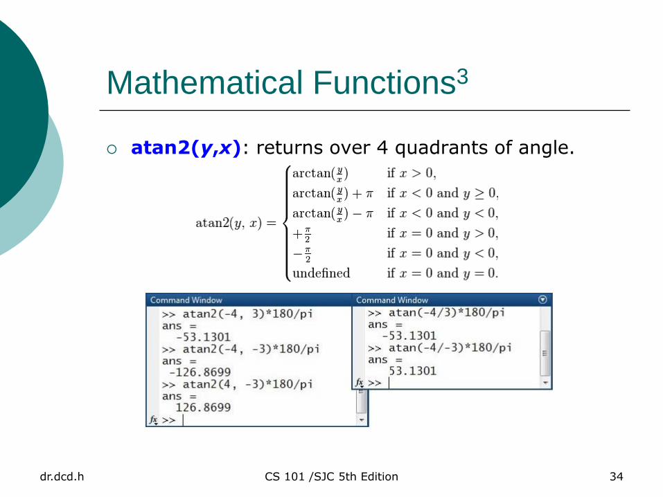
atan2(y,x): returns over 4 quadrants of angle.
dr.dcd.h CS 101 /SJC 5th Edition 35
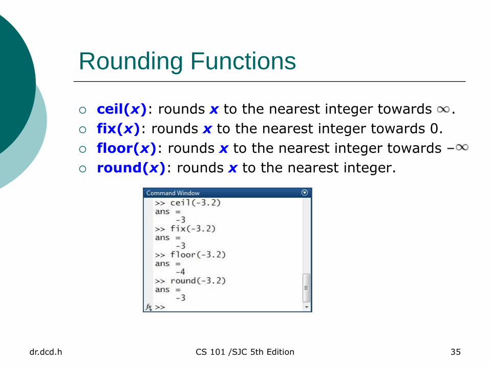
Rounding Functions
ceil(x): rounds x to the nearest integer towards .
fix(x): rounds x to the nearest integer towards 0.
floor(x): rounds x to the nearest integer towards –
round(x): rounds x to the nearest integer.
dr.dcd.h CS 101 /SJC 5th Edition 36
String Conversion Functions
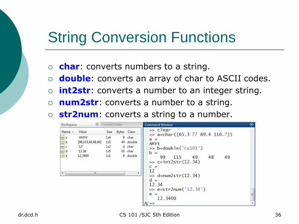
char: converts numbers to a string.
double: converts an array of char to ASCII codes.
int2str: converts a number to an integer string.
num2str: converts a number to a string.
str2num: converts a string to a number.
dr.dcd.h CS 101 /SJC 5th Edition 37
Two-Dimensional Plots
The general form of plot function
plot(x, y)
y is a 1-1 function of x
When plot is execute, a figure window opens.
Title and axis labels can be added by
title(str)
xlabel(str)
ylabel(str)
Grid lines can be enabled/disable by
grid on/off

dr.dcd.h CS 101 /SJC 5th Edition 38
Two-Dimensional Plots2
dr.dcd.h CS 101 /SJC 5th Edition 39
Save Plots
The print command can be used to save a plot as an image from a M-script
print <option> filename
Valid options
–deps: monochrome encapsulated postscript ___ __ image
–depsc: color encapsulated postscript image
–djpeg: JPEG image
–dpng: portable network graphic image
–dtiff: compressed TIFF image
dr.dcd.h CS 101 /SJC 5th Edition 40
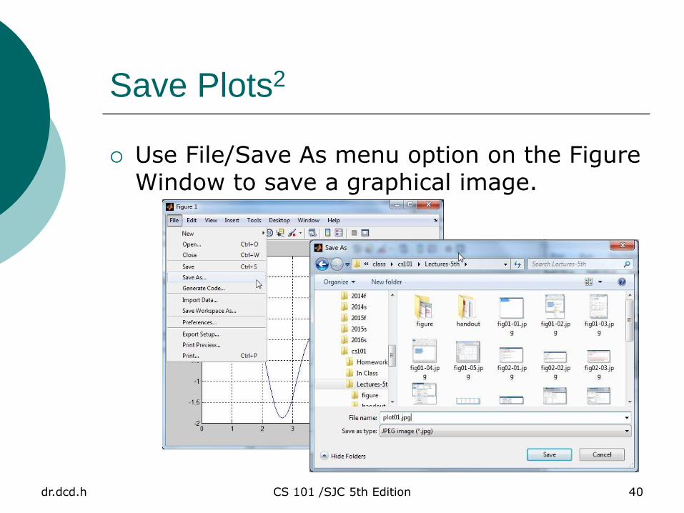
Save Plots2
Use File/Save As menu option on the Figure Window to save a graphical image.
dr.dcd.h CS 101 /SJC 5th Edition 41
Multiple Plots
1st method: plot two functions y1=f(x1) and y2=g(x2) at once
plot(x1, y1, x2, y2, …)
x1 and x2 can be defined over different ranges
For example:
f(x) = sin(2x)
The first derivation of f(x) = 2 cos(2x)
To plot them side-by-side for comparison
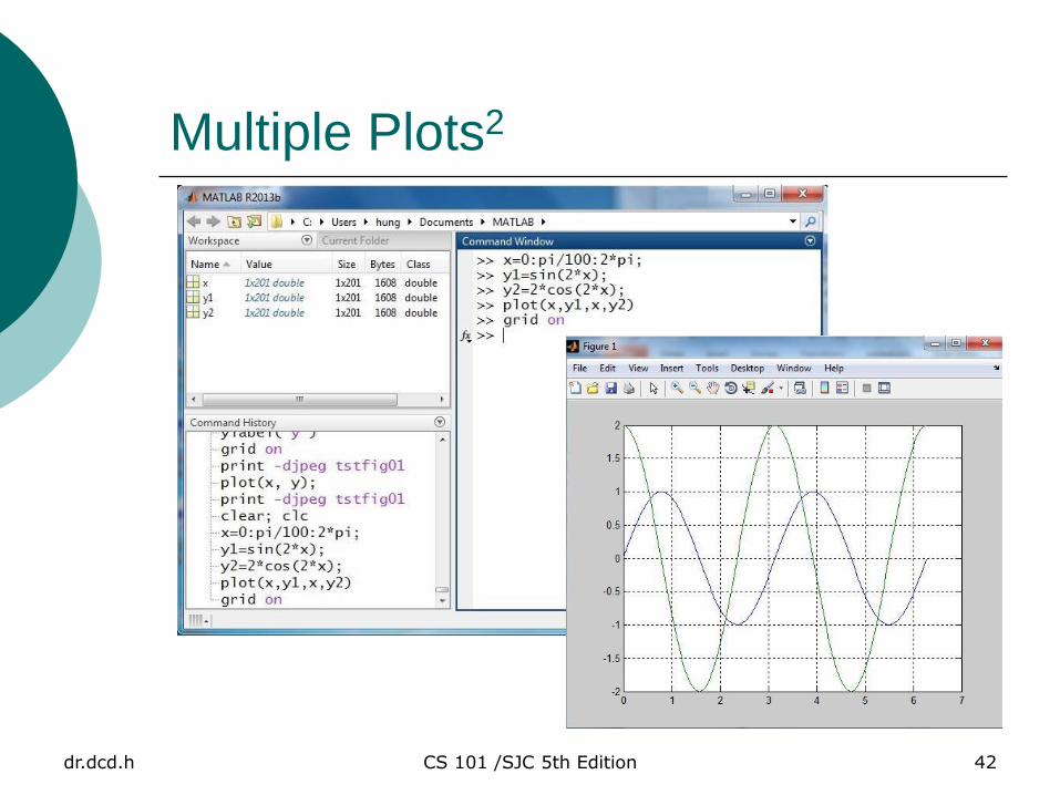
dr.dcd.h CS 101 /SJC 5th Edition 42
Multiple Plots2
dr.dcd.h CS 101 /SJC 5th Edition 43
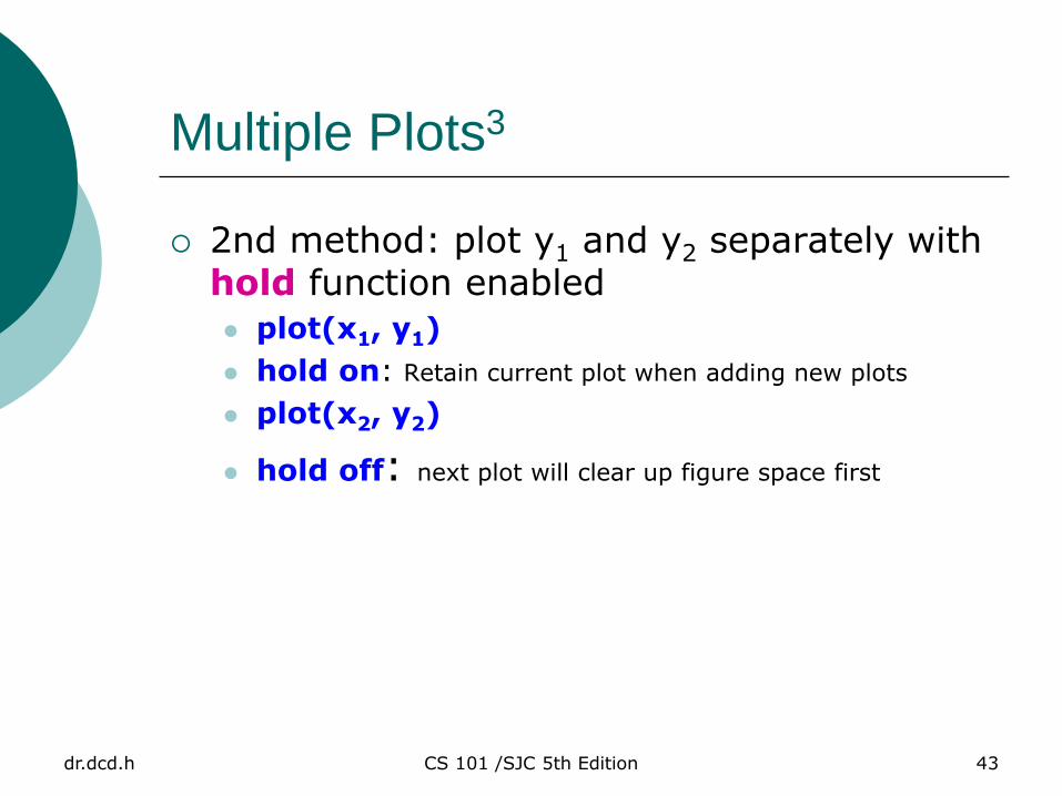
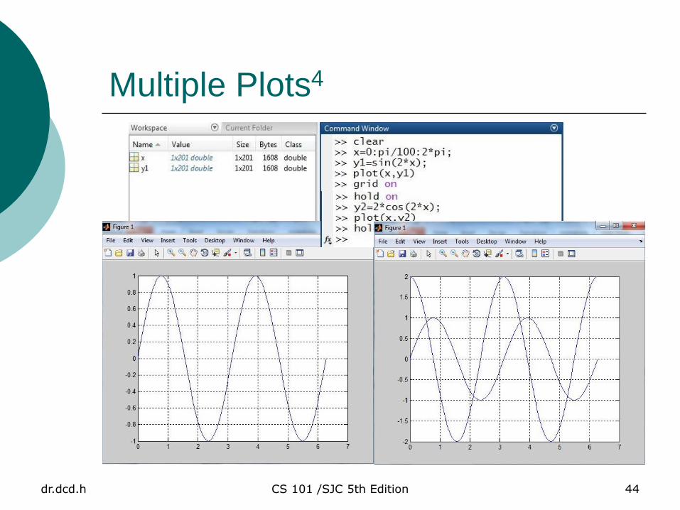
Multiple Plots3
2nd method: plot y1 and y2 separately with hold function enabled
plot(x1, y1)
hold on: Retain current plot when adding new plots
plot(x2, y2)
hold off: next plot will clear up figure space first
dr.dcd.h CS 101 /SJC 5th Edition 44
Multiple Plots4
dr.dcd.h CS 101 /SJC 5th Edition 45
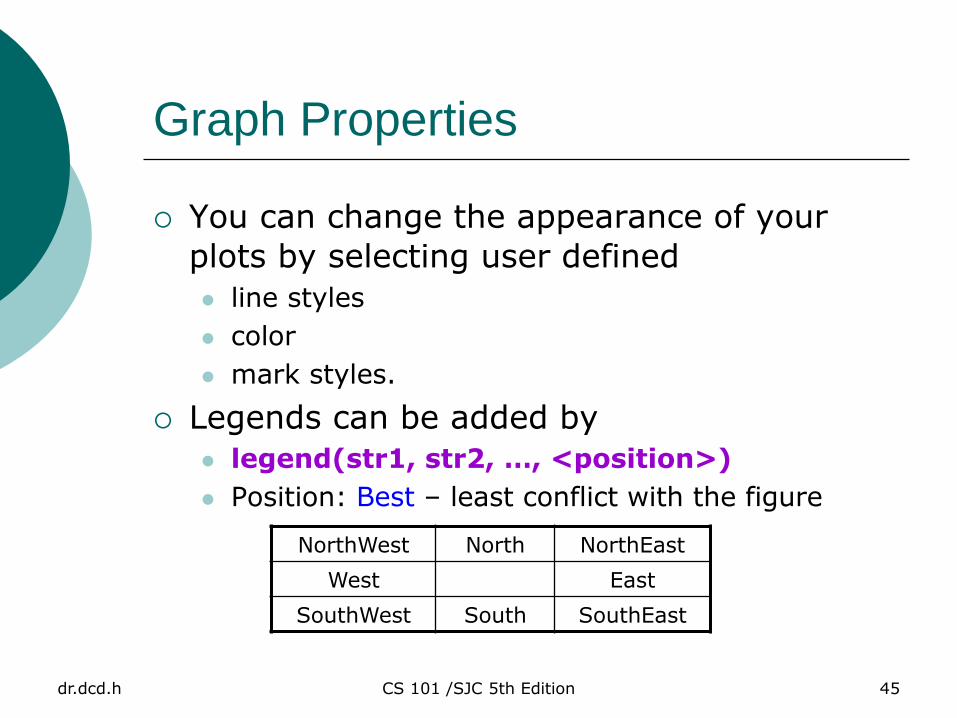
Graph Properties
You can change the appearance of your
plots by selecting user defined line styles
color
mark styles.
Legends can be added by
legend(str1, str2, …, <position>)
Position: Best – least conflict with the figure
NorthWest North NorthEast
West East
SouthWest South SouthEast
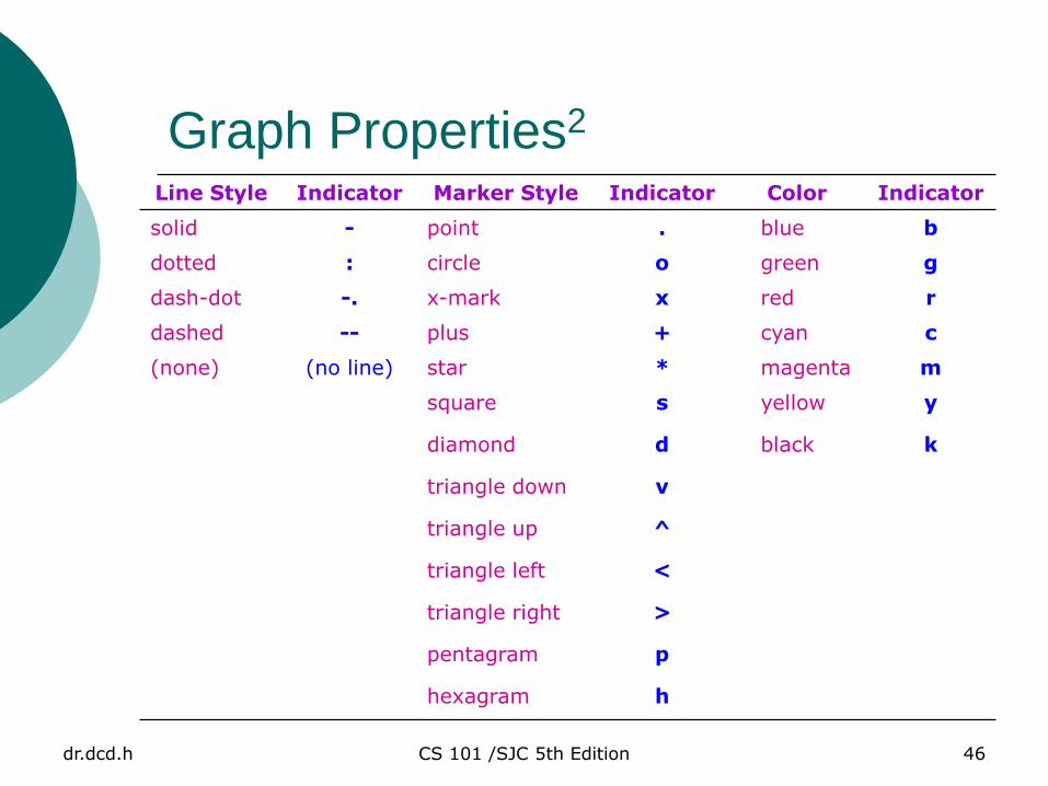
dr.dcd.h CS 101 /SJC 5th Edition 46
Graph Properties2
Line Style Indicator Marker Style Indicator Color Indicator
solid - point . blue b
dotted : circle o green g
dash-dot -. x-mark x red r
dashed -- plus + cyan c
(none) (no line) star * magenta m
square s yellow y
diamond d black k
triangle down v
triangle up ^
triangle left <
triangle right >
pentagram p
hexagram h

dr.dcd.h CS 101 /SJC 5th Edition 47
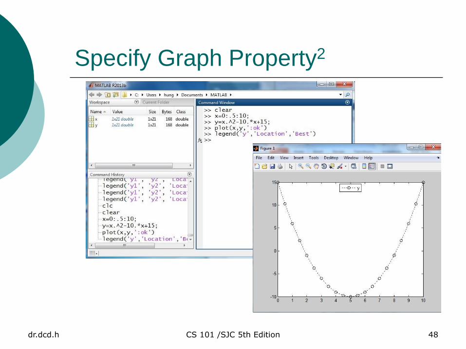
Specify Graph Property
plot(x, y, opstr)
Opstr combining line style, marker style, and color
For example: ’:ok’ indicates dotted line ’:’, circle marker ’o’, and black color ’k’.
legend(str_list, ’Location’, ’Best’)
Best – least conflict with the figure
All locations can be outside plot, eg. ’BestOutside’
dr.dcd.h CS 101 /SJC 5th Edition 48
Specify Graph Property2
dr.dcd.h CS 101 /SJC 5th Edition 49
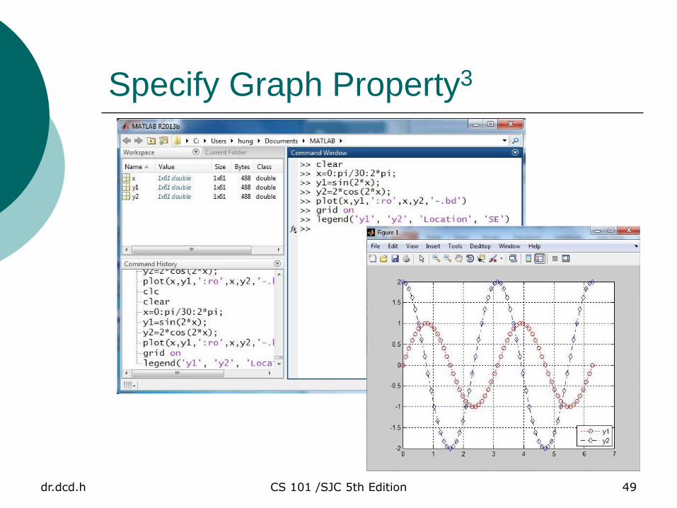
Specify Graph Property3
dr.dcd.h CS 101 /SJC 5th Edition 50
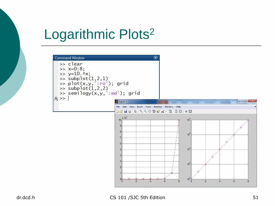
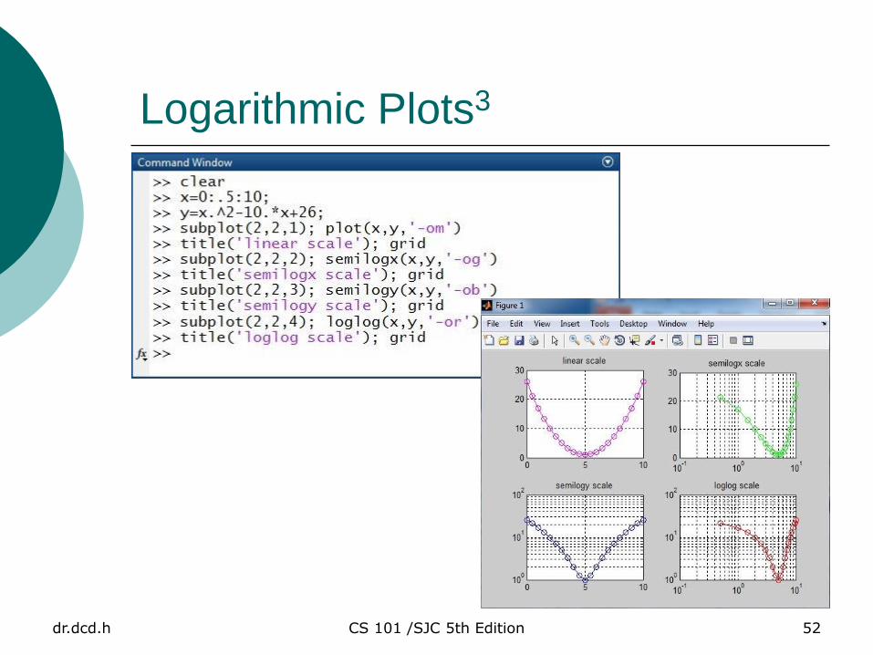
Logarithmic Plots
A logarithmic scale (base 10) is useful if a variable ranges over many orders of magnitude, or data varies exponentially.
semilogy – uses a log10 scale on the y axis
semilogx – uses a log10 scale on the x axis
loglog – uses a log10 scale on both axes
dr.dcd.h CS 101 /SJC 5th Edition 51
Logarithmic Plots2
dr.dcd.h CS 101 /SJC 5th Edition 52
Logarithmic Plots3
dr.dcd.h CS 101 /SJC 5th Edition 53
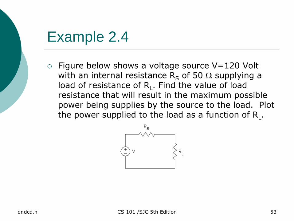
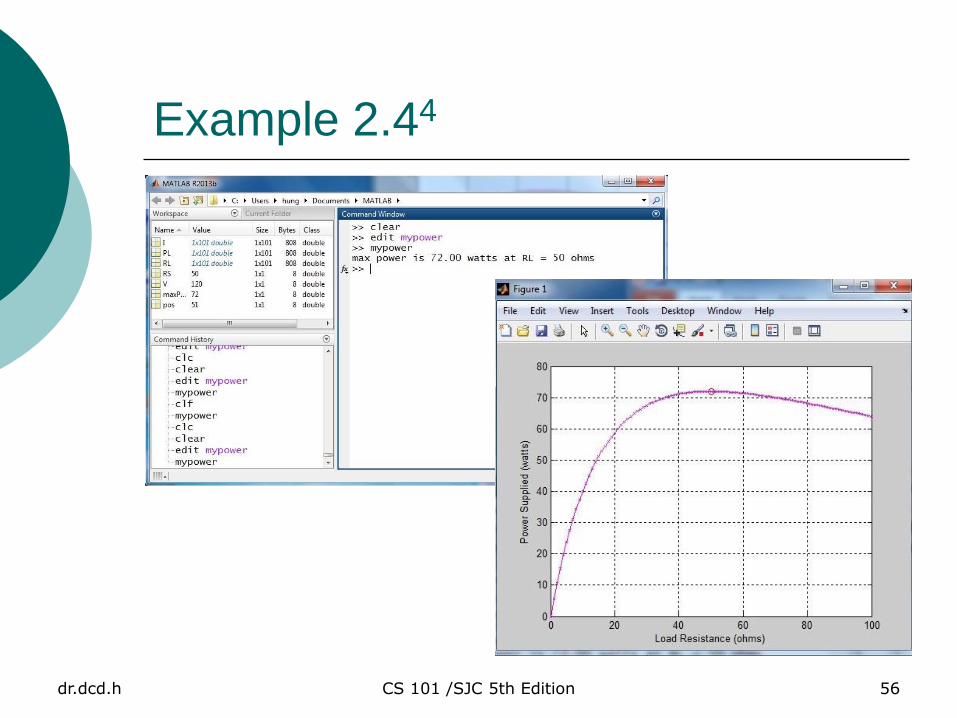
Example 2.4
Figure below shows a voltage source V=120 Volt with an internal resistance RS of 50 W supplying a load of resistance of RL. Find the value of load resistance that will result in the maximum possible power being supplies by the source to the load. Plot the power supplied to the load as a function of RL.

dr.dcd.h CS 101 /SJC 5th Edition 54
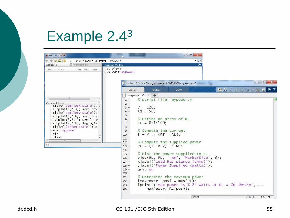
Example 2.42
The power supplied to the load RL is given by
PL = I2 RL
where I is the current supplied to the load, it can be obtained by Ohm’s law
V
RS+RL
Procedures to perform the work:
Define an array of possible values for RL
Compute the current for each value of RL
Compute the supplied power for each value of RL
Plot the power supplied to the load for each value of RL
Determine the maximum power
_______
dr.dcd.h CS 101 /SJC 5th Edition 55
Example 2.43
dr.dcd.h CS 101 /SJC 5th Edition 56
Example 2.44

dr.dcd.h CS 101 /SJC 5th Edition 57
Homework Assignment #5
2.15 Exercises
Page 83: 2.1 - 2.8
This assignment is due by next week.
Late submission will be penalized.